
Remote Sensing Observation of Particulate Organic Carbon in the Pearl River Estuary

Abstract
:
1. Introduction
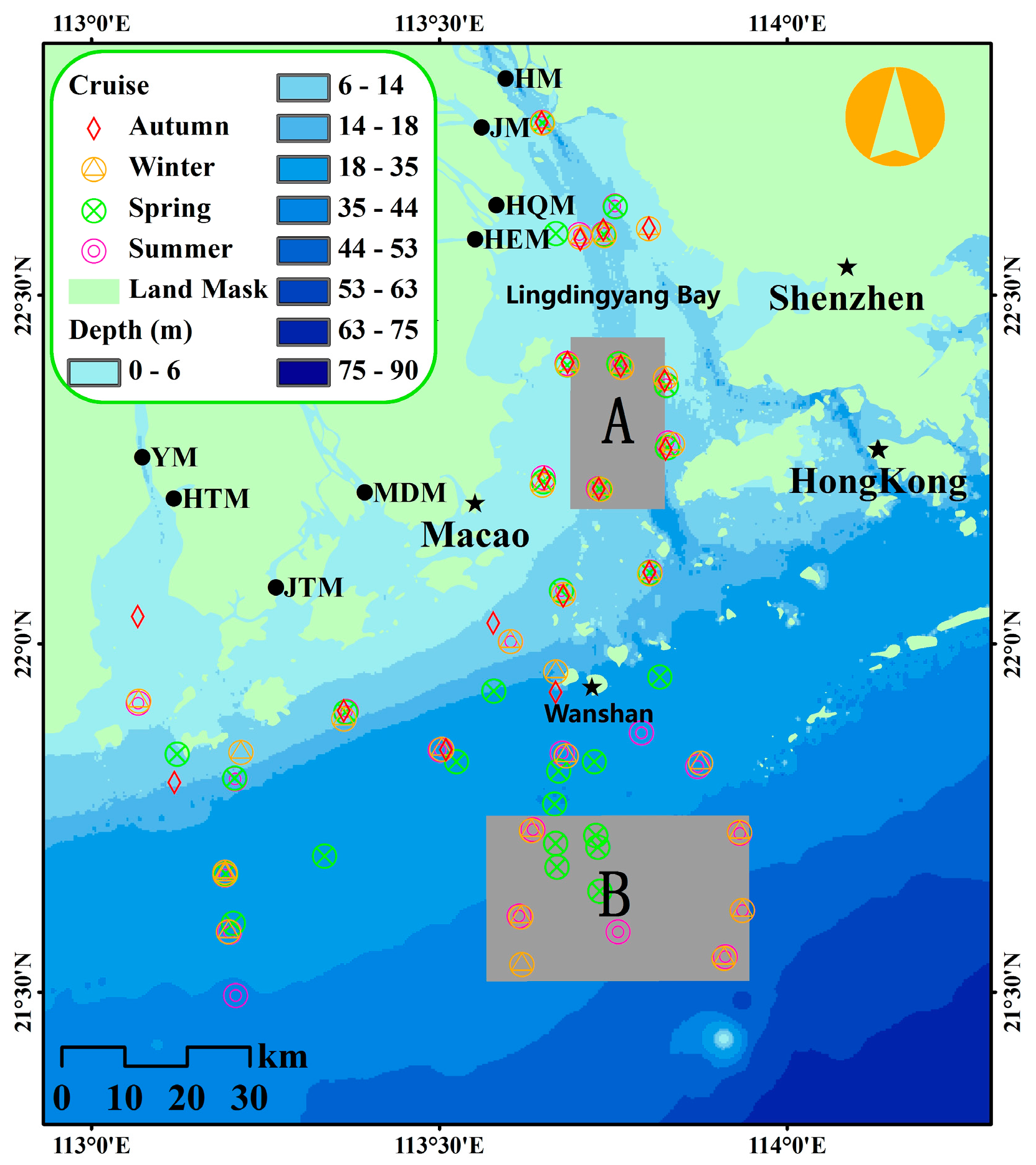
2. Study Area
3. Materials
3.1. Field Sampling and Laboratory Analyses
3.2. Measurement of Remote Sensing Reflectance

3.3. Satellite Ocean Color Data
4. Algorithm Development
5. Results
5.1. Application of the Developed Algorithm
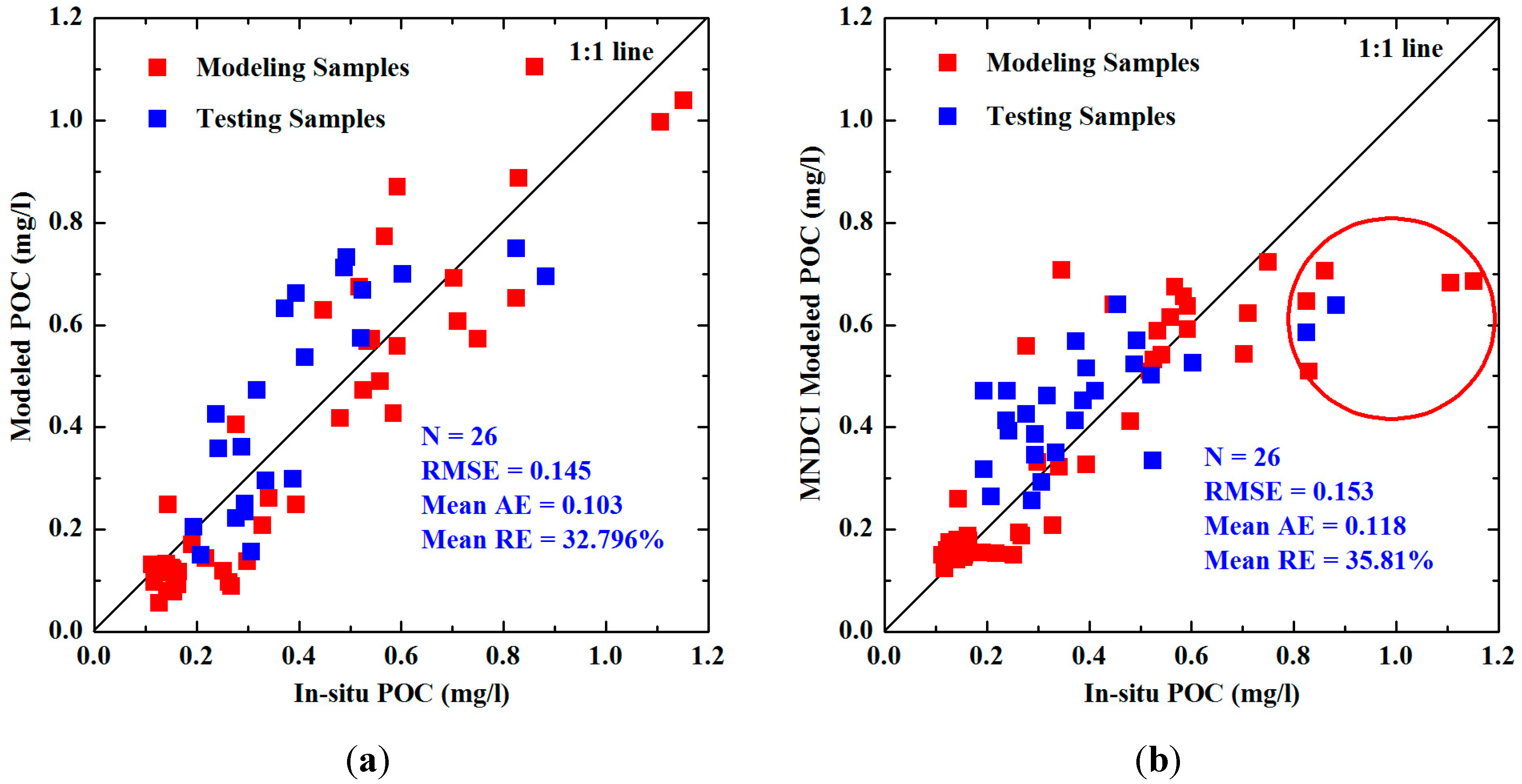
5.1.1. Application to in Situ Data
5.1.2. Application to MODIS/AQUA Data

| No. | Sampling Day | Sampling Time | In Situ POC (mg/L) | Modeled POC (mg/L) | AE (mg/L) | RE (%) |
|---|---|---|---|---|---|---|
| 1 | 27/2/2014 | 14:55 | 0.121 | 0.120 | 0.002 | 1.653 |
| 2 | 27/2/2014 | 14:04 | 0.150 | 0.117 | 0.033 | 22 |
| 3 | 27/2/2014 | 10:06 | 0.126 | 0.067 | 0.059 | 46.825 |
| 4 | 27/2/2014 | 11:15 | 0.113 | 0.077 | 0.036 | 31.858 |
| 5 | 24/8/2014 | 14:11 | 0.861 | 0.860 | 0.001 | 0.116 |
| 6 | 24/8/2014 | 9:24 | 1.402 | 0.926 | 0.476 | 33.952 |
| 7 | 24/8/2014 | 15:14 | 0.446 | 0.475 | 0.028 | 6.278 |
| 8 | 30/8/2014 | 12:00 | 0.829 | 0.755 | 0.074 | 8.926 |
| 9 | 30/8/2014 | 9:26 | 0.711 | 0.895 | 0.185 | 26.02 |
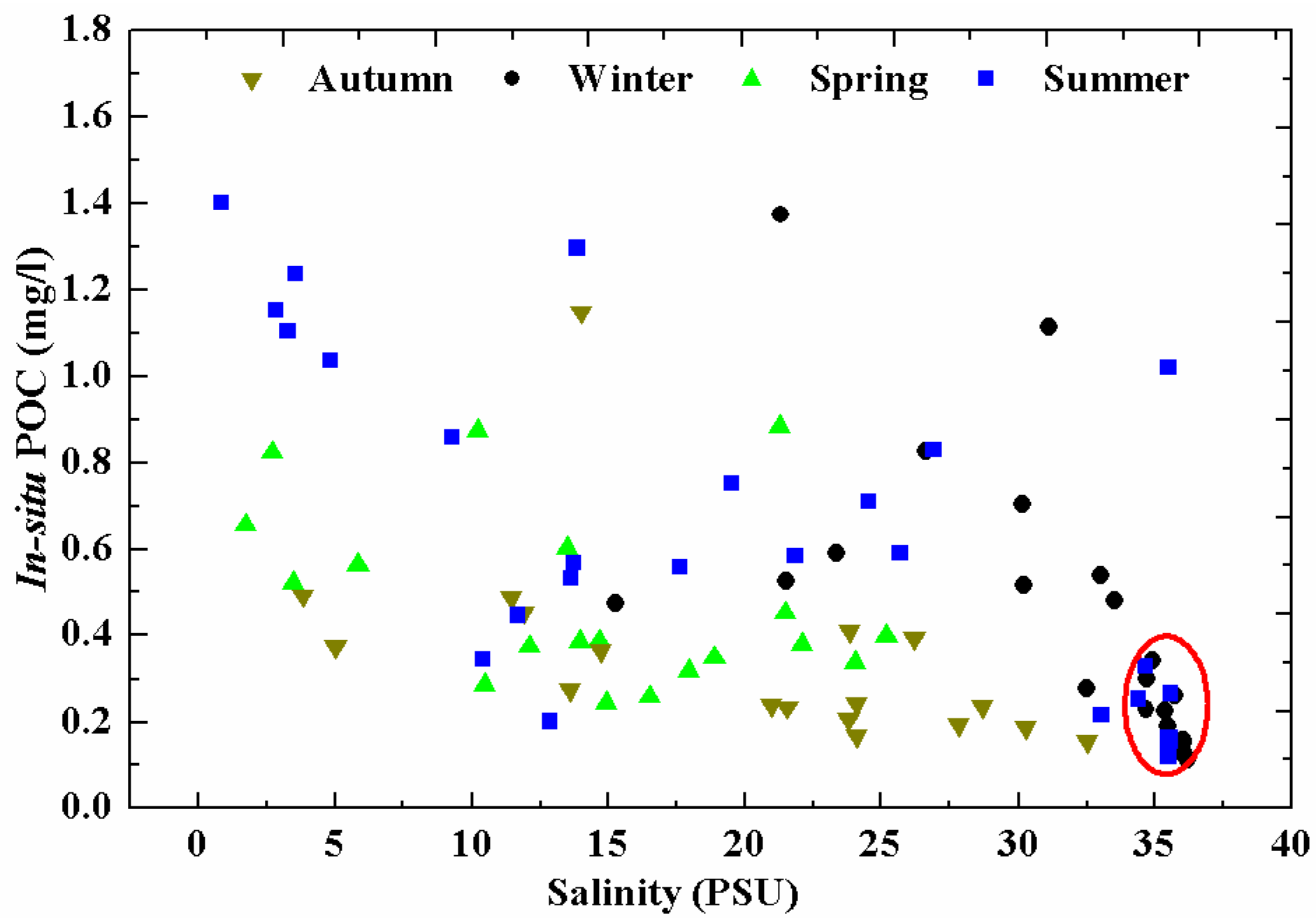
5.2. Particulate Organic Carbon (POC) Distribution from in situ Data
| Cruise | Samples | Min | Max | Median | Mean |
|---|---|---|---|---|---|
| Autumn | 18 | 0.156 | 1.150 | 0.260 | 0.348 |
| Winter | 27 | 0.113 | 1.374 | 0.277 | 0.393 |
| Spring | 29 | 0.194 | 0.883 | 0.372 | 0.420 |
| Summer | 29 | 0.118 | 1.402 | 0.557 | 0.592 |
| All | 103 | 0.113 | 1.402 | 0.349 | 0.449 |
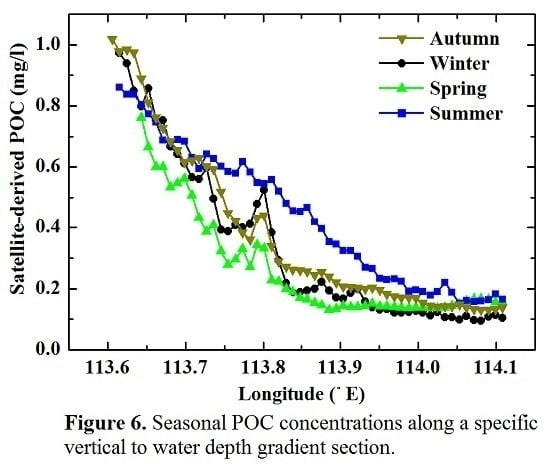
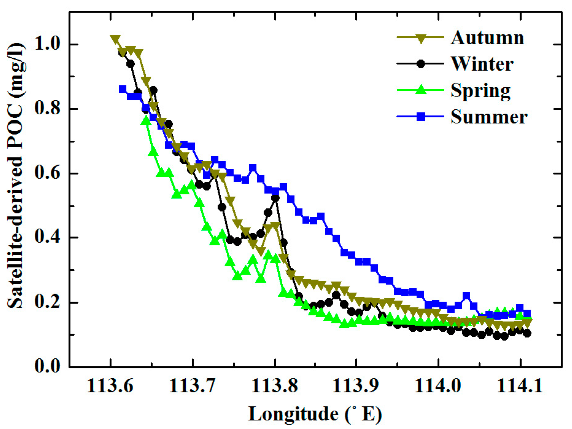
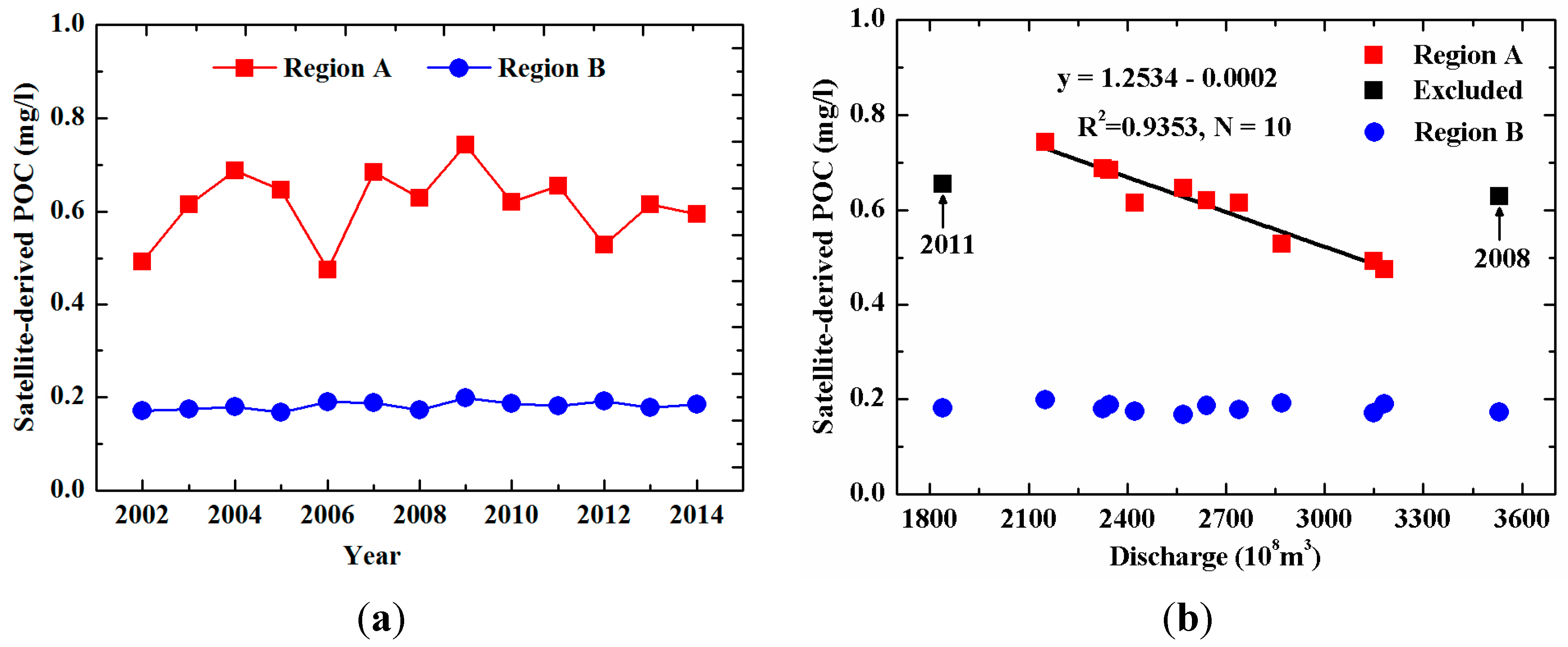
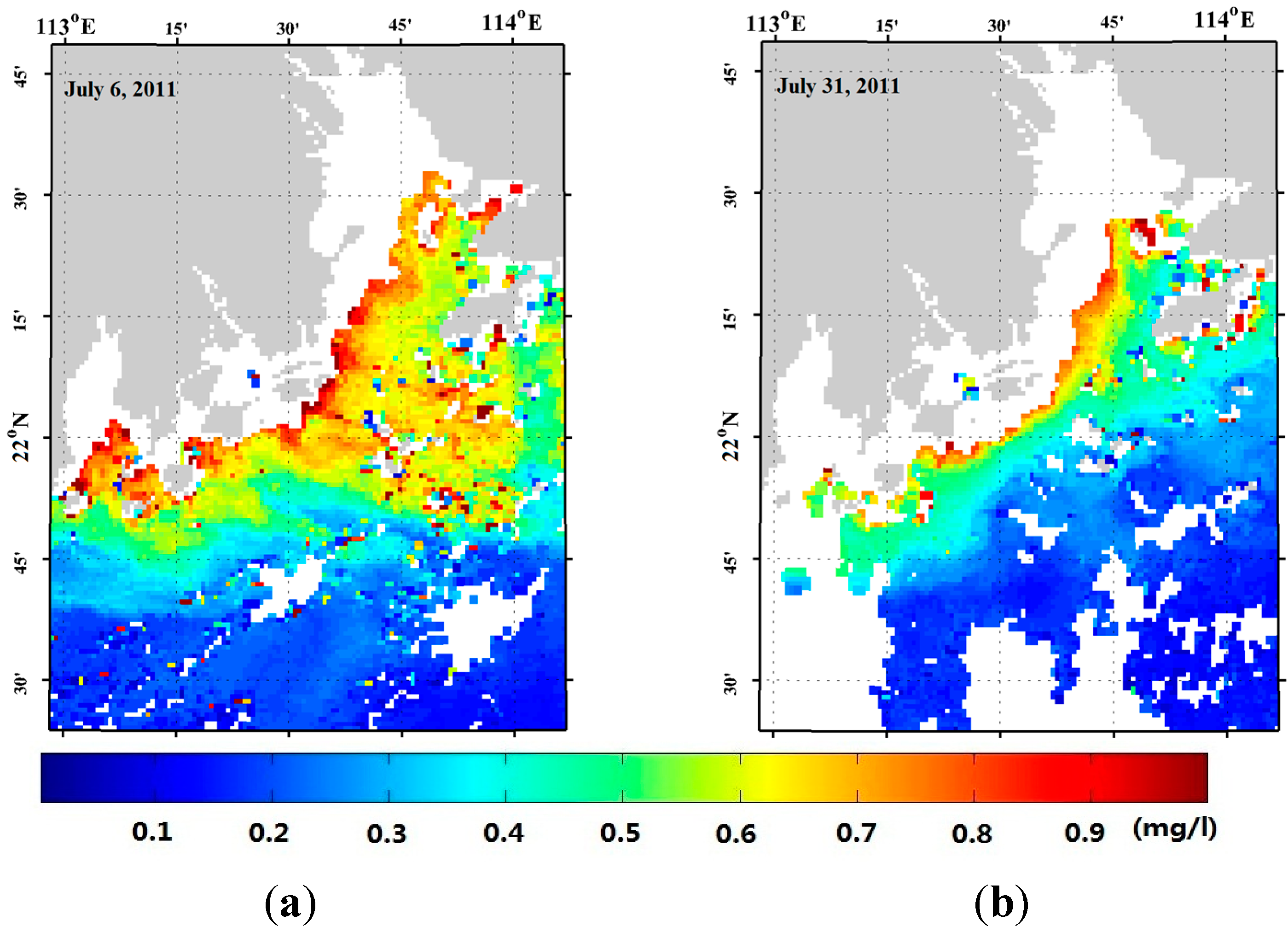
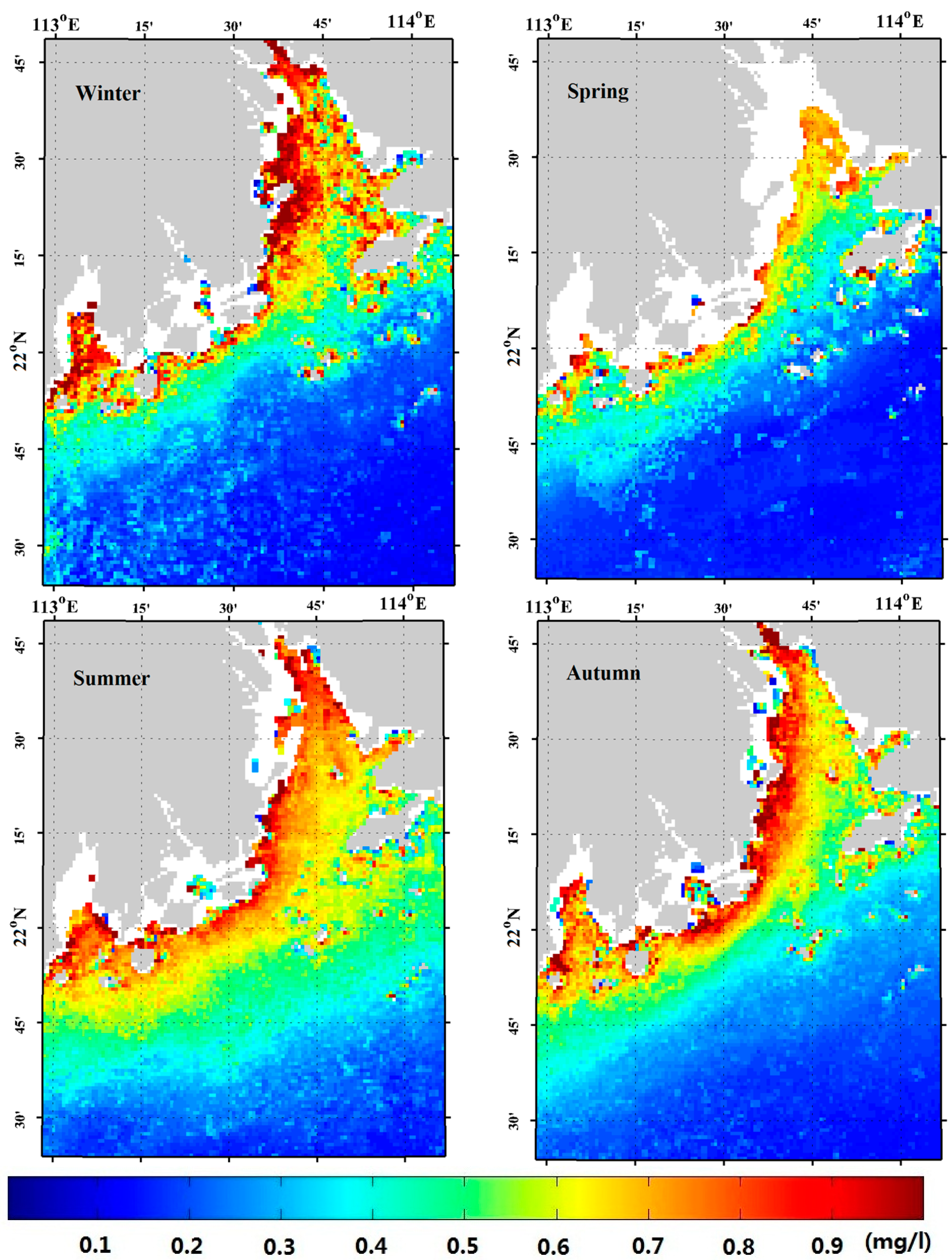
5.3. Temporal and Spatial Variations from Satellite-Derived POC


6. Discussions
6.1. Sources of POC in the Pearl River Estuary


| Season | Phytoplankton POC (%) | |
|---|---|---|
| In-shore Waters | Off-shore Waters | |
| Autumn | 33.26 | 45.3 |
| Winter | 62.5 | 40.59 |
| Spring | 29.16 | 65.32 |
6.2. Impact Factors on POC Distribution in the PRE

7. Conclusions
Acknowledgments
Author Contributions
Conflicts of Interest
References
- Zhu, Z.Y.; Zhang, J.; Wu, Y.; Lin, J. Bulk particulate organic carbon in the East China Sea: Tidal influence and bottom transport. Prog. Oceanogr. 2006, 69, 37–60. [Google Scholar] [CrossRef]
- Stramska, M. Particulate organic carbon in the global ocean derived from SeaWiFS ocean color. Deep Sea Res. I 2009, 56, 1459–1470. [Google Scholar] [CrossRef]
- Son, Y.B.; Gardner, W.D.; Mishonov, A.V.; Richardson, M.J. Multispectral remote-sensing algorithms for particulate organic carbon (POC): The Gulf of Mexico. Remote Sens. Environ. 2009, 113, 50–61. [Google Scholar] [CrossRef]
- Jahnke, R.A. The global ocean flux of particulate organic carbon: Areal distribution and magnitude. Glob. Biogeochem. Cycles 1996, 10, 71–88. [Google Scholar] [CrossRef]
- Stramska, M.; Stramski, D. Variability of particulate organic carbon concentration in the north polar Atlantic based on ocean color observations with SeaWiFS. J. Geophys. Res. 2005, 110. [Google Scholar] [CrossRef]
- Gardner, W.D.; Mishonov, A.V.; Richardson, M.J. Global POC concentrations from in situ and satellite data. Deep Sea Res. II 2006, 53, 718–740. [Google Scholar] [CrossRef]
- Stramski, D.; Reynolds, R.A.; Babin, M.; Kaczmarek, S.; Lewis, M.R.; Röttgers, R.; Sciandra, A.; Stramska, M.; Twardowski, M.S.; Franz, B.A.; et al. Relationships between the surface concentration of particulate organic carbon and optical properties in the eastern South Pacific and eastern Atlantic Oceans. Biogeosciences 2008, 5, 171–201. [Google Scholar] [CrossRef]
- Mishonov, A.V.; Gardner, W.D.; Richardson, M.J. Remote sensing and surface POC concentration in the South Atlantic. Deep Sea Res. II 2003, 50, 2997–3015. [Google Scholar] [CrossRef]
- Stramski, D.; Reynolds, R.A.; Kahru, M.; Mitchell, B.G. Estimation of particulate organic carbon in the Ocean from satellite remote sensing. Science 1999, 285, 239–241. [Google Scholar] [CrossRef] [PubMed]
- Duforêt-Gaurier, L.; Loisel, H.; Dessailly, D.; Nordkvist, K.; Alvain, S. Estimates of particulate organic carbon over the euphotic depth from in situ measurements. Application to satellite data over the global ocean. Deep Sea Res. I 2010, 57, 351–367. [Google Scholar] [CrossRef]
- Wang, G.; Zhou, W.; Gao, W.; Yin, J.; Yang, Y.; Sun, Z.; Zhang, Y.; Zhao, J. Variation of particulate organic carbon and its relationship with bio-optical properties during a phytoplankton bloom in the Pearl River estuary. Mar. Pollut. Bull. 2011, 62, 1939–1947. [Google Scholar] [CrossRef] [PubMed]
- Liu, Q.; Huang, X.; Zhang, X.; Zhang, L.; Ye, F. Distribution and sources of particulate organic carbon in the Pearl River Estuary in summer 2010. Acta Ecol. Sin. 2012, 32, 4403–4412. (In Chinese) [Google Scholar]
- Wang, X.; Ma, H.; Li, R.; Song, Z.; Wu, J. Seasonal fluxes and source variation of organic carbon transported by two major Chinese Rivers: The Yellow River and Changjiang (Yangtze) River. Glob. Biogeochem. Cycles 2012, 26. [Google Scholar] [CrossRef]
- Zhu, C.; Wagner, T.; Pan, J.; Pancost, R. Multiple sources and extensive degradation of terrestrial sedimentary organic matter across an energetic, wide continental shelf. Geochem. Geophys. Geosyst. 2011, 12. [Google Scholar] [CrossRef]
- Ni, H.; Lu, F.; Luo, X.; Tian, H.Y.; Zeng, E.Y. Riverine inputs of total organic carbon and suspended particulate matter from the Pearl River Delta to the coastal ocean off South China. Mar. Pollut. Bull. 2008, 56, 1150–1157. [Google Scholar] [CrossRef] [PubMed]
- Chen, Z.; Li, Y.; Pan, J. Distributions of colored dissolved organic matter and dissolved organic carbon in the Pearl River Estuary, China. Cont. Shelf Res. 2004, 24, 1845–1856. [Google Scholar] [CrossRef]
- Bai, Y.; Huang, T.; He, X.; Wang, S.; Hsin, Y.; Wu, C.; Zhai, W.; Lui, H.; Chen, C.A. Intrusion of the Pearl River plume into the main channel of the Taiwan Strait in summer. J. Sea Res. 2015, 95, 1–15. [Google Scholar] [CrossRef]
- Cai, W.; Guo, X.; Chen, C.A.; Dai, M.; Zhang, L.; Zhai, W.; Lohrenz, S.E.; Yin, K.; Harrison, P.J.; Wang, Y. A comparative overview of weathering intensity and HCO3− flux in the world’s major rivers with emphasis on the Changjiang, Huanghe, Zhujiang (Pearl) and Mississippi Rivers. Cont. Shelf Res. 2008, 28, 1538–1549. [Google Scholar] [CrossRef]
- Knap, A.H.; Michaels, A.; Close, A.R.; Ducklow, H.; Dickson, A.G. Protocols for the Joint Global Ocean Flux Study (JGOFS) Core Measurements; IOC Manuals and Guides No. 29; United National Educational, Scientific and Cultural Organization (UNESCO): Paris, France, 1994. [Google Scholar]
- Liu, Q.; Pan, D.; Bai, Y.; Wu, K.; Chen, C.A.; Liu, Z. Estimating dissolved organic carbon inventories in the East China Sea using remote-sensing data. J. Geophys. Res. Oceans 2014, 119, 6557–6574. [Google Scholar] [CrossRef]
- He, X.; Bai, Y.; Pan, D.; Huang, N.; Dong, X.; Chen, J.; Chen, C.A.; Cui, Q. Using geostationary satellite ocean color data to map the diurnal dynamics of suspended particulate matter in coastal waters. Remote Sens. Environ. 2013, 113, 225–239. [Google Scholar] [CrossRef]
- Mueller, J.L.; Fargion, G.S.; McClain, C.R. Ocean optics protocols for satellite ocean color sensor. In Special Topics in Ocean Optics Protocols and Appendices; Goddard Space Flight Center: Greenbelt, MD, USA, 2003. [Google Scholar]
- Wang, M.; Shi, W. The NIR-SWIR combined atmospheric correction approach for MODIS ocean color data processing. Opt. Express 2007, 15, 15722–15733. [Google Scholar] [CrossRef] [PubMed]
- Bai, Y.; Pan, D.; Cai, W.; He, X.; Wang, D.; Tao, B.; Zhu, Q. Remote sensing of salinity from satellite-derived CDOM in the Changjiang River dominated East China Sea. J. Geophys. Res. Oceans 2013, 118, 227–243. [Google Scholar] [CrossRef]
- Świrgoń, M.; Stramska, M. Comparison of in situ and satellite ocean color determinations of particulate organic carbon concentration in the global ocean. Oceanologia 2015, 57, 25–31. [Google Scholar] [CrossRef]
- Le, C.; Li, Y.; Zha, Y.; Sun, D.; Huang, C.; Lu, H. A four-band semi-analytical model for estimating chlorophyll a in highly turbid lakes: The case of Taihu Lake, China. Remote Sens. Environ. 2009, 113, 1175–1182. [Google Scholar] [CrossRef]
- Dall’Olmo, G.; Gitelson, A.A. Effect of bio-optical parameter variability on the remote estimation of chlorophyll-a concentration in turbid productive water: Experimental results. Appl. Opt. 2005, 44, 412–422. [Google Scholar] [CrossRef] [PubMed]
- Wu, Y.; Zhang, J.; Liu, S.M.; Zhang, Z.F.; Yao, Q.Z.; Hong, G.H.; Cooper, L. Sources and distribution of carbon within the Yangtze River system. Estuar. Coast. Shelf Sci. 2007, 71, 13–25. [Google Scholar] [CrossRef]
- Wang, M.; Zhang, L.; Cui, Z. Spatial and temporal transport of organic carbon in Changjiang Mainstream and influence of Three Gorges Project. Period. Ocean Univ. China 2011, 41, 117–124. (In Chinese) [Google Scholar]
- Meybeck, M. Carbon, nitrogen and phosphorus transport by world rivers. Am. J. Sci. 1982, 282, 401–450. [Google Scholar] [CrossRef]
- Ittekkot, V. Global trends in the nature of organic matter in river suspensions. Nature 1988, 332, 436–438. [Google Scholar] [CrossRef]
- Zhang, L.; Zhang, X.; Wang, X.; Liu, F. Spatial and temporal distribution of particulate and dissolved organic carbon in Yellow River estuary. Adv. Water Sci. 2007, 18, 674–682. (In Chinese) [Google Scholar]
- Ran, L.; Lu, X.X.; Sun, H.; Han, H.; Han, J.; Li, R.; Zhang, J. Spatial and seasonal variability of organic carbon transport in the Yellow River, China. J. Hydrol. 2013, 498, 76–88. [Google Scholar] [CrossRef]
- Coynel, A.; Seyler, P.; Etcheber, H.; Meybeck, M.; Orange, D. Spatial and seasonal dynamics of total suspended sediment and organic carbon species in the Congo River. Glob. Biogeochem. Cycles 2005, 19. [Google Scholar] [CrossRef]
- Dagg, M.; Benner, R.; Lohrenz, S.; Lawrence, D. Transformation of dissolved and particulate materials on continental shelves influenced by large rivers: Plume processes. Cont. Shelf Res. 2004, 24, 833–858. [Google Scholar] [CrossRef]
- Hedges, J.I.; Clark, W.A.; Quay, P.D.; Richey, J.E.; Devol, A.H.; de M. Santos, U. Compositions and fluxes of particulate Organic material in the Amazon River. Limnol. Oceanogr. 1986, 31, 717–738. [Google Scholar] [CrossRef]
- Zhang, L.; Qin, X.; Yang, H.; Huang, Q.B.; Liu, P.Y. Transported fluxes of the riverine carbon and seasonal variation in Pearl River basin. Environ. Sci. 2013, 34, 3025–3034. (In Chinese) [Google Scholar]
- Kaiser, D.; Unger, D.; Qiu, G. Particulate organic matter dynamics in coastal systems of the northern Beibu Gulf. Cont. Shelf Res. 2014, 82, 99–118. [Google Scholar] [CrossRef]
- Eppley, R.W. Standing stocks of particulate carbon and nitrogen in the equatorial Pacific at 150 W. J. Geophys. Res. 1992, 97, 655–661. [Google Scholar] [CrossRef]
- He, B.; Dai, M.; Zhai, W.; Wang, Z.; Wang, K.; Chen, J.; Lin, J.; Xu, Y. Distribution, degradation and dynamics of dissolved organic carbon and its major compound classes in the Pearl River estuary, China. Mar. Chem. 2010, 119, 52–64. [Google Scholar] [CrossRef]
- Bauer, J.E.; Cai, W.; Raymond, P.A.; Bianchi, T.S.; Hopkinson, C.S.; Regnier, P.A.G. The changing carbon cycle of the coastal ocean. Nature 2013, 504, 61–70. [Google Scholar] [CrossRef] [PubMed]
- Cauwet, G.; Miller, A.; Brasse, S.; Fengler, G.; Mantoura, R.F.C.; Spitzy, A. Dissolved and particulate organic carbon in the western Mediterranean Sea. Deep Sea Res. II 1997, 44, 769–779. [Google Scholar] [CrossRef]
- Pennock, J.R.; Sharp, J.H. Temporal alternation between light- and nutrient-limitation of phytoplankton production in a coastal plain estuary. Mar. Ecol. Prog. Ser. 1994, 111, 275–288. [Google Scholar] [CrossRef]
- Dong, L.; Su, J.; Wong, L.A.; Cao, Z.; Chen, J.C. Seasonal variation and dynamics of the Pearl River plume. Cont. Shelf Res. 2004, 24, 1761–1777. [Google Scholar] [CrossRef]
- Roegner, G.C.; Shanks, A.L. Import of coastally-derived Chlorophyll a South Slough, Oregon. Estuaries 2001, 24, 244–256. [Google Scholar] [CrossRef]
© 2015 by the authors; licensee MDPI, Basel, Switzerland. This article is an open access article distributed under the terms and conditions of the Creative Commons Attribution license (http://creativecommons.org/licenses/by/4.0/).
Share and Cite
Liu, D.; Pan, D.; Bai, Y.; He, X.; Wang, D.; Wei, J.-A.; Zhang, L. Remote Sensing Observation of Particulate Organic Carbon in the Pearl River Estuary. Remote Sens. 2015, 7, 8683-8704. https://doi.org/10.3390/rs70708683
Liu D, Pan D, Bai Y, He X, Wang D, Wei J-A, Zhang L. Remote Sensing Observation of Particulate Organic Carbon in the Pearl River Estuary. Remote Sensing. 2015; 7(7):8683-8704. https://doi.org/10.3390/rs70708683
Chicago/Turabian StyleLiu, Dong, Delu Pan, Yan Bai, Xianqiang He, Difeng Wang, Ji-An Wei, and Lin Zhang. 2015. "Remote Sensing Observation of Particulate Organic Carbon in the Pearl River Estuary" Remote Sensing 7, no. 7: 8683-8704. https://doi.org/10.3390/rs70708683