
Moving Voxel Method for Estimating Canopy Base Height from Airborne Laser Scanner Data

Abstract
: Canopy base height (CBH) is a key parameter used in forest-fire modeling, particularly crown fires. However, estimating CBH is a challenging task, because normally, it is difficult to measure it in the field. This has led to the use of simple estimators (e.g., the average of individual trees in a plot) for modeling CBH. In this paper, we propose a method for estimating CBH from airborne light detection and ranging (LiDAR) data. We also compare the performance of several estimators (Lorey’s mean, the arithmetic mean and the 40th and 50th percentiles) used to estimate CBH at the plot level. The method we propose uses a moving voxel to estimate the height of the gaps (in the LiDAR point cloud) below tree crowns and uses this information for modeling CBH. The advantage of this approach is that it is more tolerant to variations in LiDAR data (e.g., due to season) and tree species, because it works directly with the height information in the data. Our approach gave better results when compared to standard percentile-based LiDAR metrics commonly used in modeling CBH. Using Lorey’s mean, the arithmetic mean and the 40th and 50th percentiles as CBH estimators at the plot level, the highest and lowest values for root mean square error (RMSE) and root mean square error for cross-validation (RMSEcv) and R2 for our method were 1.74/2.40, 2.69/3.90 and 0.46/0.71, respectively, while with traditional LiDAR-based metrics, the results were 1.92/2.48, 3.34/5.51 and 0.44/0.65. Moreover, the use of Lorey’s mean as a CBH estimator at the plot level resulted in models with better predictive value based on the leave-one-out cross-validation (LOOCV) results used to compute the RMSEcv values.1. Introduction
The last two decades have seen an increasing trend in forest fire frequency and the amount of land burned [1]. Extreme drought and the accumulation of fuels are the two major factors responsible for this increase [2–5]. For example, in the European region alone, the number of forest fires taking place annually is estimated to be 65,000, burning approximately half a million ha of forest [3]. Most of these fires (about 85%) take place in the Mediterranean region alone (mostly Portugal, Spain and Greece) [3–7]. Similarly, forest fires burn an average of 3.7 million ha of forest in the U.S. each year [1].
Forest fires can have a number of catastrophic consequences, including human casualties, destruction of property and forest assets, financial implications (fire suppression and post-fire rehabilitation costs), as well as ecological impacts. For example, in 2003, large forest fires in the districts of Castelo Branco, Portalegre and Santerm in Portugal led to the death of 21 people and damages estimated at over one billion euros [6,7], with more than one thousand people wounded. In another example, large forest fires in Greece led to the deaths of 80 people in 2007 and burned 1710 buildings. The estimated damage caused by these fires was 1.5 billion euros [8]. Forest fires also ravage boreal forests. Recently (summer 2014), large forest fires (the largest witnessed in four decades) raged in central Sweden, leaving at least one person dead and burning around 37,000 ha of forest [9,10].
Forest fires also play an important role in global carbon dynamics [11–13] by releasing a large amount of carbon dioxide (CO2) gas into the atmosphere. Accumulation of CO2 gas in the Earth’s atmosphere contributes significantly to climate change [14,15]. As forest fires can cause serious damage and have other undesirable consequences, it is important that proper proactive measures be taken in order to: (1) minimize the risk of such disasters happening; and (2) be able to predict the behavior of fires when they break out.
Minimizing the risk of forest fire disasters is commonly done through fuel treatment practices, such as thinning or prescribed fires, so as to reduce the amount of fuel accumulated over time [16]. Since less fuel will be available to burn when fire breaks out, the intensity of the fire, as well as its rate of spread will be greatly minimized [17,18]. This will not only make the task of containing the fire less challenging, but it will also make the fire less destructive. In addition, being able to predict the behavior of fire (e.g., intensity and rate of spread) is important for fire managers, because it will enable them to make informed decisions in fire suppression (e.g., mobilization and allocation of resources). To this end, fire behavior and growth simulation models, such as FARSITE(see [19]), are indispensable for fire managers. These models combine spatial and temporal information on topography, fuels and weather with existing models for surface fire, crown fire, spotting, post-frontal combustion and fire acceleration into a two-dimensional fire growth model [19].
To successfully model the behavior of forest fires or minimize their risk, however, good knowledge of the spatial distribution of fuels in a particular area is required [20]. On the one hand, fire managers need to know areas with excessive fuel loads, so that they can arrange resources for thinning and prescribed fires; on the other hand, to benefit from fire behavior simulation tools, such as FARSITE, several data layers pertaining to the fuel characteristics (metrics) in a particular area are needed [19]. Examples of these metrics include canopy bulk density (CBD), canopy height (CH) and canopy base height (CBH) [21–23]. CBD refers to the amount of fuel per unit volume (measured in kg/m3). CH is the highest height at which the canopy fuel density is greater than a critical threshold (normally 0.011 kg/m3), and CBH refers to the lowest height at which canopy bulk density exceeds a threshold of 0.011 kg/m3 [21].
CBH describes the minimum amount of fuel required to propagate the fire from the surface fuel layer to the canopy fuel layer and therefore plays a role as the most important factor in crown fire initiation [23,24]. Crown fires are special in that they spread several times faster than surface fires, and they burn more severely and with larger flames, making them more destructive and difficult to control. Additionally, they can occur in a variety of forest types [25,26]. As a consequence, there has been an increasing amount of literature on modeling CBH in recent years. Much of this literature is based on current state-of-the-art remote sensing technologies, particularly light detection and ranging (LiDAR) [27,28]. Unlike passive remote sensing technologies, such as aerial photographs, LiDAR is an active remote sensing technology capable of penetrating forest canopies and providing 3D information about the canopy structure [29].
In a study conducted by [23], for example, CBH was estimated for loblolly pine forests at the plot level using both allometric equations and a software package known as CrownMass/FMAPlus. Unlike many studies, this study used Lorey’s mean to estimate CBH at the plot level for a total of 50 sample plots. Lorey’s mean is a weighted mean, which uses tree basal area as a weighting factor; thus, bigger trees contribute more to the mean [30]. In this study, the difference in CBH estimated using the two methods was relatively small (1.5 m), with Lorey’s mean giving a higher CBH estimate. In another study, [31] used a data fusion (LiDAR and imagery) approach for estimating CBH and other canopy fuel parameters. This study investigated which remote sensing dataset (LiDAR or imagery) could estimate CBH more accurately and whether the fusion of the two could produce more accurate CBH estimates. The results of this study showed that LiDAR alone provides more accurate CBH estimates (R2 = 0.78, RMSE = 1.63 m) compared to imagery (R2 = 0.31, RMSE= 3.60 m), whereas fusion of the two led to a small improvement in performance (R2 = 0.84, RMSE = 1.44 m).
LiDAR was also successfully used to estimate CBH in the studies by [21,22]. In the former study, LiDAR metrics and field-measured fuel metrics were used to build regression models for predicting CBH to develop maps for critical canopy fuel parameters, including CBH. The regression model for predicting CBH developed in this study had R2 and RMSE values of 0.77 and 3.9 m, respectively. In the latter study, LiDAR data were partitioned into cells, and cluster analysis was performed on each classified vegetation cell to discriminate between understory and overstorey layers. CBH was taken to be the first percentile of the overstorey layer.
Although LiDAR has been used in many studies to estimate CBH and other critical canopy fuel parameters, two major limitations are consistently reported by these studies. One, most of the models proposed in these studies are species specific (e.g., [21,23,31]), and two, many studies report challenges in measuring canopy fuel parameters in the field. The consequence of the former is that regression models built in those studies cannot be applied directly to forests with different species, i.e., they are limited to the area sampled in the respective studies and are likely to give unreliable results when used outside the sampled area. The consequence of the latter, on the other hand, is that there has not been a standard way for measuring canopy fuel parameters in the field, and hence, different studies adopt different approaches for measuring canopy parameters in the field, particularly CBH. Since measuring CBH accurately in the field is quite a difficult task [32], common practice has been to use the arithmetic mean or weighted (Lorey’s) mean of tree crown base heights (CrBH) in a plot (e.g., [23,31,33]), due to the fact that these two quantities are easy to measure or calculate.
Despite these challenges, previous studies have shown that LiDAR has a high potential to estimate crown fuel parameters with a high degree of accuracy. To this end, standardization of field measurement practices is of great importance. This importance is due to role of field measurements in calibrating regression models used to estimate CBH from LiDAR data. This paper seeks to address this challenge by proposing new LiDAR metrics for estimating CBH. The proposed metrics are derived (measured) directly from LiDAR height information. Unlike the common practice of using LiDAR height percentile information, the proposed metrics are not percentile-based. In particular, this paper aims to: (1) develop and test new LiDAR metrics for estimating CBH; and (2) use the developed metric as an independent variable in regression models to compare the different independent variables used to estimate CBH in the field, namely the arithmetic mean, Lorey’s mean and percentile scores.
2. Material and Methods
2.1. Study Area
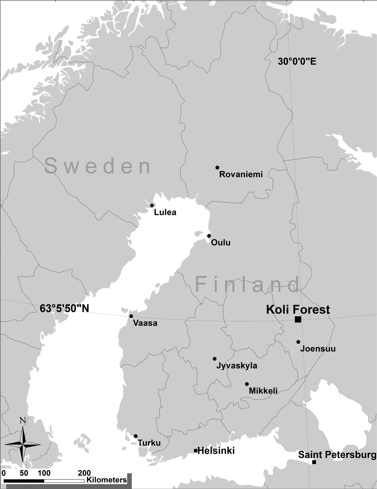
The study area is located about 340 m above sea level in Eastern Finland at the Koli Forest, which belongs to the Lieksa municipality (about 63°05′40″N, 29°48′31″E) (see Figure 1). The area is known for its white quartzite cliffs, steep topography and traditional landscapes. Over 70% of the region’s surface area is forest land, and 20% is water. The forest is dominated by conifers (65% pine, 25% spruce, 7% birch and 3% other species). The main tree species are Scots pine (Pinus sylvestris L.), and Norway spruce (Picea abies (L.) Karst). The area is sparsely populated with a total area of 21,585 km2 and a population of 175,000, which results in a population density of 9.8 inhabitants per square kilometer. Figure 1 shows a map of Finland and the location of the study site. The forests in the study site feature both natural and managed forests, with varying degrees of intensity. Conservation in the area is relatively young and was imposed less than twenty years ago. Both forest classes contain undergrowth.
Forest fires in Finland are mostly caught early on, because the country is still populated densely enough, and monitoring flights are frequent in the short hot season. However, as an example of neighboring Sweden from 2014 shows, strong winds and canopy fires can still be a devastating condition also in Finland.
2.2. Experimental Data
Two kinds of experimental data were used in this study, namely LiDAR data and field data. The following is a description of the data.
2.2.1. LiDAR Data
The LiDAR data used in this study were obtained free of charge from the National Land Survey (NLS) of Finland ( www.maanmittauslaitos.fi). The data were acquired in 2014 using an average flight altitude of 2 km with a scan angle of ±20 degrees. The resulting average LiDAR pulse density was 0.5 pulses per square meter, with an offset of approximately 1.4 m between the measurements. The mean error for height was 15 cm at most, while the horizontal accuracy was 60 cm. The beam footprint at ground level was 50 cm in diameter.
Information recorded for each LiDAR pulse includes the class of the pulse (ground or vegetation), flight line number, time stamp of the outgoing pulse, X-, Y- and Z-coordinates, intensity and the back-scattering order of the pulse. An automatic classification of the pulses into ground and vegetation returns was performed, and the results were checked against a stereo model from aerial imagery by the NLS.
LiDAR data used in the current article are of the same kind as the operational laser scanning of the forests in Finland. In 2010, Finland decided to scan the entire country by airborne laser in ten year cycles. The density chosen for this is roughly 0.5 returns per square meter. In the past, the scanners have mostly used single pulse mode, but currently, multiple pulse mode is widely adopted. As the goal of the current research is to calculate forest fire potential maps for the whole country, it has not been possible to adjust scanning parameters, such as pulse density.
2.2.2. Field Data
Field measurements for crown fuels were collected in April 2014 for 26 circular plots equally representing the dominant fuel types in the study area. Each plot covered an area of 256 m2 (radius = 9.03 m). A survey-grade Trimble GPS receiver was used to navigate to the plots and to georeference plot centers, acquiring data for plot centers from an average of at least 100 Global Navigation Satellite System (GNSS) locations.
Plot boundaries were measured using the Haglöff Vertex Laser Range Finder. The same instrument was used to measure the height of each tree. The diameter at breast height (DBH) was measured for all trees using a diameter tape. For each tree with a diameter at breast height (DBH) ≥ 8 cm in a plot, the following properties were recorded: tree class, species, DBH, height, crown base height (CBH) and crown class (dominant, co-dominant, intermediate and suppressed).
CBH was considered to be the distance between the ground and the lowest live branch in the crown of a tree. Small isolated branches with leaves, separated from the main crown, were not considered as indicating crown base height. The Haglöff vertex was used to measure CBH. The crown class of each tree was recorded as described above. Table 1 presents a summary of the field plots used as ground data.
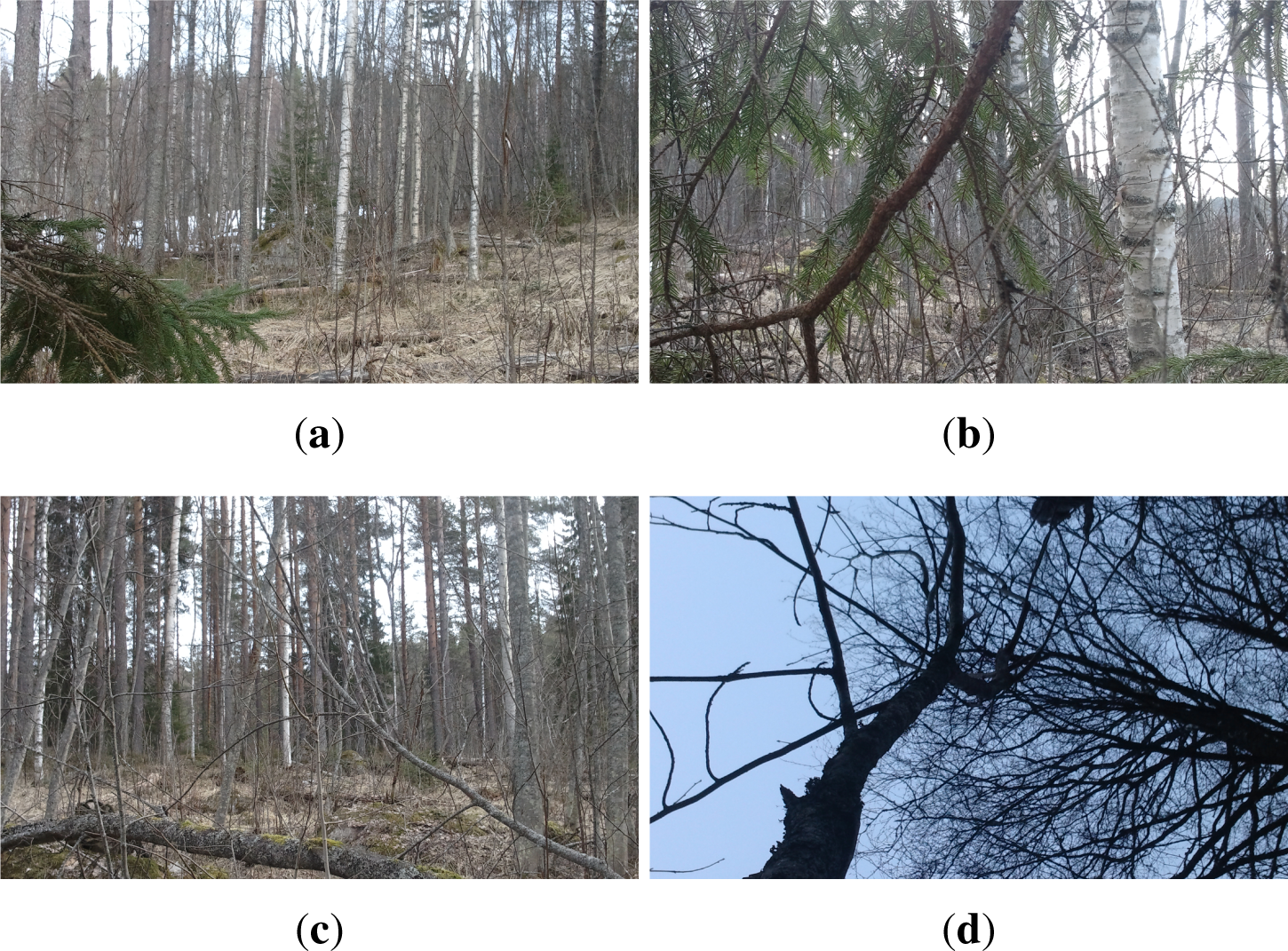
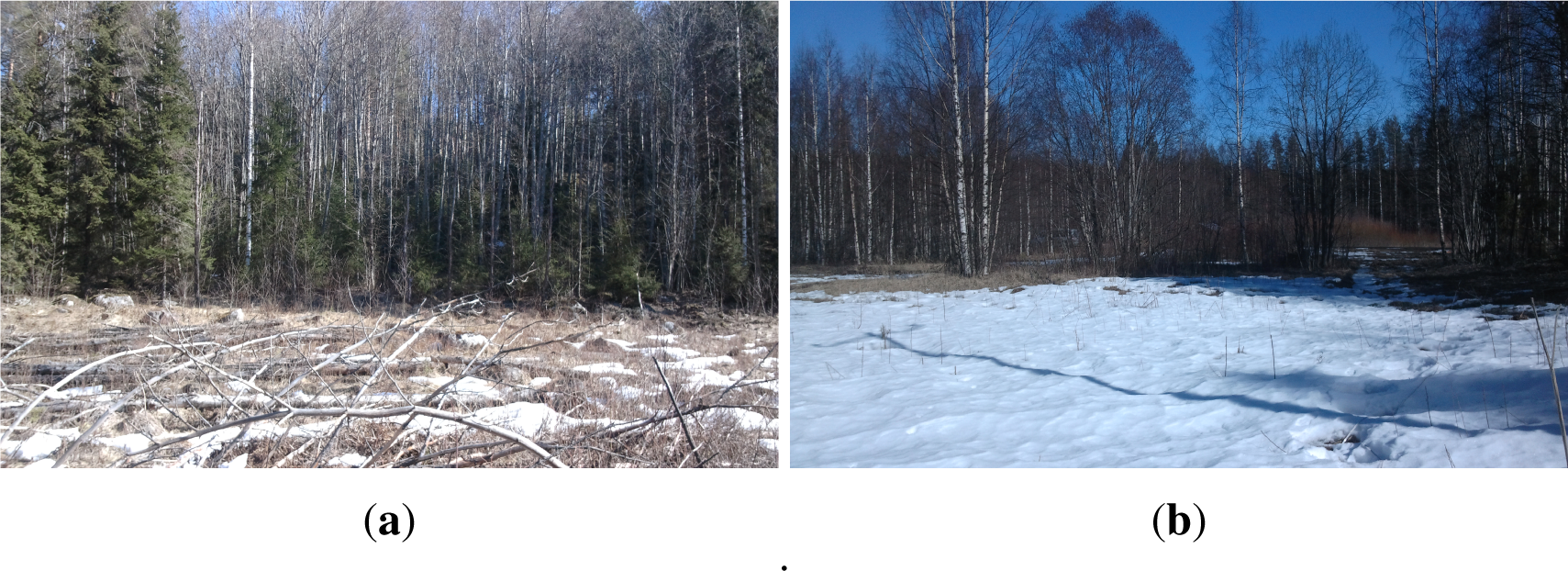
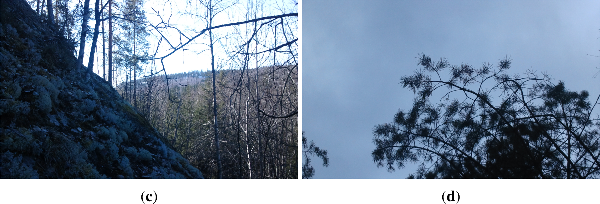
In addition to CBH measurements for individual trees in each plot, five pictures were taken from the plot center facing in the four cardinal directions (N, S, E, W) and the sky. These photos were taken to help as a visual aid later when analyzing and interpreting the experimental data. Figure 2 shows examples of plot photos.
2.3. Methods
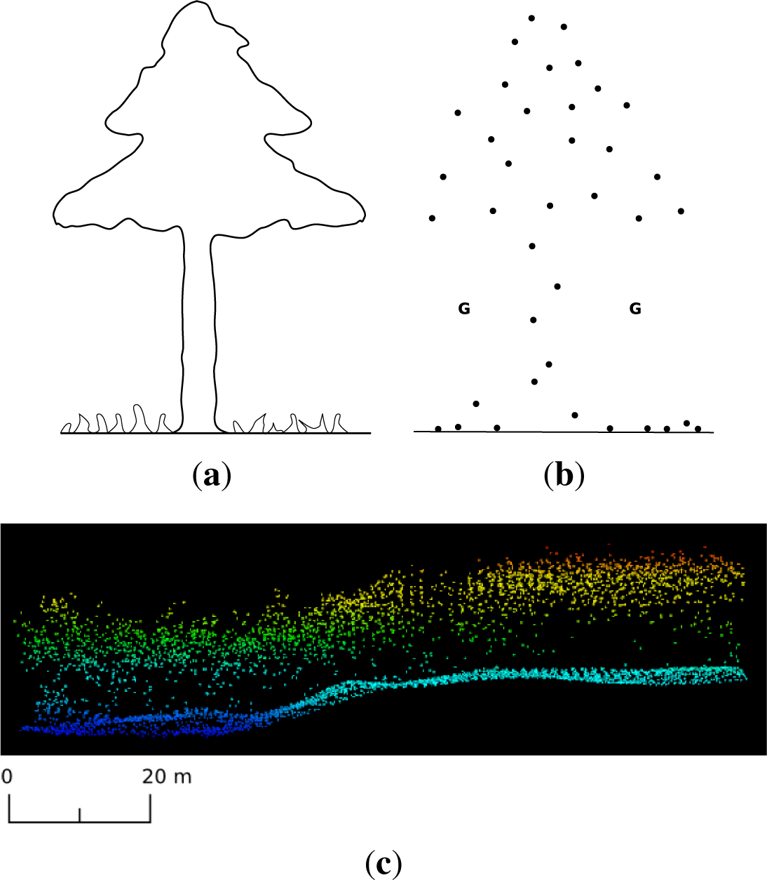
The method for estimating CBH from LiDAR data proposed in this paper is based on the idea of a moving voxel. A voxel, or volumetric pixel, is an analogy of a pixel in 3D. The use of the voxel in estimating CBH and other forest properties from LiDAR data has been reported in several past studies. In these studies, the emphasis had been to use the voxel to characterize the vertical structure of the canopy by dividing the LiDAR data into vertical bins (voxels) and counting the number of LiDAR hits in each bin (e.g., [34,35]). This paper takes a different approach and uses a moving voxel to locate gaps in the LiDAR point cloud (and hence, in the respective forest) and then estimates the height of these gaps from the ground. This information is then used to derive LiDAR metrics, which are used to estimate CBH as independent variables in a linear regression. The main assumption behind the method is that tree crowns tend to block most of the LiDAR pulses falling on them, thus creating a partial gap underneath the crown (see Figure 3). The idea is to use a moving voxel to locate gaps and estimate their height relative to the ground. It turns out that, as will be shown in the next section, the heights of these gaps strongly correlate with field-measured CBH values and are the basis for the LiDAR metrics used in estimating CBH in this paper.
To estimate CBH from LiDAR data, three main steps are performed: (1) initialization and data pre-processing; (2) searching for gaps and estimating their height (gap mapping); and (3) LiDAR metric generation and CBH estimation.
2.3.1. Initialization and Data Pre-Processing
The initialization and data pre-processing step sets the stage for subsequent steps. In this step, the LiDAR data are normalized, i.e., the elevation of every point is subtracted from the DTM of the area, so that each point represents height (from the ground), and then, all points with a height of less than 0.5 m (considered ground points) are discarded. Next, parameters governing the operation of the method are determined and initialized. These parameters include: voxel width, voxel height, step size and point threshold. Voxel width specifies the width and length of the voxel (i.e., the base), while voxel height specifies the height of the voxel. Step size specifies the distance (in meters) that the voxel moves horizontally (in the x–y plane), while point threshold specifies the maximum allowed number of points in a voxel to be considered a gap. Suitable values for these parameters for a given LiDAR point cloud are determined by experimenting on the field and LiDAR data. Values of these parameters used in this study were 8 m, 2 m, 1 m and 3 points for voxel width, voxel height, step size and point threshold, respectively. The choice of voxel width is influenced by point spacing in the LiDAR point cloud. If the width is too small relative to the point spacing, there will be too many false gaps, and if the width is too big, small gaps will be missed. Similarly, voxel height and step size are chosen, such that both small and large gaps are detected. Finally, if the point threshold is too small, very few gaps will be detected; if it is too high, there will be a large number of false gaps.
2.3.2. Gap Mapping
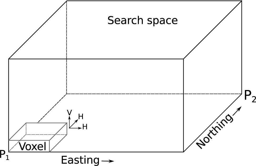
In this step, gaps in the LiDAR point cloud are located, and their heights relative to the ground are estimated. This is achieved by the use of a moving voxel in the search space. The search space is taken to be the box enclosing the pre-processed LiDAR point cloud with its origin at the point (Eastingmin, Northingmin, 0), where Eastingmin and Northingmin refer to the smallest easting and the smallest northing values in the point cloud, respectively (marked as P1 and P2, respectively, in Figure 4). Two kinds of movement are employed in the search space: (1) horizontal movement; and (2) vertical movement. Horizontal voxel movement is used to detect gaps, while vertical voxel movement is used to estimate the heights of the detected gaps.
Horizontal Voxel Movement
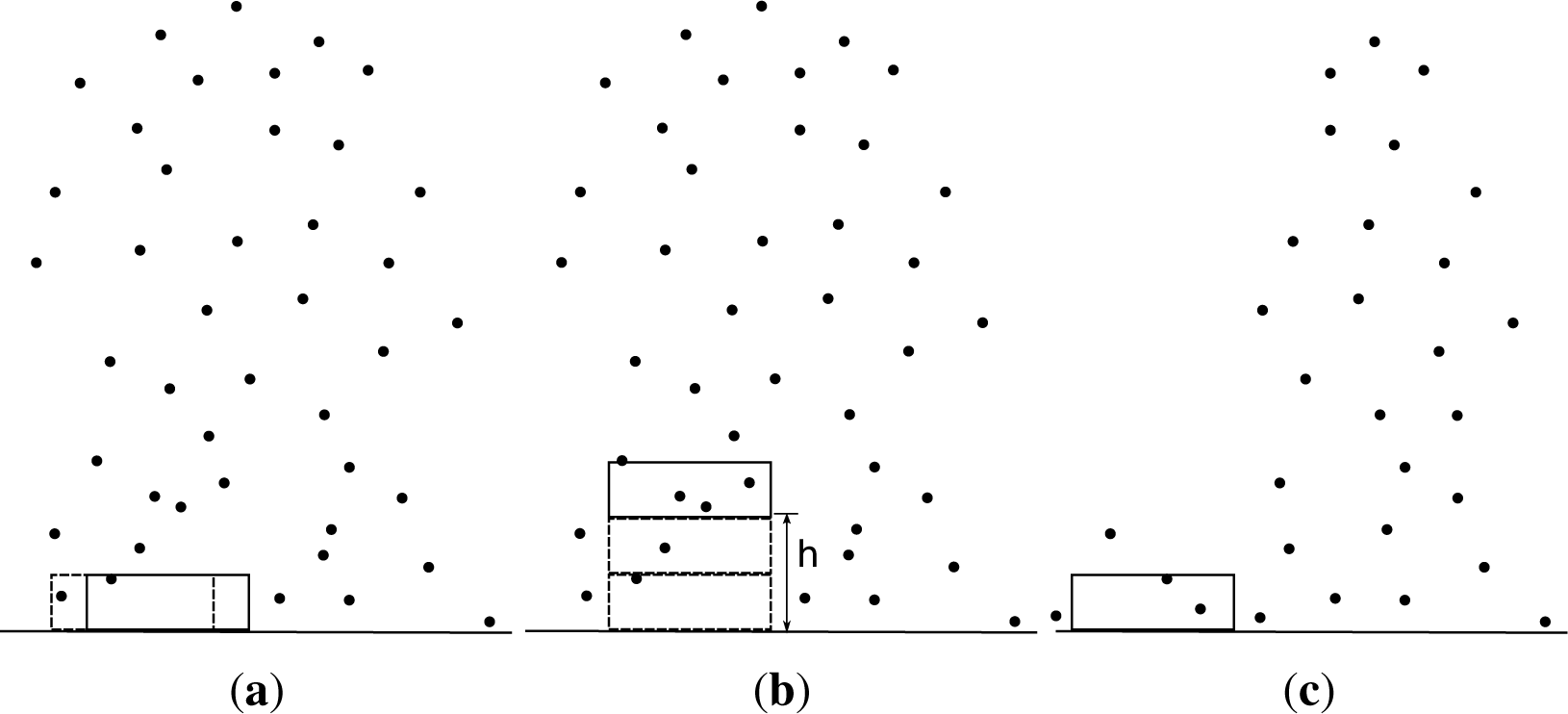
The goal of the horizontal voxel movement is to locate gaps in the search space. Starting at the origin of the search space, the voxel is first repeatedly moved along the x-axis (easting) using steps equal to the step size. At each step, points enclosed in the voxel are counted. A gap is detected when two conditions are met (see Figure 5): first, if the number of points in the voxel is less than or equal to the point threshold and, second, when the number of all of the points above the voxel is greater than the point threshold (see Figure 5a). The latter condition ensures that the gaps detected are not due to the absence of vegetation in the corresponding locations (see Figure 5c). After a gap has been detected, the next step is to estimate its height. This is achieved by using vertical voxel movement.
Vertical Voxel Movement
The aim of the vertical voxel movement is to estimate the heights of the gaps that have been detected. To estimate the height of a gap, the voxel is repeatedly moved upwards in steps equal to the voxel height until the number of points in the voxel exceeds the point threshold (see Figure 5). The height of the gap is then given by voxel height × N.
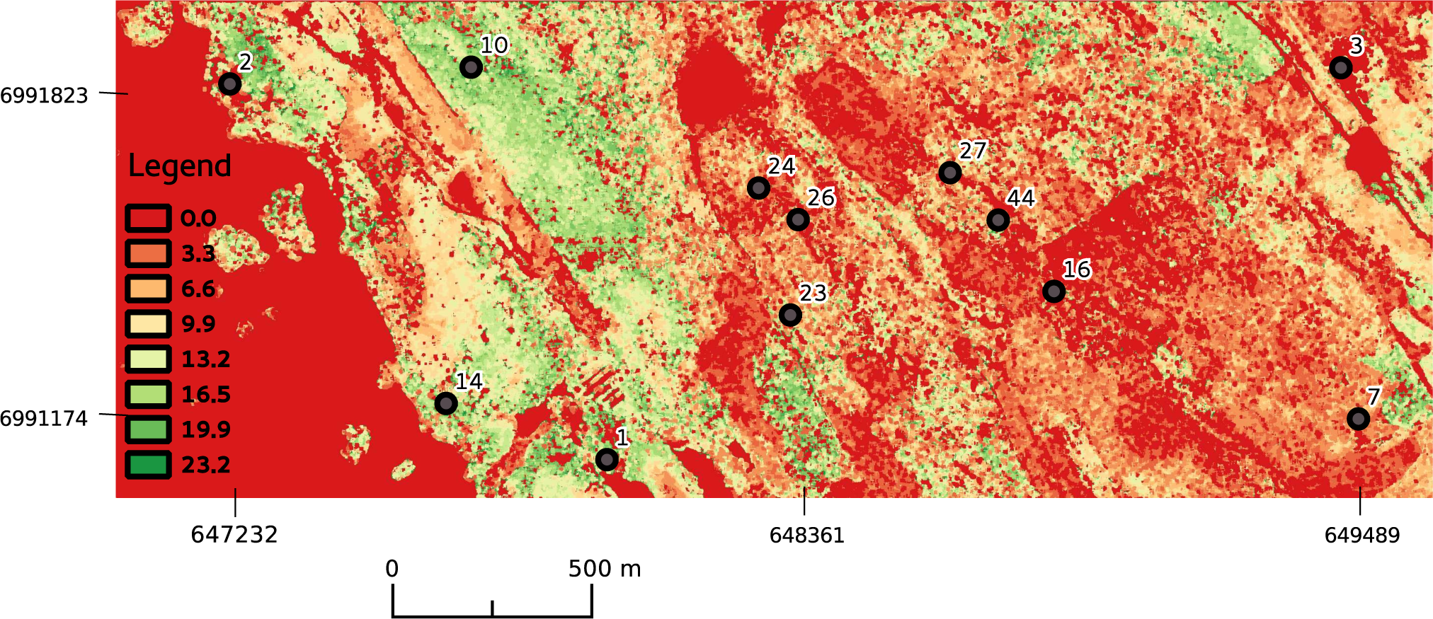
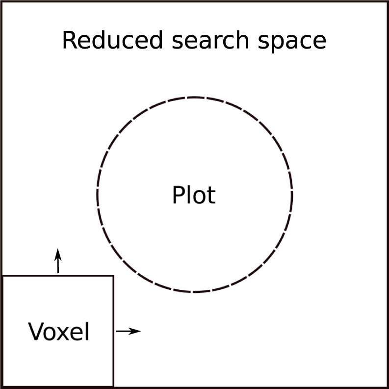
The outcome of the gap mapping step is a gap height raster with cell size equal to the step size and origin (top left corner) at ; note the starting point of the voxel in Figure 4. Figure 6 shows a portion of the gap height raster. Note that to speed up processing, searching for gaps can be confined to the space extending a few meters from the plot boundary, as shown in Figure 7.
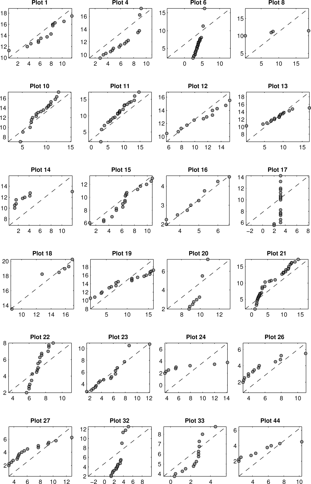
Figure 8 shows the degree of correlation between the estimated gap heights and the field-measured CBH values in 24 of the field plots. The plotted values for gap heights in each plot were obtained by taking the highest gap height values corresponding to the number of plots and matching them to the field-measured individual tree CBH values based on their magnitude (such that the highest goes with the highest, etc.). Plots with ID numbers 3 and 5 do not appear in the figure, because no information could be extracted from the LiDAR data corresponding to these plots. A possible reason for this anomaly is the fewer number of trees present in the plots (see Table 1 and Figure 9) and consequently fewer LiDAR points. Following this anomaly, subsequent analysis and results reported in the following sections are based on only the 24 plots shown in Figure 8.
2.3.3. LiDAR Metrics Generation and CBH Estimation
In this step, LiDAR metrics for use in CBH estimation (independent variables) are generated. These metrics are then combined with field-measured CBH values to form a dataset used for estimating CBH through linear regression.
LiDAR Metric Generation
To generate LiDAR metrics, the gap heights raster produced in the previous step is used. Points corresponding to each field-measured plot are extracted from the raster by taking all of the points that satisfy the equation:
Because of a small value for the step size used while generating the gap heights raster, there will be a high degree of duplication in the values extracted for each plot. Therefore, the next step is to remove duplicates from the values. To remove duplicates, the values are sorted (in either descending or ascending order) to bring equal values together into groups and picking one value from each group (see Figure 10). After duplicates have been removed, the following metrics (percentiles) are computed from the remaining values in each plot: g25, g50, g75 and g90. These metrics serve as independent variables for estimating CBH.
CBH Estimation
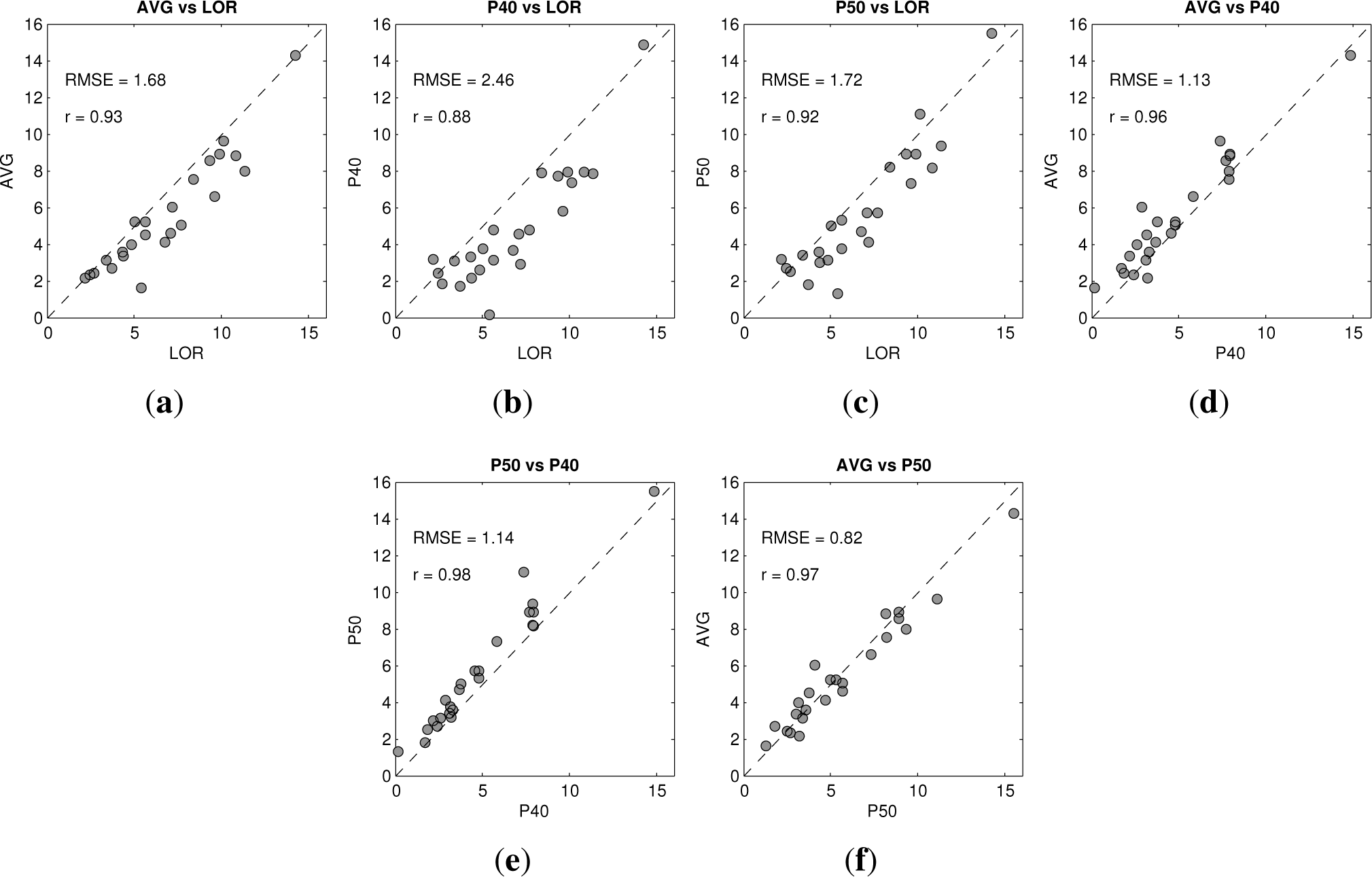
To estimate CBH, several regression models were fitted. For the purpose of model fitting, several variables representing CBH at the plot level were derived from the field data. These variables served as dependent variables in regression models and include: (1) Lorey’s mean (LOR); (2) the arithmetic mean (AVG); (3) the 40th percentile (P40); and (4) the 50th percentile (P50).
For comparison reasons, we fitted models using both the metrics introduced in this paper and traditional percentile LiDAR metrics (the coefficient of variation (CV), percentage of first returns, maximum height, mean height and the 25th, 50th, 75th and 90th percentiles) as independent variables.
Model fitting was done in the MATLAB™computing environment [36], whereby forward stepwise regression was used to automatically select variables for each model. Variable selection was based on the F-test. The minimum p-value for a variable to be removed was 0.1, while the maximum p-value for a variable to be added was set to 0.05. Leave-one-out cross-validation (LOOCV) was used to assess the predictive value of each regression model. For this purpose, the root mean squared error for cross-validation (RMSEcv) was used.
3. Results
CBH estimation results obtained by using the LiDAR metrics introduced in this paper as independent variables are shown in Table 2 and in Figure 11. Results obtained using traditional percentile LiDAR metrics as independent variables are shown in Figure 12 and in Table 3. The CBH estimation results using traditional percentile LiDAR metrics are based on [21]. In each case, the best model for each dependent variable (i.e., LOR, AVG, P40 and P50) obtained using stepwise regression is shown. The results shown in Table 3 were computed based on [21].
3.1. Effect of Voxel Width and Point Threshold
To study how the different dependent variables perform under various voxel dimensions and point thresholds, the effect of voxel dimensions was studied by varying the value of voxel width from 1 to 10 m, while keeping the point threshold and voxel height constant at three points and 2 m, respectively, and observing how the model RMSE for each dependent variable was affected. Similarly, The effect of point threshold was studied by varying the value of point threshold from 1–10 points. Figure 13 shows the effect of voxel width and point threshold on the model RMSE on the four dependent variables.
Results in Figure 13 show that LOR outperformed the other variables in both cases with lower and more consistent RMSE values in both cases. In the case of voxel width (Figure 13a), the best (more consistent) values for RMSE are obtained in the 5–8-m range. Outside this range, the RMSE values vary greatly among the variables. This behavior can be explained by the effect very large/very small voxels have. The effect of a large voxel for a given point threshold is that legitimate gaps will not be detected (false negatives), while the effect of a small voxel is that illegitimate gaps will be detected (false positives). For the LiDAR data used in this study, suitable values of voxel width are in the range 5–10 m. On the other hand, all four variable are affected in a similar manner with changes in point threshold (Figure 13b). Suitable values for point threshold in this case are those in the range of 3–6 points. These results further demonstrate the suitability of LOR for representing CBH at the plot level.
4. Discussion
Comparison of the four dependent variables (LOR, AVG, P40 and P50) showed that LOR gave the simplest model in either case (using traditional percentile LiDAR metrics and the proposed metrics) (see Tables 2 and 3). Furthermore, in both cases, the LOR-based model had the smallest RMSEcv, which was very close to the corresponding RMSE value. This implies that, in both cases, the LOR-based models have better predictive value over models based on the other dependent variables. This observation is in agreement with results reported in previous studies (e.g., [23]). This observation further supports the robustness of Lorey’s mean in CBH estimation over the commonly-used arithmetic mean. However, Lorey’s mean should be used with caution due to its tendency to be affected by big trees. This fact implies that in some cases, the CBH estimates obtained using Lorey’s mean may be higher than the actual CBH, that is the minimum canopy bulk density required for the propagation of a surface fire to the crown could be reached at a lower height than that estimated using Lorey’s mean.
With the exception of LOR, the remaining dependent variables gave more or less similar results in both cases, with higher RMSE and less consistent RMSEcv values being evident with models based on the traditional percentile LiDAR metrics. This similarity can be explained by the high degree of correlation among the variables, as shown in Figure 14. This observation implies that the use of different field estimates for CBH due to the lack of standardized field methods for estimating CBH does not have a profound effect on the final CBH estimation results. Despite this fact, LOR and AVG should be used with caution, because the former tends to be biased towards big trees, while the latter is susceptible to outliers. Point-cloud based voxels can also be seen as another way of defining CBH in a relatively objective way.
The lowest degree of correlation is seen between P40 and LOR (0.88) (Figure 14b), while the rest of the variable pairs exhibit higher correlation values of over 0.9. With this high level of correlation, it is expected that models based on either of these pairs of variables exhibit a high degree of similarity. In this respect, the two models based on the proposed metrics that used AVG and P50 as independent variables (Table 2) exhibited a higher degree of agreement compared to similar models using traditional percentile LiDAR metrics (see Table 3).
Performance of the models based on the traditional percentile LiDAR metrics (see Table 3) compares well with results obtained in previous studies (e.g., [21,34]), although there are significant differences in the number and type of independent variables in the models. For example, [21] used the same percentile LiDAR metrics for estimating CBH and obtained similar results (R2 = 0.77, RMSE = 3.9 and RMSEcv = 4.1), but some of the variables (coefficient of variation (CV) and percentage of first returns (D)) did not appear in the regression models reported in this paper. A possible explanation for this difference could be differences in the distribution (characteristics) of the LiDAR data used in the two studies, which, in turn, is affected by tree species and the season of data collection, among other factors. Conversely, models based on the proposed metric (see Table 2) gave better results based on all four criteria (RMSE, RMSEcv, R2 and p-value). These models had smaller RMSEs, higher R2 and smaller and more consistent RMSEcv values.
Although our results compare well with previous similar studies, the main limitation of this study is the small number of field sample plots used (24 plots), which is one possible source of model error. In contrast, previous studies have used significantly larger numbers of field sample plots (e.g., [21] (101 plots); [34] (62 plots); [23] (50 plots)). In another example, [37] used the Sparse Bayesian regression implemented in ArboLiDARTools [38] to build a linear model to estimate CBH from cumulative percentile variables of the LiDAR point cloud and validated the results with laser range-finding and a hypsometer on the ground in 250 sample plots. The RMSE of CBH estimated from LiDAR was 1.03 m.
With more sample plots, and therefore more redundancy in the training data, we anticipate better results also for the current method. Other possible sources of error include measurement error and instrument error.
5. Conclusions
This paper has proposed new LiDAR-based metrics for estimating CBH. Several field-based plot-level tree CBH variables, namely Lorey’s mean, arithmetic mean, the 40th and 50th percentiles, have been compared in order to find if there are any significant differences in using one variable over another.
Results obtained in this paper showed that the use of Lorey’s mean to estimate CBH leads to a slight improvement in accuracy compared to the other variables; no significant differences, however, were found among the rest of the variables. The use of Lorey’s mean over the other variables, however, will depend on the availability of the information required to compute Lorey’s mean, namely diameter at breast height (DBH). This is because Lorey’s mean is a weighted average with the basal area of individual trees as the weighting factor; therefore, bigger trees contribute more to the mean. However, since CBH is the minimum amount of fuel required to propagate the fire from the surface fuel layer to the canopy fuel layer, the use of Lorey’s mean has the potential to overestimate CBH due to the influence of bigger trees. This means the minimum canopy bulk density required to propagate surface fires into the crown can be reached at a lower height than the CBH obtained using Lorey’s mean. Therefore, based on this fact, Lorey’s mean should be used with caution.
The method for estimating CBH proposed in this paper gave better results (lower and more consistent RMSE and RMSEcv values and higher R2 values) compared to the use of traditional percentile LiDAR metrics, which have been widely used in previous studies. The main advantage of this method is that the metrics used for estimating CBH are derived from the estimated heights of gaps below trees as directly calculated from LiDAR data. The gap heights give an estimate of the distance of the lowest tree branches from the ground and correlate strongly with field-measured CBH values of individual trees. Moreover, a by-product of processing, which is a raster of gap heights, gives valuable information about the vertical structure of the forest stand below the canopy, i.e., which areas are closed (contain ladder fuels) and, hence, may need immediate attention (e.g., thinning), or identifying areas with low fuel volumes that could be modified to create a fuel break with relatively little manual labor and cost. On the other hand, the main limitation of the proposed method is that it is not suited for areas with pronounced understory layers (e.g., tropical rainforests). This is because the method is suited for detecting fuel breaks, which originate from the ground.
The method for estimating CBH from LiDAR data proposed in this paper gave better results over the use of traditional percentile LiDAR metrics; therefore, the method can potentially be applied to other fire-prone areas provided that suitable parameters are determined from the LiDAR data. The main limitation of the study was that the number of sample plots used (24) was relatively small compared to similar previous studies. Therefore, it would be interesting to conduct further tests on the method using larger numbers of sample plots in different kinds of forests and different seasons.
Acknowledgments
We would like to thank Arbonaut Finland Ltd. for the financial support it provided during the course of this study, which covered data collection, travel expenses and logistics.
Author Contributions
Almasi S. Maguya did the coding, data processing and wrote most of the article. Katri Tegel wrote Sections 2.1 and 2.2.1. Virpi Junttila and Tuomo Kauranne handled administrative issues, as well as proofreading the article. Markus Korhonen, Janice Burns, Vesa Leppanen and Blanca Sanz collected and pre-processed field data.
Conflicts of Interest
The authors declare no conflict of interest.
References
- Riebau, A.R.; Qu, J.J. Application of remote sensing and GIS for analysis of forest fire risk and assessment of forest degradation. In Natural Disasters and Extreme Events in Agriculture; Sivakumar, M., Motha, R., Das, H., Eds.; Springer: Berlin/Heidelberg, Germany, 2005; pp. 335–350. [Google Scholar]
- Montealegre, A.L.; Lamelas, M.T.; Tanase, M.A.; de la Riva, J. Forest fire severity assessment using ALS data in a mediterranean environment. Remote Sens. 2014, 6, 4240–4265. [Google Scholar]
- San-Miguel-Ayanz, J.; Moreno, J.M.; Camia, A. Analysis of large fires in European Mediterranean landscapes: Lessons learned and perspectives. For. Ecol. Manag. 2013, 294, 11–22. [Google Scholar]
- Pausas, J.G.; Llovet, J.; Rodrigo, A.; Vallejo, R. Are wildfires a disaster in the Mediterranean basin? A review. Int. J. Wildl. Fire 2008, 17, 713–723. [Google Scholar]
- Collins, R.D.; de Neufville, R.; Claro, J.; Oliveira, T.; Pacheco, A.P. Forest fire management to avoid unintended consequences: A case study of Portugal using system dynamics. J. Environ. Manag. 2013, 130, 1–9. [Google Scholar]
- European Communities. Forest Fires in Europe 2003; Technical Report SPI.04.124 EN; Institute for Environment and Sustainability, Official Publication of the European Communities: Brussels, Belgium, 2004. [Google Scholar]
- European Communities. Forest Fires in Europe 2005; Technical Report EUR 22 312 EN; Institute for Environment and Sustainability, Official Publication of the European Communities: Brussels, Belgium, 2006. [Google Scholar]
- European Communities. Forest Fires in Europe 2007; Technical Report EUR 2349 EN; Institute for Environment and Sustainability, Official Publication of the European Communities: Brussels, Belgium, 2008. [Google Scholar]
- NASA. Wildfire in Sweden: Image of the Day, Available online: http://earthobservatory.nasa.gov/IOTD/view.php?%20id=84155 accesed on 3 October 2014.
- Accuweather. Largest Wildfire in Over 40 Years Out of Control in Sweden, Available online: http://www.accuweather.com/en/weather-blogs/international/largest-wild-fire-in-over-40-years-out-of-control-in-sweden/31662445 accesed on 3 October 2014.
- Cui, X.; Gao, F.; Song, J.; Sang, Y.; Sun, J.; Di, X. Changes in soil total organic carbon after an experimental fire in a cold temperate coniferous forest: A sequenced monitoring approach. Geoderma 2014, 226–227, 260–269. [Google Scholar]
- Loehman, R.A.; Reinhardt, E.; Riley, K.L. Wildland fire emissions, carbon, and climate: Seeing the forest and the trees—A cross-scale assessment of wildfire and carbon dynamics in fire-prone, forested ecosystems. For. Ecol. Manag. 2014, 317, 9–19. [Google Scholar]
- Flannigan, M.; Amiro, B.; Logan, K.; Stocks, B.; Wotton, B. Forest fires and climate change in the 21st century. Mitig. Adapt. Strateg. Glob. Chang. 2006, 11, 847–859. [Google Scholar]
- Amiro, B.D.; Todd, J.B.; Wotton, B.M.; Logan, K.A.; Flannigan, M.D.; Stocks, B.J.; Mason, J.A.; Martell, D.L.; Hirsch, K.G. Direct carbon emissions from Canadian forest fires, 1959–1999. Can. J. For. Res. 2001, 31, 512–525. [Google Scholar]
- Oris, F.; Asselin, H.; Ali, A.A.; Finsinger, W.; Bergeron, Y. Effect of increased fire activity on global warming in the boreal forest. Environ. Rev. 2014, 22, 206–219. [Google Scholar]
- Agee, J.K.; Skinner, C.N. Basic principles of forest fuel reduction treatments. For. Ecol. Manag. 2005, 211, 83–96. [Google Scholar]
- Graham, R.T.; McCaffrey, S.; Jain, T.B. Science Basis for Changing Forest Structure to Modify Wildfire Behavior and Severity; Technical Report; USDA Forest Service, Rocky Mountain Research Station: Washington, DC, USA, 2004. [Google Scholar]
- Peterson, D.L.; Johnson, M.C.; Agee, J.K.; Jain, T.B.; Mckenzie, D.; Reinhardt, E.D. Fuels planning: Managing forest structure to reduce fire hazard, Proceedings of the 2nd International Wildland Fire Ecology and Fire Management Congress, Orlando, FL, USA, 16–20 November 2003; American Meteorological Society: Washington, DC, USA, 2003.
- Finney, M.A. FARSITE, Fire Area Simulator—Model Development and Evaluation; USDA: Washington, DC, USA, 2004. [Google Scholar]
- Arroyo, L.A.; Pascual, C.; Manzanera, J.A. Fire models and methods to map fuel types: The role of remote sensing. For. Ecol. Manag. 2008, 256, 1239–1252. [Google Scholar]
- Andersen, H.; McGaughey, R.J.; Reutebuch, S.E. Estimating forest canopy fuel parameters using LIDAR data. Remote Sens. Environ. 2005, 94, 441–449. [Google Scholar]
- Riaño, D.; Meier, E.; Allgöwer, B.; Chuvieco, E.; Ustin, S.L. Modeling airborne laser scanning data for the spatial generation of critical forest parameters in fire behavior modeling. Remote Sens. Environ. 2003, 86, 177–186. [Google Scholar]
- Agca, M.; Popescu, S.; Harper, C.W. Deriving forest canopy fuel parameters for loblolly pine forests in eastern Texas. Can. J. For. Res. 2011, 41, 1618–1625. [Google Scholar]
- Jain, T.B.; Graham, R.T. The relation between tree burn severity and forest structure in the Rocky Mountains. In Restoring Fire-Adapted Ecosystems: Proceedings of the 2005 National Silviculture Workshop; USDA Forest Service General Technical Report PSW-GTR-203; USDA: Washington, DC, USA, 2007; pp. 213–250. [Google Scholar]
- Cohen, J.D.; Butler, B.W. Modeling potential structure ignitions from flame radiation exposure with implications for wildland/urban interface fire management, Proceedings of the 13th Fire and Forest Meteorology Conference, International Association of Wildland Fire, Victoria, Australia, 27–31 October 1998; pp. 81–86.
- Rothermel, R.C. How to Predict the Spread and Intensity of Forest and Range Fires; Technical Report General Technical Report INT-143; Ogden, U.S. Department of Agriculture, Forest Service, Intermountain Forest and Range Experiment Station: Washington, DC, USA, 1983. [Google Scholar]
- Lemmens, M.; Airborne LIDAR. Geo-Information, Geotechnologies and the Environment; Gatrell, J.D., Jensen, R.R., Eds.; Springer Netherlands: Dordrecht, The Netherlands, 2011; Volume 5, pp. 153–170. [Google Scholar]
- Hudak, A.T.; Evans, J.S.; Stuart Smith, A.M. LiDAR utility for natural resource managers. Remote Sens. 2009, 1, 934–951. [Google Scholar]
- Keane, R.E.; Burgan, R.; van Wagtendonk, J. Mapping wildland fuels for fire management across multiple scales: Integrating remote sensing, GIS, and biophysical modeling. Int. J. Wildl. Fire 2001, 10, 301–319. [Google Scholar]
- Philip, M. Measuring Trees and Forests; CABI Publishing Series; CAB International: Wallingford, UK, 1994. [Google Scholar]
- Erdody, T.L.; Moskal, L.M. Fusion of LiDAR and imagery for estimating forest canopy fuels. Remote Sens. Environ. 2010, 114, 725–737. [Google Scholar]
- Van Wagner, C.E. Prediction of crown fire behavior in two stands of jack pine. Can. J. For. Res. 1993, 23, 442–449. [Google Scholar]
- González-Olabarria, J.; Rodríguez, F.; Fernández-Landa, A.; Mola-Yudego, B. Mapping fire risk in the Model Forest of Urbión (Spain) based on airborne LiDAR measurements. For. Ecol. Manag. 2012, 282, 149–156. [Google Scholar]
- Popescu, S.C.; Zhao, K. A voxel-based lidar method for estimating crown base height for deciduous and pine trees. Remote Sens. Environ. 2008, 112, 767–781. [Google Scholar]
- Chasmer, L.; Hopkinson, C.; Treitz, P. Assessing the three-dimensional frequency distribution of airborne and ground-based lidar data for red pine and mixed deciduous forest plots, Proceedings of the ISPRS Working Group VIII/2 “Laser-Scanners for Forest and Landscape Assessment”, Freiburg, Germany, 3–6 October 2004; XXXVI, pp. 66–70.
- MATLAB. The Matlab Computing Environment, Available online: http://www.mathworks.com/products/matlab accessed on 8 October 2014.
- Korhonen, M. Predicting Canopy Base Height (CBH) from Sparse Airborne LiDAR in a Scots Pine Dominated Forest and Enhancing the Efficiency of Field Measurements of CBH (in Finnish). Master’s Thesis, University of Eastern Finland, Savonlinna, Eastern Finland, Finland, 2012. [Google Scholar]
- Arbonaut Ltd. ArboLiDAR Forest Inventory–Automatic Stand Segmentation Manual, Proceedings of the ArboLiDAR User Days 2012 workshop, Joensuu, Finland, 2–4 October 2012; 2012.


| Plot ID | No. of Trees | DBH
| Height
| CBH
| ||||||
|---|---|---|---|---|---|---|---|---|---|---|
| Min | Max | Mean | Min | Max | Mean | Min | Max | Mean | ||
| 1 | 17 | 9.9 | 33.7 | 19.4 | 2.0 | 28.8 | 15.0 | 0.0 | 11.7 | 6.3 |
| 3 | 1 | 17.5 | 17.5 | 17.5 | 16.0 | 16.0 | 16.0 | 3.1 | 3.1 | 3.1 |
| 4 | 21 | 8.5 | 42.6 | 13.7 | 6.9 | 26.2 | 13.0 | 2.8 | 9.2 | 6.1 |
| 5 | 3 | 10.9 | 23.8 | 19.4 | 11.4 | 18.8 | 16.3 | 0.0 | 1.0 | 0.3 |
| 6 | 32 | 8.0 | 20.0 | 12.1 | 6.0 | 16.0 | 11.4 | 0.4 | 5.7 | 3.3 |
| 8 | 4 | 9.8 | 29.1 | 23.5 | 6.6 | 21.8 | 14.6 | 0.5 | 18.5 | 8.8 |
| 10 | 19 | 9.0 | 37.3 | 19.9 | 9.4 | 23.6 | 17.2 | 4.7 | 12.5 | 8.9 |
| 11 | 29 | 8.3 | 59.3 | 18.4 | 6.1 | 24.4 | 15.7 | 0.5 | 14.7 | 7.5 |
| 12 | 16 | 8.4 | 34.3 | 21.6 | 6.6 | 25.8 | 17.8 | 5.7 | 15.3 | 11.0 |
| 13 | 16 | 6.8 | 46.0 | 21.4 | 8.4 | 26.5 | 19.4 | 0.2 | 16.9 | 8.5 |
| 14 | 16 | 8.2 | 37.5 | 20.8 | 3.3 | 27.1 | 10.8 | 0.3 | 11.9 | 3.2 |
| 15 | 24 | 9.0 | 32.8 | 17.9 | 1.7 | 22.8 | 13.1 | 1.0 | 10.8 | 6.5 |
| 16 | 14 | 8.3 | 36.5 | 17.2 | 5.8 | 19.8 | 11.3 | 0.8 | 6.6 | 3.6 |
| 17 | 24 | 8.0 | 28.9 | 11.4 | 5.5 | 16.5 | 9.3 | 0.0 | 3.2 | 2.2 |
| 18 | 6 | 19.0 | 31.4 | 26.8 | 22.2 | 29.1 | 25.7 | 8.7 | 16.9 | 14.3 |
| 19 | 19 | 8.6 | 42.0 | 26.0 | 5.8 | 26.1 | 19.7 | 1.2 | 16.2 | 9.6 |
| 20 | 26 | 7.5 | 27.0 | 16.0 | 7.7 | 22.6 | 14.9 | 3.6 | 10.8 | 7.9 |
| 21 | 35 | 8.8 | 39.4 | 19.3 | 3.2 | 26.7 | 16.7 | 0.9 | 14.4 | 6.2 |
| 22 | 43 | 8.8 | 22.8 | 13.3 | 7.1 | 16.4 | 11.5 | 0.5 | 8.9 | 5.2 |
| 23 | 16 | 13.9 | 39.7 | 24.9 | 12.3 | 28.2 | 21.9 | 1.5 | 12.1 | 5.2 |
| 24 | 24 | 9.3 | 37.0 | 22.2 | 6.1 | 24.8 | 17.3 | 1.4 | 14.2 | 4.0 |
| 26 | 28 | 8.0 | 27.2 | 16.0 | 5.9 | 21.8 | 13.3 | 0.7 | 11.0 | 3.7 |
| 27 | 28 | 8.7 | 35.0 | 16.9 | 7.0 | 23.8 | 14.6 | 1.7 | 12.8 | 4.9 |
| 32 | 22 | 8.0 | 17.1 | 10.0 | 1.8 | 13.9 | 9.0 | 0.9 | 5.1 | 2.6 |
| 33 | 14 | 8.0 | 11.8 | 9.3 | 5.9 | 8.8 | 7.4 | 0.4 | 4.5 | 2.3 |
| 44 | 20 | 9.7 | 30.8 | 18.6 | 5.1 | 21.2 | 13.4 | 0.9 | 10.3 | 3.3 |
| Variable | CBH | RMSE (m) | RMSEcv (m) | R2 | p-value |
|---|---|---|---|---|---|
| LOR | (0.60)g75 + 0.79 | 2.40 | 2.69 | 0.46 | 0.003 |
| AVG | (1.05)g25 − (1.47)g50 + (1.06)g75 + 0.40 | 2.04 | 3.66 | 0.61 | 0.0003 |
| P40 | (1.28)g25 − (1.97)g50 + (1.98)g75 − (0.69)g90 + 1.20 | 1.74 | 3.36 | 0.75 | 0.00002 |
| P50 | (1.16)g25 − (1.82)g50 + (2.09)g75 − (0.75)g90 + 1.16 | 2.01 | 3.90 | 0.71 | 0.00006 |
| Variable | CBH | RMSE (m) | RMSEcv (m) | R2 | p-value |
|---|---|---|---|---|---|
| LOR | (0.56)h50 − 0.31 | 1.92 | 3.34 | 0.65 | 0.002 |
| AVG | (0.44)h50 − 0.07 | 2.31 | 3.51 | 0.44 | 0.0004 |
| P40 | (1.62)h50 − (1.19)h75 + 2.56 | 2.48 | 5.15 | 0.44 | 0.002 |
| P50 | (1.80)h50 − (1.26)h75 + 2.29 | 2.38 | 4.98 | 0.55 | 0.0002 |
© 2015 by the authors; licensee MDPI, Basel, Switzerland This article is an open access article distributed under the terms and conditions of the Creative Commons Attribution license (http://creativecommons.org/licenses/by/4.0/).
Share and Cite
Maguya, A.S.; Tegel, K.; Junttila, V.; Kauranne, T.; Korhonen, M.; Burns, J.; Leppanen, V.; Sanz, B. Moving Voxel Method for Estimating Canopy Base Height from Airborne Laser Scanner Data. Remote Sens. 2015, 7, 8950-8972. https://doi.org/10.3390/rs70708950
Maguya AS, Tegel K, Junttila V, Kauranne T, Korhonen M, Burns J, Leppanen V, Sanz B. Moving Voxel Method for Estimating Canopy Base Height from Airborne Laser Scanner Data. Remote Sensing. 2015; 7(7):8950-8972. https://doi.org/10.3390/rs70708950
Chicago/Turabian StyleMaguya, Almasi S., Katri Tegel, Virpi Junttila, Tuomo Kauranne, Markus Korhonen, Janice Burns, Vesa Leppanen, and Blanca Sanz. 2015. "Moving Voxel Method for Estimating Canopy Base Height from Airborne Laser Scanner Data" Remote Sensing 7, no. 7: 8950-8972. https://doi.org/10.3390/rs70708950