Optimized 3D Street Scene Reconstruction from Driving Recorder Images

Abstract

The paper presents an automatic region detection based method to reconstruct street scenes from driving recorder images. The driving recorder in this paper is a dashboard camera that collects images while the motor vehicle is moving. An enormous number of moving vehicles are included in the collected data because the typical recorders are often mounted in the front of moving vehicles and face the forward direction, which can make matching points on vehicles and guardrails unreliable. Believing that utilizing these image data can reduce street scene reconstruction and updating costs because of their low price, wide use, and extensive shooting coverage, we therefore proposed a new method, which is called the Mask automatic detecting method, to improve the structure results from the motion reconstruction. Note that we define vehicle and guardrail regions as “mask” in this paper since the features on them should be masked out to avoid poor matches. After removing the feature points in our new method, the camera poses and sparse 3D points that are reconstructed with the remaining matches. Our contrast experiments with the typical pipeline of structure from motion (SfM) reconstruction methods, such as Photosynth and VisualSFM, demonstrated that the Mask decreased the root-mean-square error (RMSE) of the pairwise matching results, which led to more accurate recovering results from the camera-relative poses. Removing features from the Mask also increased the accuracy of point clouds by nearly 30%–40% and corrected the problems of the typical methods on repeatedly reconstructing several buildings when there was only one target building.

1. Introduction

Due to the increasing popularity of using reconstruction technologies, more 3D supports are needed. Researchers have proposed many methods to generate 3D models. Building models from aerial images is a traditional method to reconstruct a 3D city. For example, Habib proposed a building reconstruction method from aerial mapping by utilizing a low-cost digital camera [1]. Digital map, Light Detection and Ranging (LIDAR) data, and video aerial image sequences have been used to build models combined [2]. These methods can reconstruct the model of large-area cities at a high efficiency; however, the models reconstructed from aerial data always have lacked detailed information, which constrains their further applications. In order to reconstruct city models with rich details, the terrestrial data based reconstruction also has been explored [3,4,5]; and street scenes have been reconstructed with imagery taken from different view angles [3,4]. These images were captured by a moving vehicle that carried a GPS/INS navigation system. Mobile LIDAR was used to reconstruct buildings with progressively refined point clouds by incrementally updating the data [5]. Even though mobile LIDAR can acquire 3D points quickly, it clearly has some limitations. For example, the density of the point clouds can be easily affected by the driving speeds, number of scanners, multiple returns, range to target, etc. The advantages and disadvantages of mobile LIDAR and its abundant applications in city reconstructions have been summarized [6]. The integrated GPS/Inertial Navigation Systems (INS) navigation system and mobile LIDAR play an important role in most classical city-scale reconstruction methods. However, in urban areas, the accuracy of GPS/GNSS is sometimes limited by the presence of large buildings. Although this limitation can be minimized by using Wi-Fi or telephone connections, we cannot neglect the necessity of INS in the above methods that has made city-scale reconstruction very expensive.

The urban area in China has grown rapidly in recent years, which has brought a large number of tasks for road surveying. However, the development of 3D street reconstruction is limited by the lack of mobile mapping equipment carrying stable GPS/INS systems or mobile LIDAR in China. In order to address this issue, it is crucial to be able to reconstruct sparse 3D street scenes without the assistance of GPS/INS systems. The Structure from Motion (SfM) technique [7] was recently used to reconstruct buildings from unstructured and unordered data sets without GPS/INS information [8,9], and the results should be scaled and georeferenced into object space coordinate systems. For example, the photo tourism system [10,11] is one of the typical SfM methods which can recover 3D point clouds, camera-relative positions, and orientations from either personal photo collections or Internet photos that do not rely on a GPS/INS system or any other equipment to provide location, orientation, or geometry. The image data used by the above typical SfM method characteristically have less repetition and obvious objects in the foreground, which allows processing by the typical SfM method have no additional steps.

With the heavier traffic density nowadays, especially more buses, taxis, and private vehicles are equipped with driving recorders to avoid traffic accident disputes. A driving recorder is a dashboard-mounted camera, which can collect images while a vehicle is operating. Figure 1 shows a typical driving recorder and recorded image.

Figure 1. Driving recorder and recorded image. (a) Photo of one type of driving recorder obtained from the Internet. (b) Test data recorded by the driving recorder in this paper.

Figure 1. Driving recorder and recorded image. (a) Photo of one type of driving recorder obtained from the Internet. (b) Test data recorded by the driving recorder in this paper.

More and more uses of driving recorders allow them to replace mobile mapping equipment to collect images, reconstruct, and update street scene point clouds at a lower cost yet in a shorter update time. Images of street views are typically captured by driving recorders mounted in the front of a moving vehicle, facing the forward direction along the street. Large quantities of vehicles are captured in the video images. However, due to the relative motion among the vehicles and the repeating patterns of guardrails, without the assistance of GPS/INS information, the matching pairs of images of vehicles and guardrails may be outliers. These outliers often take a dominant position, which cannot be removed by the epipolar constraint method effectively, thereby causing the typical SfM process to fail. Hence, this paper mainly focuses on detecting vehicles and guardrail regions, and then removing the feature points on them to reduce the number and negative effects of the outliers present in the driving recorder data. After removal, the remaining points can be used to reconstruct the street scene.

In order to reduce the cost of reconstructing point clouds, the SfM method is proposed in this paper to reconstruct the street scene based on driving recorder images without GPS/INS information. However, we reconstruct the results only in the relative coordinate system, rather than georeferencing it to the absolute coordinates. This paper focuses on removing the feature points on the vehicle and guardrail regions, which can improve the performance of the recovered camera-tracks and the accuracy of the reconstructed sparse 3D points. Vehicle and guardrail region automatic detection methods are proposed in Section 2.1, Section 2.2, Section 2.3 and Section 2.4. The features removing and reconstruction method is described in Section 2.5; and the improved reconstruction effects are shown in Section 3 from the following three aspects: Section 3.2 addresses the precision of pairwise orientation; Section 3.3 shows the camera poses recovering results, and the sparse 3D point clouds reconstructing results are introduced in Section 3.4. The results and implications of this research are discussed in Section 4; and the limitations of the proposed method and future research directions are described in Section 5.

2. Methodology

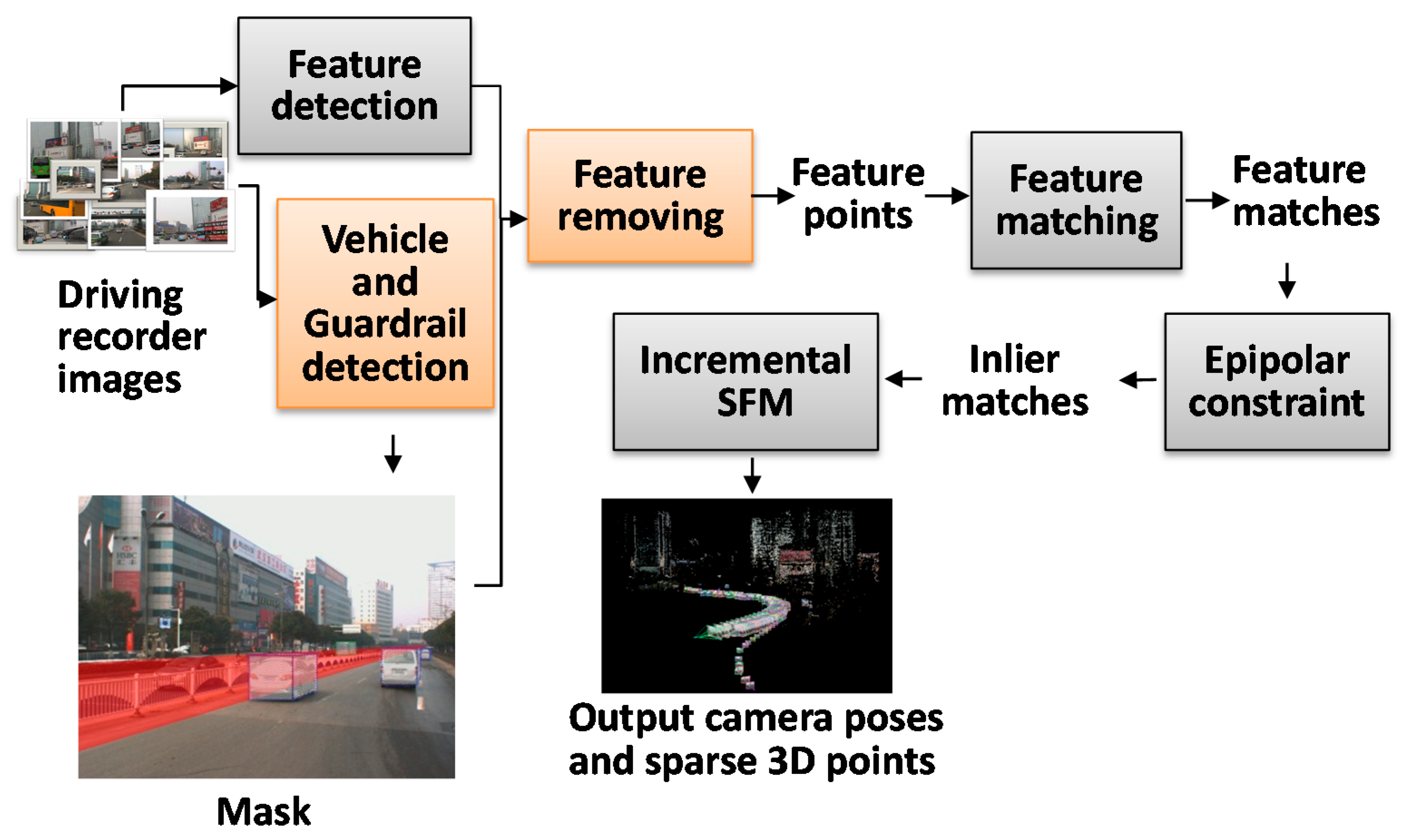
The paper proposed guardrail and vehicle region detection methods, and then masked feature points on guardrail and vehicle regions to improve the reconstruction result. We propose to “mask” out the vehicle and guardrail regions before reconstruction because guardrails have repeating patterns and vehicles move between frames, which subsequently always produce outliers on the image of the guardrail and vehicle regions. In this paper, the images of the vehicle and guardrail regions are collectively called the Mask. The pipeline of 3D reconstruction that utilizes driving recorder data is illustrated in Figure 2. We can first detect the SIFT [12] feature points and the Mask in each image, and then we remove the features on the Mask and match the remaining feature points between the pairs of images. Based on the epipolar constraint [7], we will remove the outliers to further refine the results and finally conduct an incremental SfM procedure [7] to recover the camera parameters and sparse points.

Figure 2. The pipeline of 3D reconstruction from driving recorder data. The grey frames show the typical SfM process. The two orange frames are the main improvement steps proposed in this paper.

Figure 2. The pipeline of 3D reconstruction from driving recorder data. The grey frames show the typical SfM process. The two orange frames are the main improvement steps proposed in this paper.

It is challenging to detect the Mask with object detection methods due to the following difficulties:

• Both the cameras and the objects are in motion, which changes the relative pose of the objects. Moreover, the appearance of vehicles varies significantly (e.g., color, size, and difference between back/front appearances).
• The environment of the scene (e.g., illumination and background) often changes, and events such as occlusions are common.
• Guardrails are strip distributions on images, which make the detection of whole regions difficult.

Haar-like features [13,14] based on Adaboost classifiers [15] were used to address the above challenges. With the help of classifiers, the front/back surfaces of vehicle and some parts of guardrails are automatic detected within a few seconds. The classifiers also could robust against the changing of light condition and environment.

In order to diminish the adverse impact of outliers on reconstruction, the Mask requires detection as entirely as possible. Therefore, based on the typical vehicle front/back surface detection method in Section 2.1, the design of the vehicle side surfaces detection method and the blocked-vehicle detection method are described in Sections 2.2 and Section 2.4, respectively. The blocked-vehicle is a vehicle moving in the opposite direction partially overlapped by the guardrail. The guardrail region detection method is introduced in Section 2.3, which is based on the Haar-like classifiers and the position of the vanishing point. Finally, the Mask and the reconstruction process are introduced in Section 2.5.

2.1. Vehicle Front/Back Surfaces Detection

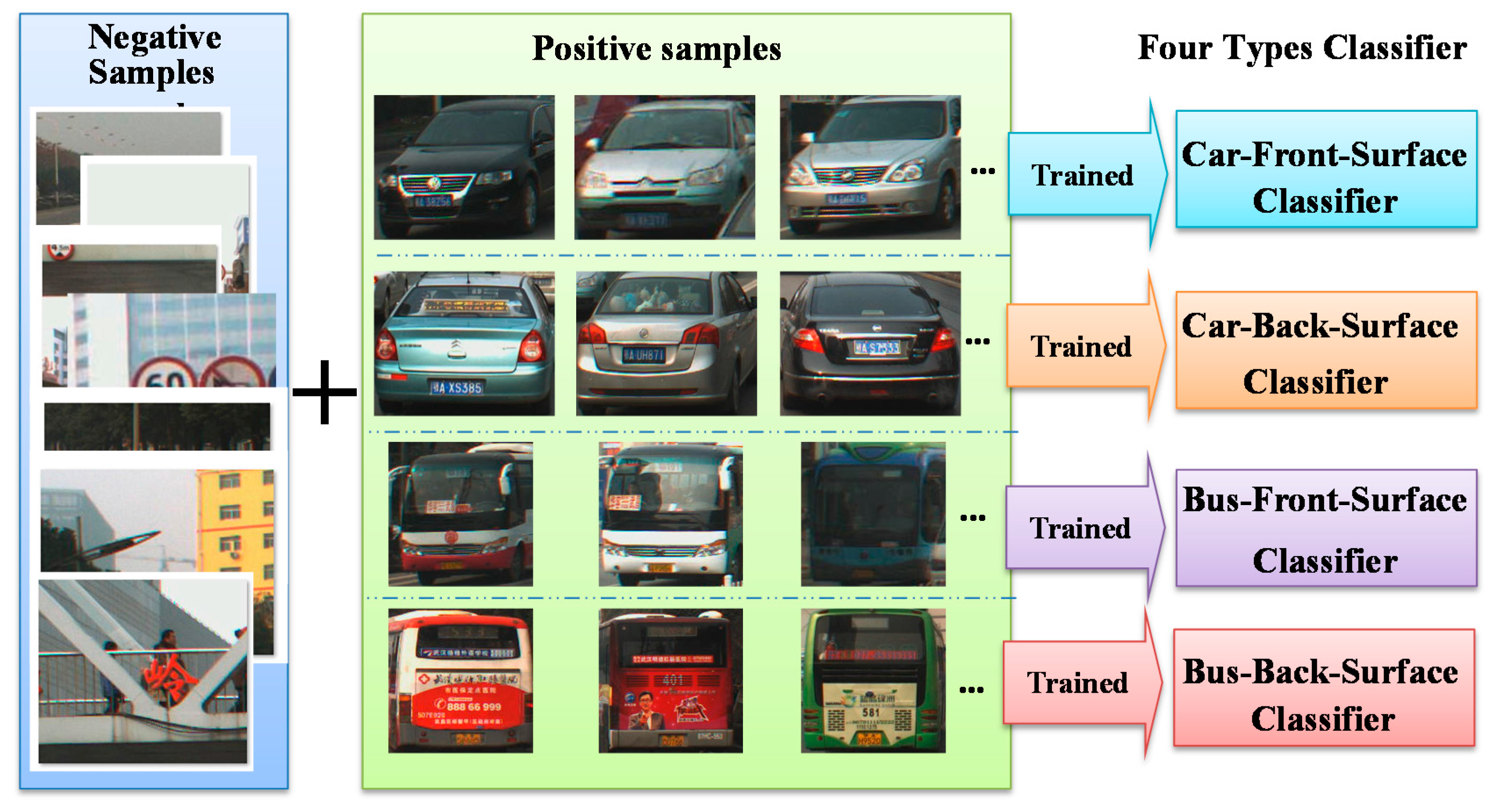
As the system of vehicle back surface detection [16] by Haar-like feature-based Adaboost classifier is described in details, we only summarize its main steps here. Classifiers based on Haar-like features can detect objects with a similar appearance. There is a big difference between the front and back surfaces of vehicles and buses; therefore, four types of classifiers were trained to detect the front and back surfaces of vehicles and buses, respectively.

The classifier was trained with sample data. After the initial training, the trained classifier was used to independently detect vehicles. There are two types of samples, positive and negative. A positive sample is a rectangular region cut from an image that contains the target object, and a negative sample is a rectangular region without the target object. Figure 3 shows the relation of the four classifier types and their trained samples. Each classifier is trained with 1000–2000 positive samples and at least 8000 negative samples. All the samples were manually compiled; and we separated the images containing vehicles as positive samples and the remaining images were used as negative samples. Although diverse samples can produce better classifier performance, a small amount of duplications are acceptable. Therefore, the positive samples of the same vehicle cut from different images are effective samples, and the samples from the same images with a slightly adjusted position are allowable as well. Two samples can even be totally duplicated, which will have a minimal adverse effect on the performance of the classifier when the number of samples is large enough. After inputting the samples into the OpenCV 2.4.9 [17] training procedure, the classifier can be trained with the default parameters automatically. A cascade classifier is composed of many weak classifiers. Each classifier is trained by adding features until the overall samples are correctly classified. This process can be iterated up to construct a cascade of classification rules that can achieve the desired classification ratios [16]. Adaboost classifier is more likely to overfit on small and noisy training data. Too many iterative training processes may cause the overfitting problem, too. Therefore, we need to control the maximum number of iteration in the training processes. In OpenCV training procedure, there are some constraints designed to avoid the overfitting problem. For example, the numStages parameter limits the stage number of classifier, and the maxWeakCount parameter helps to limit the count of trees. These parameters could prevent classifiers from the overfitting. Besides these parameter-constraints, we can also use more training data to minimize the possibility of overfitting.

Figure 3. Example of samples and classifiers.

Figure 3. Example of samples and classifiers.

A strong cascade classifier consists of a series of weak classifiers in the order of sparse to strict. A sparse classifier has few constraints and low classification accuracy but a high computational speed; while a strict classifier has many constraints and high classification accuracy but a low computational speed. When an image area is input into a strong cascade classifier, it is first detected by the initial sparse classifier. Only a positive result from the previous classifier triggers the evaluation of the next classifier. Negative results (e.g., background regions of the image) therefore are quickly discarded so the classifier can spend more computational time on more promising object-like regions [13]. Most image areas without the target object can be easily identified and eliminated at the very beginning of the process with minimal effort. Therefore, a cascade classifier is able to enhance computational efficiency [18].

2.2. Vehicle Side-Surface Detection

The side-surfaces of vehicles cannot be detected by feature-based classifiers since a vehicle’s appearance changes with the angle of view. Poor matching points on these regions inevitably have adverse effects on the reconstruction, especially the side-surfaces of large vehicles that are close to the survey vehicle.

The side-surface region can be determined if the interior orientation parameters, the rough size of the vehicles, and the position of the front/back surfaces of vehicles on the images are known. However, most driving recorders do not contain accurate calibration parameters so we deduced the equations described in this section to compute the rough position of the vehicle side-surface region based on the position of the front/back-surfaces and the vanishing point in the image, the approximate height H of the recorder, the rough value of focal length f, and the pitch angle of recorder $\text{θ}$. The vanishing point used in this section was located using the [19,20] method and the position of the vehicle front/back-surface was detected with the method described in Section 2.1. The vanishing point is considered a point in the picture plane that is the intersection of a set of parallel lines in space on the picture plane. Although the vehicle side-surface detection method proposed in this section can only locate the approximate position of the vehicle side-surface, it is adequate for masking out the features on vehicles to improve the reconstruction results. The length of M″N″ is the key step in the vehicle side-surface detection method. The process of computing the length of M″N″ is described below:

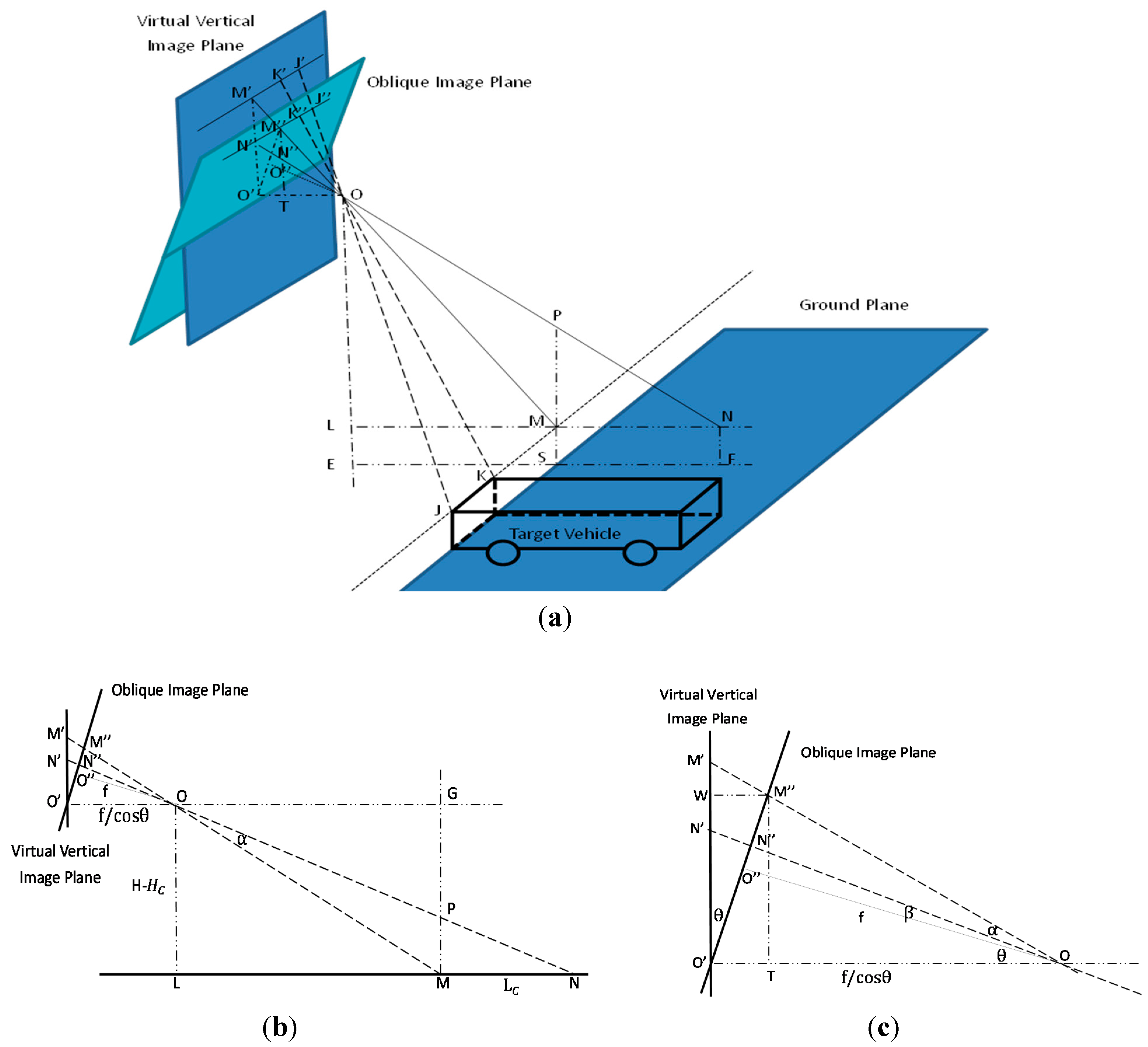
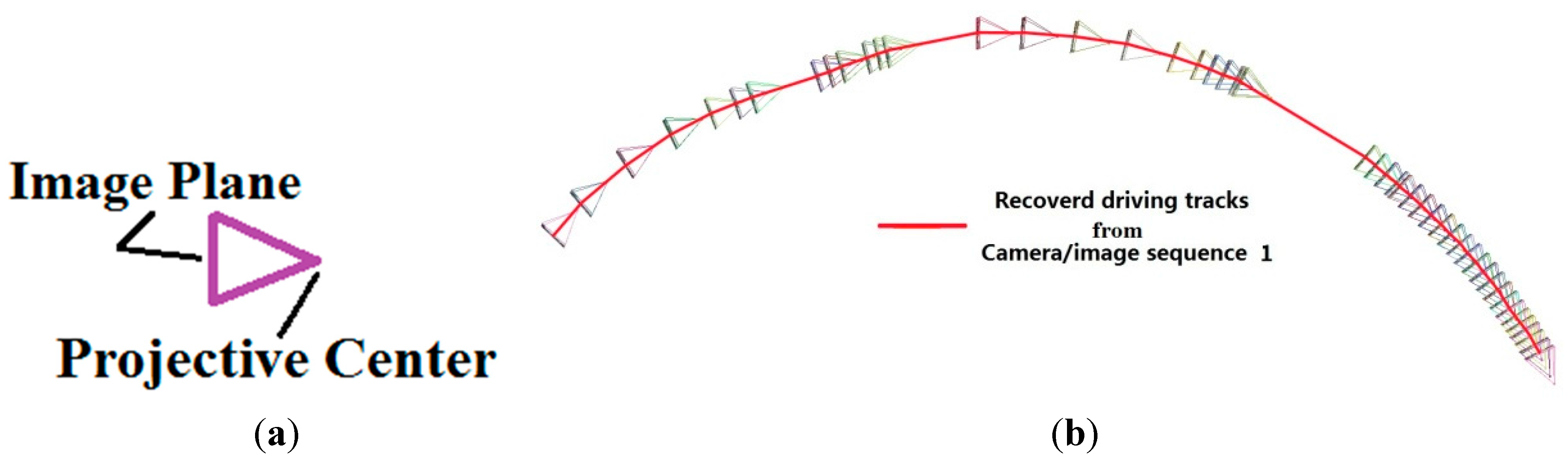
Figure 4. Photographic model of driving recorder. (a) Integrated photographic model of driving recorder. (b) Side view of model. (c) Partial enlargement of side view model. The oblique image plane is the driving recorder image plane. Point O is the projective center, and $\text{O″}$ is the principal point on the driving recorder image plane. The focal length f is $\text{OO″}$. Point $\text{O′}$ is the principal point on the virtual vertical image plane. Line OE is perpendicular to the ground. Point E is the intersection point of the ground and line OE. The plane $\text{M′O′}$OOEF can be drawn perpendicular to both the image plane and the ground. $\text{OM′}$ is perpendicular to $\text{M′J′}$, and OM is perpendicular to MJ. Line LN is perpendicular to OE. MP is a vertical line for the ground, and P is the intersection point of line MP and line ON. Line $\text{M″}$T is perpendicular to $\text{O′O}$. The angle between the oblique plane and the vertical plane is $\text{θ}$. Angles MON and $\text{O″ON″}$ are $\text{α}$ and $\text{β}$, respectively.

Figure 4. Photographic model of driving recorder. (a) Integrated photographic model of driving recorder. (b) Side view of model. (c) Partial enlargement of side view model. The oblique image plane is the driving recorder image plane. Point O is the projective center, and $\text{O″}$ is the principal point on the driving recorder image plane. The focal length f is $\text{OO″}$. Point $\text{O′}$ is the principal point on the virtual vertical image plane. Line OE is perpendicular to the ground. Point E is the intersection point of the ground and line OE. The plane $\text{M′O′}$OOEF can be drawn perpendicular to both the image plane and the ground. $\text{OM′}$ is perpendicular to $\text{M′J′}$, and OM is perpendicular to MJ. Line LN is perpendicular to OE. MP is a vertical line for the ground, and P is the intersection point of line MP and line ON. Line $\text{M″}$T is perpendicular to $\text{O′O}$. The angle between the oblique plane and the vertical plane is $\text{θ}$. Angles MON and $\text{O″ON″}$ are $\text{α}$ and $\text{β}$, respectively.

In Figure 4a, we suppose that the real length, height, and width of the vehicle are ${\text{L}}_{\text{C}}$, ${\text{H}}_{\text{C}}$ and ${\text{W}}_{\text{C}}$, respectively. The width of the target on image $K\text{″J″}$ is ${\text{W}}_{\text{P}}$. H is the height of projective center O to ground OE. Therefore, it can be seen that the length of target MN is ${\text{L}}_{\text{C}}$, the length of LE is ${\text{H}}_{\text{C}}$ and OL is H − ${\text{H}}_{\text{C}}$. Figure 4a shows that triangle $\text{M″}$TO is similar to OLM and triangle $K\text{″J″}$ O is similar to KJO. We therefore can deduce the following equations from the triangle similarity theorem:

$$\frac{K\text{″J″}}{KJ}=\frac{OM\text{″}}{OM}=\frac{M\text{″}T}{OL}$$

(1)

So the length of $\text{M″T}$ can be described with Equation (2):

$$\text{M″T}=\frac{K^{″}{J}^{″}·OL}{KJ}=\frac{W_P·\left(\text{H}-H_C\right)}{W_C}$$

(2)

It can be seen from △W $\text{OM′}$ in Figure 4c that, angle W $\text{O′M′}$ is $\text{θ}$, and the length of $\text{WM″}$ is equal to $\text{O′T}$ in rectangle $\text{WM″} \text{TO′}$. Then, Equation (3) can be established with the length of $\text{M″T}$ in Equation (2):

$$\text{WM″}=M\prime \prime T·tan\text{θ}=\frac{W_P·\left(\text{H}-H_C\right)·tan\theta }{W_C}$$

(3)

In Figure 4c, the length of $\text{M″T}$ is equal to W $\text{O′}$ in rectangle $\text{WM″} \text{TO′}$, so the length of $\text{M′O′}$ is equal to M″T add $\text{M′W}$. Then, Equation (4) can be established based on △ $\text{M′ WM″}$ ∽△ $\text{M′ O′O}$:

$$\frac{WM\prime \prime }{O\prime O}=\frac{M\prime W}{M\prime O\prime }=\frac{M\prime W}{M^{″}T+M\prime W}$$

(4)

Equation (5) is transformed from Equation (4), and the length of $\text{M′W}$ is expressed below:

$$\text{M′W}=\frac{WM\text{″}·M\text{″}T}{O^{\prime }O-WM\text{″}}=\frac{{W_P}^2·{\left(\text{H}-H_C\right)}^2·sin\theta }{{W_C}^2·f-W_P·W_C·\left(\text{H}-H_C\right)·sin\theta }$$

(5)

Equation (6) is established from rectangle $\text{WM″} \text{TO′}$ in Figure 4c.

$$\text{O′ M′}=\text{O′ W}+\text{M′ W}=\text{M′′ T}+\text{M′ W}=\frac{W_p·(\text{H}-H_c)}{W_c}+\frac{{W_P}^2·{\left(\text{H}-H_C\right)}^2·sin\theta }{{W_C}^2·f-W_P·W_C·\left(\text{H}-H_C\right)·sin\theta }$$

(6)

In Figure 4a, since $\text{OM″}$ is the height of triangle $\text{OK″J″}$, we can infer that:

∵△K’J’O∽△K’’J’’O, △OM’’T∽△OM’O’

(7)

$$\text{∴}\frac{K\text{′}J\text{′}}{\text{K″J″}}=\frac{OM\text{′}}{OM\text{″}}=\frac{O\text{′}M\text{′}}{M\text{″}T}$$

(8)

We know that, $K\text{″}J\text{″}$ is ${\text{W}}_{\text{P}}$, therefore with the calculations of M″T (Equation (2)) and O′M′ (Equation (6)), the length of $\text{K′J′}$ can be established from the transformation of Equation (8):

$$\text{K′J′}=\frac{K^{″}{J}^{″}·O\text{′}M\text{′}}{M\text{″}T}=W_P+\frac{{W_P}^2·\left(\text{H}-H_C\right)·sin\theta }{W_C·f-W_P·\left(\text{H}-H_C\right)·sin\theta }$$

(9)

KJ and $\text{K′J′}$ are parallel; therefore, we can infer that triangle $\text{K′} \text{M′}$O and triangle KMO are similar triangles from Figure 4a. $\text{ OM′}$ is the height of triangle $\text{K′} \text{M′}$O and OM is the height of triangle KMO. Meanwhile, $\text{OO′}$ and LN are parallel lines so triangle $\text{M′OO′}$ is similar to triangle OML. Therefore, based on the triangle similarity theorem, Equation (10) can be established:

$$\frac{K\prime J\prime }{KJ}=\frac{OM\prime }{OM}=\frac{OO\prime }{LM}$$

(10)

The length of $\text{OO′}$ is $\text{f}/\text{cosθ }$ and KJ is ${\text{W}}_{\text{C}}$ so LM can be calculated based on Equations (9) and (10):

$$\text{LM}=\frac{\text{OO′}·\text{KJ}}{K\text{′}J\text{′}}=\frac{W_C·f-W_P·\left(\text{H}-H_C\right)·sin\theta }{W_P·cos\theta }$$

(11)

In Figure 4b, Equation (12) can be established since triangle PMN is similar to OLM:

$$\frac{MP}{OL}=\frac{MN}{LN}=\frac{MN}{LM+MN}$$

(12)

OL and MN are H − ${\text{H}}_{\text{C}}$ and ${\text{L}}_{\text{C}}$, respectively. Then, MP can be described with Equations (11) and (12)

$$\text{MP}=\frac{OL·MN}{LM+MN}=\frac{L_C·W_P·\left(\text{H}-H_C\right)·cos\text{θ}}{W_C·f-W_P·\left(\text{H}-H_C\right)·sin\text{θ}+L_C·W_P·cos\text{θ}}$$

(13)

In order to compute the length of M’’N’’, we suppose that:

$$\angle {\text{M′ON}}^{\text{′}}=\angle \text{MON}=\text{α},\angle {\text{N″OO}}^{\text{″}}=\text{β},\angle \text{M′O′M″}=\angle \text{O′OO″}=\text{θ}$$

(14)

Based on cosine theorem, Equation (15) can be established:

$$\text{cosα}=\frac{O{P}^2+O{M}^2-M{P}^2}{2·OP·OM}$$

(15)

In Figure 4b, OG is equal to LM, and OL has the same length as GM in rectangle OGML. The length of OL is H − ${\text{H}}_{\text{C}}$. Based on the Pythagoras theorem, Equations (16) and (17) were deduced from △OGP and △OLM.

$$O{P}^2=O{G}^2+G{P}^2=L{M}^2+{(OL-MP)}^2=L{M}^2+{(\text{H}-{\text{H}}_{\text{C}}-MP)}^2$$

(16)

$$O{M}^2=O{L}^2+L{M}^2={\left(\text{H}-{\text{H}}_{\text{C}}\right)}^2+L{M}^2$$

(17)

Taking Equations (16) and (17) into Equation (15), angle $\text{α}$ can be described as follow:

$$\text{α}=\text{arccos}(\frac{L{M}^2+{\left(\text{H}-H_C\right)}^2-\left(\text{H}-H_C\right)·MP}{\sqrt{L{M}^2+{\left(\text{H}-H_C-MP\right)}^2}·\sqrt{{\left(\text{H}-H_C\right)}^2+L{M}^2}})$$

(18)

In Figure 4b,c, $\angle {\text{M′OO}}^{\text{′}}=\angle \text{OML}=\text{α}+\text{β}+\text{θ }$ so in triangle OML:

$$\tan \left(\text{α}+\text{β}+\text{θ}\right)=\frac{OL}{LM}$$

(19)

Equation (20) is the transformation of Equation (19), with OL= H− ${\text{H}}_{\text{C}}$:

$$\text{β}=\arctan \left(\frac{\text{H}-H_C}{LM}\right)-\text{α}-\text{θ}$$

(20)

Since $\text{OO″}$ is perpendicular to $\text{O′ M′}$, the following equations can be established based on thesine theorem in Figure 4c.

$$\tan \left(\text{α}+\text{β}\right)=\frac{O\text{″}M\text{″}}{OO\text{″}},\text{tanβ}=\frac{O\text{″}N\text{″}}{OO\text{″}}$$

(21)

Based on Equation (21), since $\text{OO″}$ is f, the following equation can be transformed:

$$\text{M″N″}=\text{O″M″}-\text{O″N″}=\text{f}·\left[\tan \left(\text{α}+\text{β}\right)-\text{tanβ}\right]$$

(22)

Finally, the length of $\text{M″N″}$ can be calculated by taking Equations (11), (13), (18), and (20) into (22).

We have supposed that ${\text{L}}_{\text{C}}$ is the length of the vehicle. In Figure 5, $\text{M″N″}$ on line l is the projection length of ${\text{L}}_{\text{C}}$, which can be computed by the Equation (22). With the known positions of the vehicle front/back-surfaces, the vanishing point on the image, the length of $\text{M″N″}$, and the rough regions of the vehicle side-surfaces can be located with the following step.

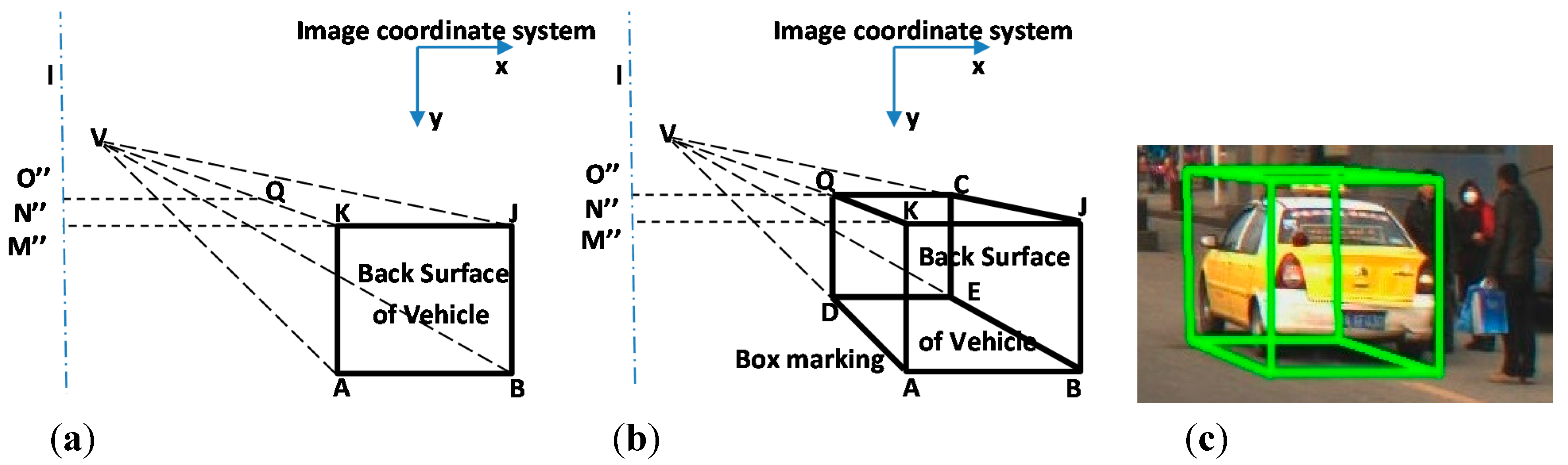
Figure 5. (a) and (b) depictions of the box marking drawing method. (c) Example of box marking in an image. The principal point $\text{O″}$ is the center point of the image, and the black rectangle KJAB is the vehicle back surface in the image plane, which are detected by the classifier described in Section 2.1. Point V is the vanishing point in the image. Line l is the perpendicular bisector of the image passing through principal point $\text{O″}$. Line K$\text{M″}$ is parallel to the x axis of the image and $\text{M″}$ is the intersection point on l. Line $\text{N″}$Q intersects lines VK and VJ at points Q and C, respectively. $\text{N″}$Q is parallel with $\text{M″}$K. Line QD intersects line VA at point D, and line DE intersects line VB at point E. Line QC and DE are parallel to the x axis and QD is parallel to the y axis of the image.

Figure 5. (a) and (b) depictions of the box marking drawing method. (c) Example of box marking in an image. The principal point $\text{O″}$ is the center point of the image, and the black rectangle KJAB is the vehicle back surface in the image plane, which are detected by the classifier described in Section 2.1. Point V is the vanishing point in the image. Line l is the perpendicular bisector of the image passing through principal point $\text{O″}$. Line K$\text{M″}$ is parallel to the x axis of the image and $\text{M″}$ is the intersection point on l. Line $\text{N″}$Q intersects lines VK and VJ at points Q and C, respectively. $\text{N″}$Q is parallel with $\text{M″}$K. Line QD intersects line VA at point D, and line DE intersects line VB at point E. Line QC and DE are parallel to the x axis and QD is parallel to the y axis of the image.

With the computed length of $\text{M″N″}$, the position of point $\text{N″}$ is known, then point C, D, and E can be located with the rules described in Figure 5. Thereafter, the black bolded-line region QCJBAD on Figure 5b can be determined. Based on the shape of the black bolded-line region, we defined it as the “box marking”. The region surrounded by the box marking will contain the front, back, and side-surfaces of the vehicle generally. Therefore, according to the description below, the box markings of vehicle side-surfaces can be fixed by $\text{M″N″}$.

Detecting vehicle side-surfaces by the box marking method has the advantage of having a fast speed and reliable results, but it relies on parameters H, f, and $\text{θ}$. These parameters can only be estimated crudely on driving recorders. Therefore, the above method can only locate the approximate position of the vehicle side surface. However, it is adequate for the method to reach the goal of eliminating features on the Mask.

2.3. Guardrail Detection

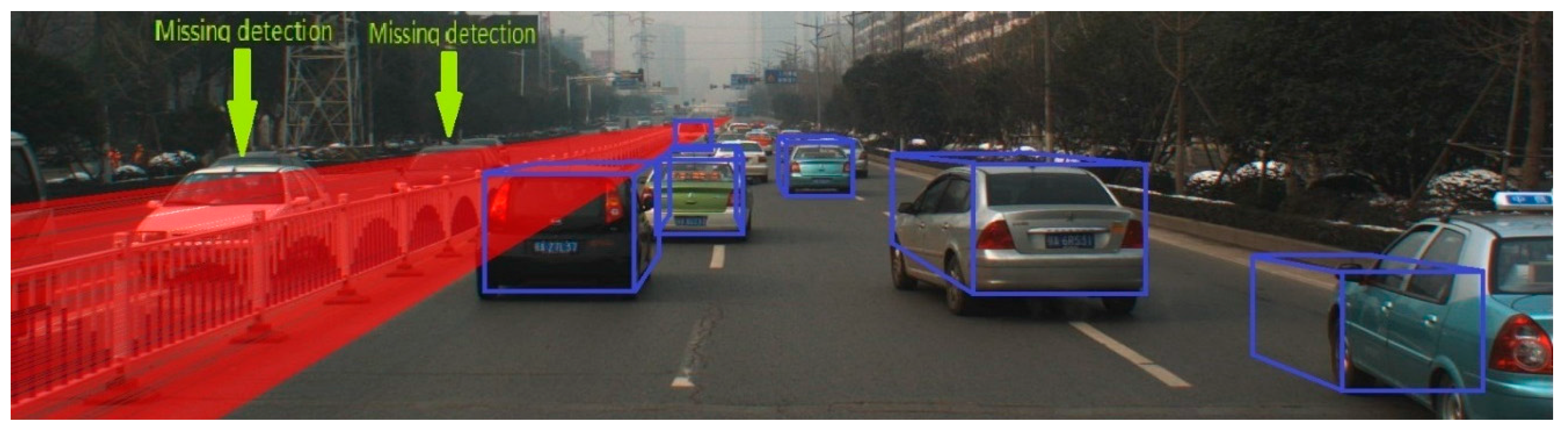
The guardrail is an isolation strip mounted on the center line of the road to separate vehicles running in opposite directions. It also can avoid pedestrian arbitrarily crossing the road. The photos of guardrail are shown in Figure 6d and Figure 7c. There are two reasons for detecting and removing the guardrail regions. The main reason is that, due to the repeating patterns of guardrails, they always contribute to poor matches. Furthermore, the views of vehicles moving on the other side of the guardrail are always blocked by the guardrails. This shielding makes vehicles undetectable by the vehicle classifiers. Therefore, in order to detect the blocked-vehicle regions, it was necessary to locate the guardrail regions. The blocked-vehicle regions detection method, which is described in Section 2.4, is based on the guardrail detection method described below.

The guardrail regions are detected based on a specially-designed guardrail-classifier. Except for changes in the training parameters, the guardrail-classifier training process is similar to the vehicle training method, which is described in Section 2.1. In order to detect an entire region of guardrails, a special guardrail-classifier was trained based on OpenCV Object Detection Lib [17] with a nearly 0% missing object rate. The price of a low missing rate, however, inevitably is an increase in the false detection rate, which means that the classifier could detect thousands of results that included not only the guardrails but also some background. In the training process, two parameters, the Stages-Number and the desired Min-Hit-Rate of each stage, were decreased. One parameter, the MinNeighbor [17] (a parameter specifying how many neighbors each candidate rectangle should have to retain it), was set to 0 during the detecting process.

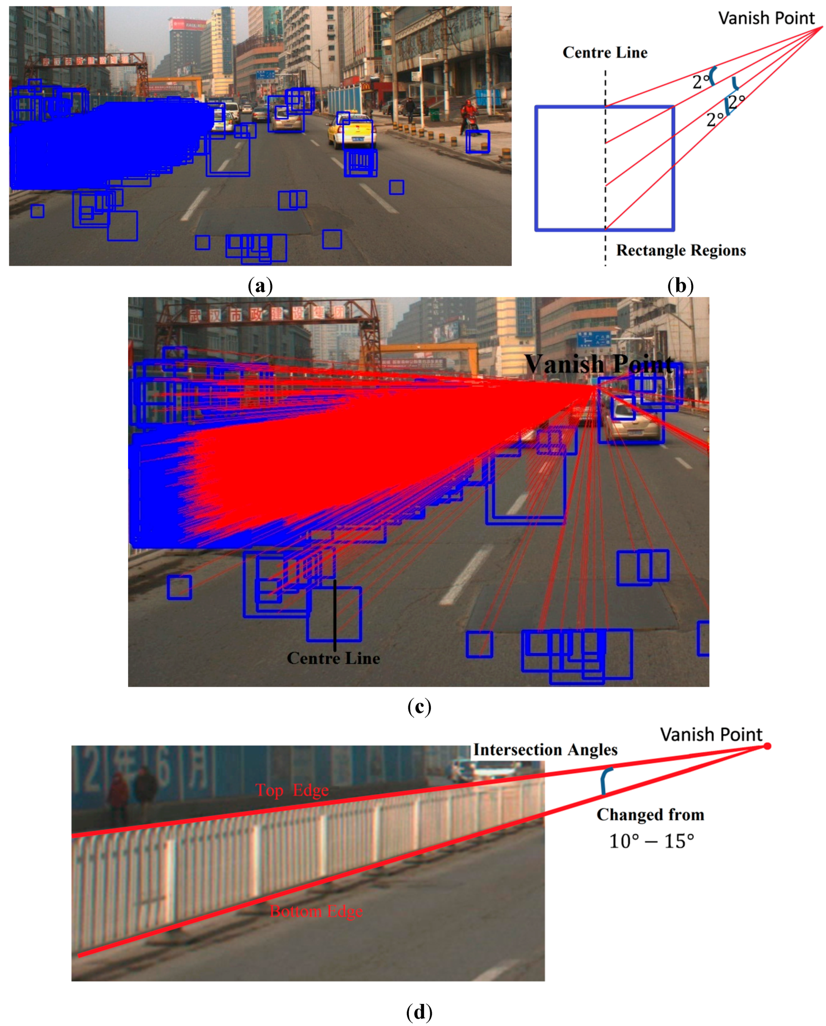
The special-designed guardrail classifier detection results are shown in Figure 6a as blue rectangles, and many of them are not guardrails. This is a side effect of guaranteeing a low missing object rate, but uses of the statistical analysis method can ensure that these false detections cannot influence the confirmation of the actual guardrail regions in further steps. The vanishing point was fixed by the [19,20] method, wherein a vanishing point is considered a point in the picture plane that is the intersection of a set of parallel lines in space on the picture plane. The lines are drawn from the vanishing point to each centre line of the rectangular regions at an interval of $2°$. This drawing approach is shown in Figure 6b, and the drawing results are shown in Figure 6c with red lines. Since the heights of the guardrails were fixed and the models in the driving recorder were changed within a certain range, the intersection angles between the guardrail top and bottom edges on the image often changed from $10°$ to $15°$ as a general rule. An example of the intersection angles is shown in Figure 6d.

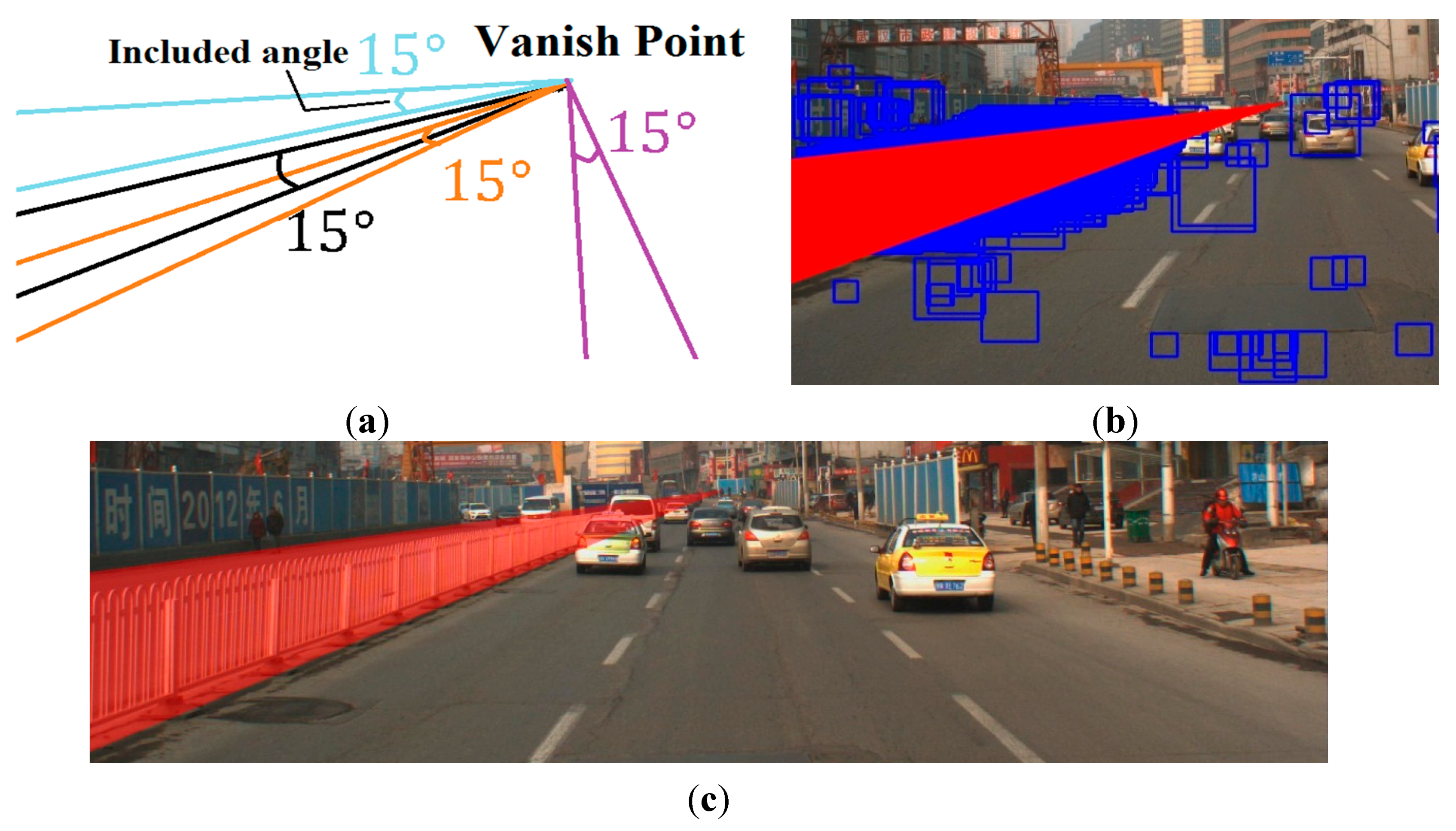
Based on the red lines drawn results, we made a triangle region which included an angle of $15°$ and a fixed vertex (the vanishing point). The threshold of $15°$ was the maximum potential intersection angle between the top and bottom edges of the guardrail. Then, we shifted the triangle region between $0°\text{ and }360°$ like Figure 7a. During the shift, the number of red lines included in every triangle region was counted. Then, we considered the triangle region that had the largest line numbers as the guardrail region. Figure 7b shows the position of the triangle region that had the largest line numbers, and Figure 7c shows the final detection results of the guardrail.

Figure 6. Guardrails detection process. (a) Detection results of a specially-designed guardrail-classifier which could detect thousands of results, including not only correct guardrails but many wrong detection regions as well. (b) Example of how to draw the red lines from the vanishing point to the detection regions. (c) Results of red lines drawn from the vanishing point to each centre line of the rectangle regions at an interval of $2°$. An example of a rectangle region’s centre line is shown in the bottom left corner of the (c); and (d) is an example of an intersection angle between the top and bottom edges of the guardrail.

Figure 6. Guardrails detection process. (a) Detection results of a specially-designed guardrail-classifier which could detect thousands of results, including not only correct guardrails but many wrong detection regions as well. (b) Example of how to draw the red lines from the vanishing point to the detection regions. (c) Results of red lines drawn from the vanishing point to each centre line of the rectangle regions at an interval of $2°$. An example of a rectangle region’s centre line is shown in the bottom left corner of the (c); and (d) is an example of an intersection angle between the top and bottom edges of the guardrail.

Figure 7. Guardrail location method. (a) Example of four triangle regions which included the angle of $15°$ and the fixed vertex (the vanishing point). (b) Triangle region that had the largest line numbers. (c) Final detection results of guardrail location method.

Figure 7. Guardrail location method. (a) Example of four triangle regions which included the angle of $15°$ and the fixed vertex (the vanishing point). (b) Triangle region that had the largest line numbers. (c) Final detection results of guardrail location method.

2.4. Blocked Vehicle Regions Detection

Sometimes, the vehicles that are moving in opposite direction can be blocked by guardrails, which results in the vehicle image overlapping with the guardrail partially. These occlusions make the vehicles undetectable by the front surface classifiers that were trained as described in Section 2.1. In this case, in order to detect blocked-vehicle regions, we increased the threshold of the intersection angle to broaden the guardrail region in order for the blocked vehicles to be included. In Figure 8, the blue box markings show the vehicle detection results based on the methods described in Section 2.1 and Section 2.2. Two vehicles are missing from the detection, which are indicated by the yellow arrows. The red triangle region is the broadened guardrail region with a $20°$ intersection angle. The missing detections are included by the broadened guardrail regions, which are shown in Figure 8.

Figure 8. Blocked vehicles detection method (guardrail region broadening method). Two vehicles running in opposite directions are missed detection by the vehicle classifier, which are indicated by the yellow arrows. These missed detection vehicle regions are included in the broadened guardrail regions, which are shown as the red region.

Figure 8. Blocked vehicles detection method (guardrail region broadening method). Two vehicles running in opposite directions are missed detection by the vehicle classifier, which are indicated by the yellow arrows. These missed detection vehicle regions are included in the broadened guardrail regions, which are shown as the red region.

2.5. Mask and Structure from Motion

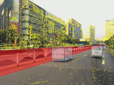
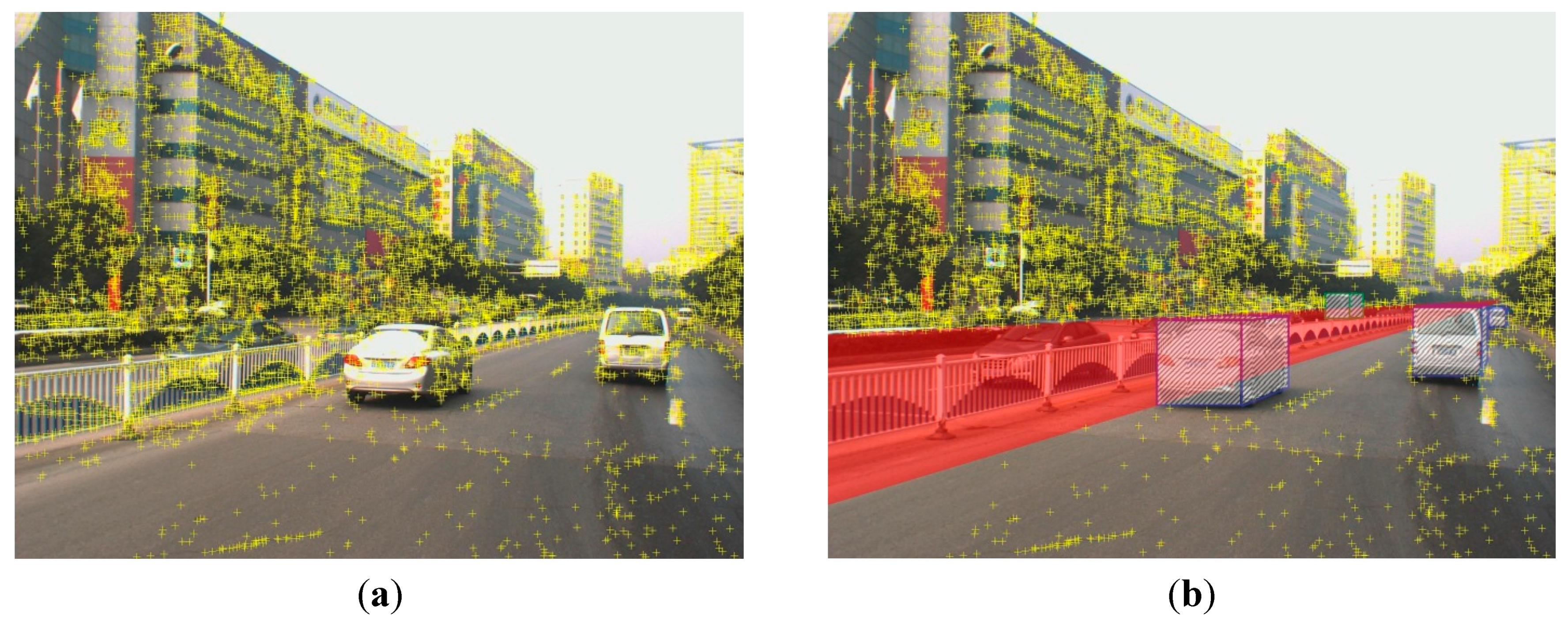
In the SIFT matching algorithm, detecting the feature points on the images is the first step, and the correspondences are then matched between the features. The coordinates of the features were compared with the location of the Mask regions in the image, and then the features located in the Mask were removed from the feature point sets. An example of our removing results is shown in Figure 9. The Mask was obtained by merging the regions detected in Section 2.1, Section 2.2, Section 2.3 and Section 2.4. After removing the SIFT feature points on the Mask, the remaining features were matched. Then, the QDEGSAC [21] algorithm was used to robustly estimate a fundamental matrix for each pair and the outliers were eliminated with a threshold of two pixels by the epipolar constraint [7,22]. The QDEGSAC algorithm is a robust model with a selection procedure that accounts for different types of camera motion and scene degeneracies. QDEGSAC is as robust as RANSAC [23] (the most common technique to deal with outliers in matches), even for (quasi-)degenerate data [21].

Figure 9. SIFT feature points removing results. (a) Original SIFT feature points set on image. (b) Mask results, which show the masked out features on the vehicle and guardrail regions.

Figure 9. SIFT feature points removing results. (a) Original SIFT feature points set on image. (b) Mask results, which show the masked out features on the vehicle and guardrail regions.

In a typical SfM reconstruction method, pairwise images are matched with the SIFT algorithm without any added process. Then, the inlier matches are determined by the epipolar constraint algorithm (similar to the QDEGSAC algorithm), and a sparse point cloud is reconstructed with the inliers by the SfM algorithm. However, in our method, during the pairwise matching process, the SIFT feature points on the vehicle and guardrail regions are masked out before matching. The remaining features are then matched by the SIFT algorithm. After the outliers were eliminated by the epipolar constraint algorithm, the SfM reconstruction process proceeds with the remaining matches.

Both in the typical method and our proposed method, the QDEGSAC algorithm was used as an epipolar constraint algorithm to select the inliers, and the SfM process was conducted in VisualSFM [24,25]. Visual SFM is a GUI application of the incremental SfM system. It runs very fast by exploiting multi-core acceleration. The features mask out process in our method is the only difference from the typical method.

3. Experiment

3.1. Test Data and Platform

A driving recorder is a camera mounted on the dashboard of a vehicle that can record images when the vehicle is moving. The SfM reconstruction method can accept various image sizes from different types of recorders. We used 311 images taken by five recorders on roundabout as testing data to demonstrate the improved results with our method. We chose images taken on roundabout at large intervals to increase the complexity of the testing data. The Storm Media Player was used to extract images from videos. We manually extracted images with the intervals which are described in Table 1. The characteristics of the testing data are described below:

• The testing images were taken by five recorders mounted on four vehicles, and the largest time interval between the two image sequences was nearly three years.
• A total of 125 images were extracted from videos recorded by driving recorders 1, 2, and 3.
• 186 images were recorded by recorders 4 and 5, which were mounted on the same vehicle with identical exposure intervals.
• Roundabout was crowded during the recording time so the survey vehicles changed their lanes and speeds when necessary to move with the traffic.
• The rest details of recorders and images are shown in Table 1.

Table 1. The characteristics of recorders and images.

Recorder NO	Sensor Type	Focus Style	Image Size	Image Extraction Intervals	Recording Date
1, 2, 3	Video	Zoom Lens	1920 × 1080	About 1 s	12/23/2014
4, 5	Camera	Fixed Focus	800 × 600	0.5 s	1/23/2012

Table 1. The characteristics of recorders and images.

Recorder NO	Sensor Type	Focus Style	Image Size	Image Extraction Intervals	Recording Date
1, 2, 3	Video	Zoom Lens	1920 × 1080	About 1 s	12/23/2014
4, 5	Camera	Fixed Focus	800 × 600	0.5 s	1/23/2012

We separated 311 images into sequences 1, 2, 3, 4, and 5 according to the recorder that recorded them. The results are shown in Table 2.

Table 2. The composition of three sets.

Set Number	Recorder Number	Image Number	Attribute
1	4, 5	186	Stereo images taken by two cameras mounted on the same vehicle with identical exposure intervals.
2	1, 2, 3, 4	218	The longest time interval between the two image sequences was nearly three years, and the images were two different sizes.
3	1, 2, 3, 4, 5	311	Three monocular and two stereo image sequences. The longest time interval between the two image sequences was nearly three years, and the images were two different sizes.

Table 2. The composition of three sets.

Set Number	Recorder Number	Image Number	Attribute
1	4, 5	186	Stereo images taken by two cameras mounted on the same vehicle with identical exposure intervals.
2	1, 2, 3, 4	218	The longest time interval between the two image sequences was nearly three years, and the images were two different sizes.
3	1, 2, 3, 4, 5	311	Three monocular and two stereo image sequences. The longest time interval between the two image sequences was nearly three years, and the images were two different sizes.

We conducted all the following experiments on a PC with an Intel Core i7-3770 3.4 GHz CPU (8cores), 4 GB RAM, and an AMD Radeon HD 7000 series GPU. The detection algorithm was implemented in a Visual C++ platform with the OpenCV 2.4.9 libraries. Training each vehicle classifier took nearly 75 h, and eight hours was required for training the guardrail classifier. Although training the classifier was a time-consuming process, the trained classifier could be used to detect vehicles at a fast speed after one-off training. The detection speed was affected by the number of targets. When running on the described PC, the average detecting time was 0.15 s for each classifier on a 1600 × 1200 pixel-sized image. In the following section, we compare the performance between the typical SfM reconstruction method and our method from three aspects: the precision of pairwise orientation, the recovered camera tracks, and the reconstructed point clouds, which are described in Section 3.2, Section 3.3 and Section 3.4, respectively.

3.2. Precision of Pairwise Orientation

In the SfM system, the accuracy of the reconstructed point clouds is determined by the quality of the correspondences. Hence, in this section, we evaluate and compare the matching results of the typical method and our method by the root-mean-square error (RMSE).

Based on the epipolar constraint, correspondences ${\text{p}}_{\text{i}}$, ${\text{p}}_{\text{i}}^{\text{′}}$ should be located on the corresponding epipolar line ${\text{ l}}_{\text{i}}$, ${\text{l}}_{\text{i}}^{\text{′}}$ respectively (The epipolar line can be computed with the algorithm proposed by D. Nister [26]). However ${\text{p}}_{\text{i}}^{\text{′}}$ may deviate from epipolar line ${\text{l}}_{\text{i}}^{\text{′}}$ due to orientation errors. Thereafter, the RMSE is able to evaluate the accuracy of the pairwise orientation with following equation.

$$\text{RMSE}=\sqrt{\frac{{\text{d}}_1^2+{\text{d}}_2^2+\cdots {\text{d}}_{\text{n}}^2}{\text{n}}}$$

(23)

${\text{d}}_{\text{i}}$ in Equation (23) is the distance between point ${\text{p}}_{\text{i}}^{\text{′}}$ and the epipolar line ${\text{l}}_{\text{i}}^{\text{′}}$. n is the number of matches. The pixel size of CCD was 0.0044 mm; therefore millimeter was used as the unit of RMSE.

The difference between the typical method and our method is that our method masked out the feature points on vehicles and guardrails before proceeding with matching. Then, in both the typical method and our method, the correspondences with ${\text{d}}_{\text{i}}$ greater than the threshold (two pixels) were eliminated by the QDEGSAC algorithm [21] before inputting into Equation (23).

In order to demonstrate the improvement and robustness of our method, 666 image pairs of diverse street scenes were chosen randomly using the above image set. The RMSE of the pairwise orientation results by the typical method and our method are shown in Figure 10.

In Figure 10, the RMSEs in our method were less than in the typical method in general. The abnormity in the image pairs (the RMSEs in our method were larger than the typical method) for which we offer the following analysis. We found that the abnormal pairs were usually shot at long-range distances (more than 200 m) with little overlap, leading ultimately to a decrease in the number of accurate matches. A large proportion of the outliers led to an orientation failure, which produced abnormal RMSE results. In general, however, it can be concluded from Figure 10 that the Mask effectively improved the matching accuracy.

Figure 10. RMSEs of each image. The X-axis represents the serial number of the image pairs and the Y-axis represents the RMSEs, which are shown as millimeters. The blue and red lines show the RMSEs of the typical method and our method, respectively. The correspondences in our method were matched after removing the SIFT features on the Mask, and then the outliers were eliminated by the epipolar constraint (QDEGSAC) method. In the typical method, the correspondences were filtered only by the epipolar constraint (QDEGSAC) method.

Figure 10. RMSEs of each image. The X-axis represents the serial number of the image pairs and the Y-axis represents the RMSEs, which are shown as millimeters. The blue and red lines show the RMSEs of the typical method and our method, respectively. The correspondences in our method were matched after removing the SIFT features on the Mask, and then the outliers were eliminated by the epipolar constraint (QDEGSAC) method. In the typical method, the correspondences were filtered only by the epipolar constraint (QDEGSAC) method.

3.3. Camera Poses Recovering Results

Figure 11 is an explanation of the reconstructed camera-pose-triangle in the following figures. The colored triangles represent the position of the recovered image/camera. Figure 12, Figure 13 and Figure 14 shows the camera pose reconstruction results of three sets. The details and compositions of each set were described in Table 2. The difference between the typical method and our method is that the feature points on the Mask are removed before matching in our method. Since motor vehicles can only run in a smooth track, we were able to distinguish an unordered track as false reconstruction results easily.

Figure 11. Explanation of the reconstructed camera-pose-triangle and driving tracks. (a) Colored triangle represents the position of the recovered image and the camera projective center. The size of the triangle is followed by the size of the image data. (b) Red line represents the recovered vehicle driving tracks that carried recorder 1. The colored triangles are the reconstructed results that represent the position of the images taken by recorder 1.

Figure 11. Explanation of the reconstructed camera-pose-triangle and driving tracks. (a) Colored triangle represents the position of the recovered image and the camera projective center. The size of the triangle is followed by the size of the image data. (b) Red line represents the recovered vehicle driving tracks that carried recorder 1. The colored triangles are the reconstructed results that represent the position of the images taken by recorder 1.

Figure 12. The recovered image positions of Set 1. These images were taken by recorders 4 and 5, which had the same exposure interval and were mounted on one vehicle. (a) and (b) are the recovered results from the same data with different methods. (a) depicts the reconstruction by the typical SfM method. The recovered images in the red rectangle of (a) are unordered obviously. (b) depicts the reconstruction by our method (features on vehicles and guardrails were masked out before matching and reconstruction). (c) is not a georeferenced result. We manually scaled the results of (b) and put it on the Google satellite map to help readers visualize the rough locations of the image sequences on roundabout.

Figure 12. The recovered image positions of Set 1. These images were taken by recorders 4 and 5, which had the same exposure interval and were mounted on one vehicle. (a) and (b) are the recovered results from the same data with different methods. (a) depicts the reconstruction by the typical SfM method. The recovered images in the red rectangle of (a) are unordered obviously. (b) depicts the reconstruction by our method (features on vehicles and guardrails were masked out before matching and reconstruction). (c) is not a georeferenced result. We manually scaled the results of (b) and put it on the Google satellite map to help readers visualize the rough locations of the image sequences on roundabout.

Figure 13. The recovered image positions of Set 2. These images were taken by recorders 1, 2, 3, and 4 mounted on their respective vehicles. (a) Reconstruction by the typical SfM method. The recovered disordered images in the red rectangles of (a) were recorded by recorder 4. (b) is not a georeferenced result. We manually scaled the results of (a) and put it on the Google satellite map. Based on the enlargement in (a) and the visualized rough location in (b), it can be seen that they were reconstructed in the wrong place. (c) Reconstruction by our method (features on vehicles and guardrails were masked out before matching and reconstruction). The recovered triangles of recorder 4 are smaller than the others because the sizes of the images taken by recorder 4 were smaller than those of the other recorders, which is reflected in (c) by the different reconstructed sizes of the triangles. (a) and (c) are the recovered results from the same data using different methods.

Figure 13. The recovered image positions of Set 2. These images were taken by recorders 1, 2, 3, and 4 mounted on their respective vehicles. (a) Reconstruction by the typical SfM method. The recovered disordered images in the red rectangles of (a) were recorded by recorder 4. (b) is not a georeferenced result. We manually scaled the results of (a) and put it on the Google satellite map. Based on the enlargement in (a) and the visualized rough location in (b), it can be seen that they were reconstructed in the wrong place. (c) Reconstruction by our method (features on vehicles and guardrails were masked out before matching and reconstruction). The recovered triangles of recorder 4 are smaller than the others because the sizes of the images taken by recorder 4 were smaller than those of the other recorders, which is reflected in (c) by the different reconstructed sizes of the triangles. (a) and (c) are the recovered results from the same data using different methods.

Figure 14. The recovered image positions of Set 3. These images were taken by recorders 1–5. (a) and (b) are the recovered results from the same data with different methods; (a) was reconstructed by the typical SfM method and (b) was reconstructed by our method (features on vehicles and guardrails were masked out before matching and reconstruction). The images in red rectangles in (a) were recovered in chaos. (c) is not a georeferenced result. We manually scaled the recovery results of our method and put it on the Google satellite map to help readers visualize the rough locations of the image sequences on roundabout.

Figure 14. The recovered image positions of Set 3. These images were taken by recorders 1–5. (a) and (b) are the recovered results from the same data with different methods; (a) was reconstructed by the typical SfM method and (b) was reconstructed by our method (features on vehicles and guardrails were masked out before matching and reconstruction). The images in red rectangles in (a) were recovered in chaos. (c) is not a georeferenced result. We manually scaled the recovery results of our method and put it on the Google satellite map to help readers visualize the rough locations of the image sequences on roundabout.

The contrast experiment results show that the recovery performance of our method was better than the typical SfM method in each set. In contrast, the typical method was unable to recover an entire track of cameras in each set while the camera poses were recovered smoothly with our method.

We can infer from the above results that the typical method sometimes returns unreliable recovery results, especially for multi-sensors’ data.

3.4. Sparse 3D Point Clouds Reconstruction Results

Sparse 3D point clouds can be reconstructed by the SfM algorithm with VisualSFM and Photosynth [27]. Photosynth is a powerful set of tools designed by Microsoft’s Live Labs. It builds on a structure-from-motion system for unordered image collections, which is based on the Photo Tourism [10,11] research conducted by the University of Washington and Microsoft Research [27]. The structure from motion module in Photo Tourism comes from Bundler [10,11], which is one of the most developed SfM systems. As a useful tool, Bundler has been widely used in many point clouds reconstruction researches. This is the main reason why we chose the Photosynth as the contrast experiment tool. Furthermore, the high-level automation and widely using of Photosynth can also explain our choice. The reason why we chose VisualSFM is that VisualSFM is a powerful SfM tool; it has a flexible interface and stable performance. It is also frequently used in 3D reconstruction researches.

From the data all combined in Table 2, Set 3 is sufficient enough to cover the results from Set 1 and 2. Besides, the data collected by Recorder 1–5 in different image sizes had been lasting for as long as three years. Thus, Set 3 is able to contain various data from different cameras, which means that it is more representative than using Set 1 and 2 to evaluate the performance of reconstruction methods. Therefore, the following experiments were used VisualSFM and Photosynth based on the 311 images in Set 3. Figure 15 shows the model of main target buildings we aimed to reconstruct. Figure 16 and Figure 17 show the side and vertical views of the results of the three methods, respectively.

The results in Figure 16 and Figure 17 indicate that even the developed 3D reconstruction tool Photosynth is not capable of dealing with driving recorder data directly. However, the camera tracks and sparse point clouds were reconstructed successfully using the mask out correspondences as inputs to run SfM.

Figure 15. Main targets in the sparse point clouds reconstruction process. The two building models in (a) and (b) with red and yellow marks are the main reconstruction targets. (a) and (b) are the side and oblique bird’s-eye view of two buildings from Google Earth, respectively.

Figure 15. Main targets in the sparse point clouds reconstruction process. The two building models in (a) and (b) with red and yellow marks are the main reconstruction targets. (a) and (b) are the side and oblique bird’s-eye view of two buildings from Google Earth, respectively.

Figure 16. Side view of main target reconstruction results with sparse point clouds. Each result was reconstructed with the same data of 311 images in Set 3. (a) Sparse point clouds reconstructed by Photosynth without any added processing. The building on the left marked in red was repetitively reconstructed. (b) Sparse point clouds reconstructed by VisualSFM with the typical method. The building on the right could not be reconstructed and should be positioned inside the yellow box. (c) Sparse point clouds reconstructed by VisualSFM with our method. The details of the differences between the typical method and our method are described in Section 2.5 but can be summarized by saying that our method removed the features on the Mask and matched the remaining feature points before reconstruction.

Figure 16. Side view of main target reconstruction results with sparse point clouds. Each result was reconstructed with the same data of 311 images in Set 3. (a) Sparse point clouds reconstructed by Photosynth without any added processing. The building on the left marked in red was repetitively reconstructed. (b) Sparse point clouds reconstructed by VisualSFM with the typical method. The building on the right could not be reconstructed and should be positioned inside the yellow box. (c) Sparse point clouds reconstructed by VisualSFM with our method. The details of the differences between the typical method and our method are described in Section 2.5 but can be summarized by saying that our method removed the features on the Mask and matched the remaining feature points before reconstruction.

Figure 17. Vertical view of main target reconstruction results with sparse point clouds. Each result was reconstructed by same data of 311 images in Set 3. (a) Sparse point clouds reconstructed by Photosynth without any added processing. The result is chaos. Expecting the repetition we experienced as shown in Figure 16, it can be clearly seen that not only was the left building repeatedly reconstructed, but the right building was as well. The repetitive reconstructions of the buildings are marked in red for the left building and the right building is in yellow. (b) Sparse point clouds reconstructed by VisualSFM with the typical method. The right building was missed which should be reconstructed inside the yellow mark. (c) Sparse point clouds reconstructed by VisualSFM with our method. The details between the typical method and our method are described in Section 2.5, which can be summarized by saying that we removed the features on the Mask and matched the remaining feature points before reconstruction. (d) shows a more intuitive result. It is not a georeferenced result. We manually scaled the sparse point clouds of our method and put it on the Google satellite map, which can help readers visualize the high level of overlapping between the point clouds and the map, the rough relative positions of the two buildings, and the position of recovered images in roundabout.

Figure 17. Vertical view of main target reconstruction results with sparse point clouds. Each result was reconstructed by same data of 311 images in Set 3. (a) Sparse point clouds reconstructed by Photosynth without any added processing. The result is chaos. Expecting the repetition we experienced as shown in Figure 16, it can be clearly seen that not only was the left building repeatedly reconstructed, but the right building was as well. The repetitive reconstructions of the buildings are marked in red for the left building and the right building is in yellow. (b) Sparse point clouds reconstructed by VisualSFM with the typical method. The right building was missed which should be reconstructed inside the yellow mark. (c) Sparse point clouds reconstructed by VisualSFM with our method. The details between the typical method and our method are described in Section 2.5, which can be summarized by saying that we removed the features on the Mask and matched the remaining feature points before reconstruction. (d) shows a more intuitive result. It is not a georeferenced result. We manually scaled the sparse point clouds of our method and put it on the Google satellite map, which can help readers visualize the high level of overlapping between the point clouds and the map, the rough relative positions of the two buildings, and the position of recovered images in roundabout.

Since the images recorded by a driving recorder have no GPS information, there is no other data available that can provide the absolute coordinates of the reconstructed point cloud. So in order to quantify the sparse point clouds, the plane fitting method is proposed below.

Figure 18. The vertical view of the two planes. (a) shows the sparse point clouds reconstructed by VisualSFM with our method. The Plane 1 and 2 are target planes we fitted. (b) shows the position of the target wall-planes in Google Map. (c) shows the Plane 1 and 2 in street view. (d) Example of plane fitted result in vertical view. The red line respects the vertical view of the plane fitted by wall points, and the blue lines are examples of the distances between the plane and points.

Figure 18. The vertical view of the two planes. (a) shows the sparse point clouds reconstructed by VisualSFM with our method. The Plane 1 and 2 are target planes we fitted. (b) shows the position of the target wall-planes in Google Map. (c) shows the Plane 1 and 2 in street view. (d) Example of plane fitted result in vertical view. The red line respects the vertical view of the plane fitted by wall points, and the blue lines are examples of the distances between the plane and points.

As we know, the points on the same wall also should lie on the same plane in the point cloud. Based on that principle, the distance between the fitted plane and the reconstructed wall point can be used to confirm whether the reconstruction performed well. Planes 1 and 2 in Figure 18 are the planes we aimed to fit. We manually chose the reconstructed points belonging to the above walls to fit the Plane 1 and 2. The fitting method is based on the Equation (24), the Plane Equation. According to the Least Square method, the equation of each plane was computed with the coordinates of points.

$$\text{Ax}+\text{By}+\text{Cz}+\text{D}=0$$

(24)

The x, y and z are coordinates of points; they are in relative coordinate system. In addition, the A, B, C and D are plane parameters that should be calculated by the Least Square method.

Based on the computed plane, the distances between the fitted plane and each wall point were then calculated. The maximum distance, minimum distance and RMSE of distance in the typical method and our method are shown in Table 3 below. Since there is no GPS information or other data available that can provide the geographical reference, the results are compared in the relative coordinates.

Table 3. The fitting results between the typical method and the proposed method. The results are in relative coordinates system.

Plane NO.	Typical Method			Proposed Method
	RMSE	Maximum	Minimum	RMSE	Maximum	Minimum
1	0.0047	0.0170	$4.420\times {10}^{-6}$	0.0031	0.0142	$1.887\times {10}^{-6}$
2	0.0171	0.0994	$2.133\times {10}^{-5}$	0.0095	0.0705	$1.220\times {10}^{-5}$

Table 3. The fitting results between the typical method and the proposed method. The results are in relative coordinates system.

Plane NO.	Typical Method			Proposed Method
	RMSE	Maximum	Minimum	RMSE	Maximum	Minimum
1	0.0047	0.0170	$4.420\times {10}^{-6}$	0.0031	0.0142	$1.887\times {10}^{-6}$
2	0.0171	0.0994	$2.133\times {10}^{-5}$	0.0095	0.0705	$1.220\times {10}^{-5}$

Table 3 shows the RMSE decreased by 30–40 percentages in proposed method that indicated that the accuracies of reconstructed planes are improved in our method. Based on the above results, it is clearly seen that masking out the features from vehicles and guardrails can improve the reconstruction results. We also found our method to be robust enough for driving recorder data sets composed of different-sized images having nearly three years recovered intervals.

4. Discussion

This paper focused on sparse point cloud reconstruction with the features removed on the Mask. The Mask is the region where features should be eliminated before matching in order to avoid generating outliers. The Mask was first detected from the unstructured and uncontrolled driving recorder data automatically. Then, the feature points on Mask were eliminated before feature matching. Finally a SfM procedure with the remaining correspondences was performed.

The advantage of using driving recorder data is that a driving recorder can acquire city-scale street scenes less expensively. This low-cost data in larger quantities can support reconstructing and updating sparse street point clouds in shorter update periods of time. The improved reconstruction results are shown in Section 3 from three aspects: the precision of pairwise orientation, the recovered camera tracks, and the reconstructed point clouds. In the contrast experiment presented in Section 3.4, the right building was missing in the results of the typical SfM process [24,25] (shown in Figure 16b and Figure 17b), which was caused by the disordered camera poses’ recovered results shown in Section 3.3, Figure 14a. We found that these disordered images generally were crowded with a large number of moving vehicles, which led to poor matches. It was also proven that the commercial software Photosynth [27], which is based on the Photo Tourism [10,11] technology, was not able to provide good performance with the driving recorder data. The reconstructed points indicate obvious chaos, and the buildings were repeatedly reconstructed incorrectly. The disordered point clouds were shown in Figure 16a and Figure 17a in Section 3.4. The overall quality of the point clouds is reflected in the comparison between the results shown in Figure 16 and Figure 17. Furthermore, there were no other data to provide the absolute coordinates of the reconstructed point clouds so we qualified the point clouds with the plane fitting results in Table 3 and the overlap between the point clouds and Google satellite map in Figure 17d. In Figure 17d, the points are fitted with the map generally, which reflects the high level of overlapping between the point clouds and the map. The plane fitting results in Table 3 indicate that the reconstruction accuracy of the proposed method is higher than the typical method based on the decreased average distance between the fitted plane and the points.

The features mask method is based on one important factor: the SIFT algorithm can generate a large number of features that densely cover the image over the full range of scales and locations [12]. Approximately 1000–2000 correspondences can be matched with the SIFT algorithm on one pair of driving recorder data which cover more than 70% of the overlap. Generalized from ample experiments, the matching points on the Mask took a 21% proportion of the total matching points. Therefore, although the bad points on the Mask were removed, the remaining correspondences were adequate to recover the camera poses and point clouds of the street scene.

Although redundant data theoretically can produce better reconstruction results, a large number of data would adversely affect efficiency due to the fact that full pairwise matching takes $\text{O}\left(n^2\right)$ time for n input images, which is why the Mask method is used to improve the reconstruction results instead of simply increasing the data sets. Detecting and removing the Mask regions with our methods proposed in this paper only takes a few seconds in each image. The Mask results show that it can improve the quality of the matches, which may lead to a higher level of efficiency than the redundancy method.

The proposed reconstruction method is effective when the solution is scaled up. It also relies on the scalability of the SfM method. One of the most difficult problems of SfM is that it is time-intensive. There have been many relative research efforts aimed at shortening the reconstruction time, such as the vocabulary tree [28] and the Building Rome on a cloudless day [8]. The SfM method has been used to reconstruct an entire city with Internet photos. The paper aims to shorten the reconstruction time by the parallelism and throughput [8]. Our method can be a supplement to these methods, which means that, with the help of vocabulary tree and parallel computing, it can reconstruct an entire city with ample driving recorder images. Then, this method may replace mobile mapping technologies in some applications like updating 3D street data that have been georeferenced or reconstructing city-scale point clouds in relative coordinate systems.

The proposed method can reconstruct street scenes robustly with different-sized images, taken on different roads or with different lighting conditions; however, the images taken at night always contribute less to the reconstruction process. Obviously, the matches decrease in night images since the difference in building textures between day and night images are influenced by the city lighting. Similarly, lower quality will lead to fewer correspondences, which may not cause fatal mistakes to reconstruction but will increase the time consumed. Therefore if we ignore the efficiency and the data set is big enough, there is no strict requirement for the quality of image data.

The proposed method has one limitation. Since the driving recorder is always mounted to record traffic rather than buildings, the taller sections of nearby building cannot be recorded, thereby generating sparse reconstructed points for them. In general, three main innovations are presented in this paper:

• We proposed a street scene reconstruction method from driving recorder data. This new method makes full use of the massive amount of data produced by driving recorders with shorter update time, which can reduce the costs of recovering 3D sparse point clouds compared to mobile mapping equipment carrying stable GPS/INS systems. In order to improve the recovery accuracy, we analyzed and summarized the distribution regularities of the outliers from the SIFT matching results through ample experiments.
• Our work differs from the typical SfM approaches, in that, we eliminate the feature points on the Mask before matching is undertaken. We also proved through experiments that the relative orientation results and reconstruction results improved after removing the feature points on the Mask.
• We designed guardrail and vehicle side region detecting methods based on the characteristics of the driving recorder data. The detection methods are based on the trained Haar-like-feature cascade classifiers, the position of the vanishing point, and some camera parameters.

5. Conclusions

This paper proposed a method to reconstruct street scenes with data from driving recorders, which are widely used in private and public vehicles. This low-cost method will be beneficial to reducing the cost and shortening the update time required for street scene reconstruction. However, using the unprocessed driving recorder data was found to contribute to the failure of reconstruction due to the large number of inevitable outliers on moving vehicles and guardrails with repeating patterns.

Based on our analysis from numerous SIFT matching results, we then proposed a method for removing the features on vehicle and guardrail regions, which is called the Mask in this paper. In order to remove the feature points on the Mask, an automatic detecting method was designed. As shown in Section 3, the proposed method improved the results in three areas: the precision of the pairwise orientation, the recovery performance of the camera poses, and the reconstruction results of the point clouds.

Our work differs from typical SfM approaches in that we remove the features on the Mask in order to improve the accuracy of the street scene reconstruction results from driving recorder data. The proposed method can be improved in the following areas, which will be the subjects of future research.

• Reconstructing robust side surfaces in the vehicle detection method without camera parameters.
• Extracting the most appropriate images from driving recorder videos.
• Reducing the number of images in the time-consuming matching step with a reasonable strategy.
• Increasing the density of reconstructed point clouds.
• Detecting the blocked vehicles with more accuracy in a region.

References

1. Habib, A.; Pullivelli, A.; Mitishita, E.; Ghanma, M.; Kim, E. Stability analysis of low-cost digital cameras for aerial mapping using different georeferencing techniques. Photogramm. Rec. 2006, 21, 29–43. [Google Scholar] [CrossRef]
2. Zhang, Y.; Zhang, Z.; Zhang, J.; Wu, J. 3D building modelling with digital map, LiDAR data and video image sequences. Photogramm. Rec. 2005, 20, 285–302. [Google Scholar] [CrossRef]
3. Xiao, J.; Fang, T.; Zhao, P.; Lhuillier, M.; Quan, L. Image-based street-side city modeling. Acm Trans. Graph. 2009, 28. [Google Scholar] [CrossRef]
4. Cornelis, N.; Leibe, B.; Cornelis, K.; van Gool, L. 3D urban scene modeling integrating recognition and reconstruction. Int. J. Comput. Vis. 2008, 78, 121–141. [Google Scholar] [CrossRef]
5. Aijazi, A.; Checchin, P.; Trassoudaine, L. Automatic removal of imperfections and change detection for accurate 3D urban cartography by classification and incremental updating. Remote Sens. 2013, 5, 3701–3728. [Google Scholar] [CrossRef]
6. Williams, K.; Olsen, M.; Roe, G.; Glennie, C. Synthesis of transportation applications of mobile LiDAR. Remote Sens. 2013, 5, 4652–4692. [Google Scholar] [CrossRef]
7. Hartley, R.; Zisserman, A. Multiple View Geometry in Computer Vision, 2nd ed.; Cambridge University Press: New York, NY, USA, 2003. [Google Scholar]
8. Frahm, J.; Lazebnik, S.; Fite-Georgel, P.; Gallup, D.; Johnson, T.; Raguram, W.C.; Jen, Y.; Dunn, E.; Clipp, B. Building Rome on a cloudless day. In Proceeding of the 2010 Europe Conference on Computer Vision (ECCV), Crete, Greece, 5–11 September 2010; Volume 6314, pp. 368–381.
9. Raguram, R.; Wu, C.; Frahm, J.; Lazebnik, S. Modeling and recognition of landmark image collections using iconic scene graphs. Int. J. Comput. Vis. 2011, 95, 213–239. [Google Scholar] [CrossRef]
10. Snavely, N.; Seitz, S.M.; Szeliski, R. Photo tourism: Exploring photo collections in 3D. ACM Trans. Graph. 2006, 25. [Google Scholar] [CrossRef]
11. Snavely, N.; Seitz, S.M.; Szeliski, R. Modeling the world from internet photo collections. Int. J. Comput. Vis. 2008, 80, 189–210. [Google Scholar] [CrossRef]
12. Lowe, D.G. Distinctive image features from scale-invariant keypoints. Int. J. Comput. Vis. 2004, 60, 91–110. [Google Scholar] [CrossRef]
13. Viola, P.; Jones, M. Rapid object detection using a boosted cascade of simple features. In Proceedings of the 2001 IEEE Computer Society Conference on Computer Vision and Pattern Recognition, Kauai, HI, USA, 8–14 December 2001; Volume 1, pp. 511–518.
14. Lienhart, R.; Maydt, J. An extended set of haar-like features for rapid object detection. In Proceedings of the 2002 International Conference on Image Processing, New York, NY, USA, 22–25 September 2002; pp. 900–903.
15. Schapire, R.E.; Singer, Y. Improved boosting algorithms using confidence-rated predictions. Mach. Learn. 1999, 37, 297–336. [Google Scholar] [CrossRef]
16. Ponsa, D.; Lopez, A.; Lumbreras, F.; Serrat, J.; Graf, T. 3D vehicle sensor based on monocular vision. In Proceedings of the 2005 IEEE Intelligent Transportation Systems, Vienna, Austria, 13–16 September 2005; pp. 1096–1101.
17. OpencvTeam OpenCV 2.4.9.0 Documentation. Available online: http://docs.opencv.org/modules/objdetect/doc/cascade_classification.html (accessed on 18 October 2014).
18. Jiang, J.L.; Loe, K.F. S-AdaBoost and pattern detection in complex environment. In Proceedings of the 2003 IEEE Computer Society Conference on Computer Vision and Pattern Recognition (CVPR’03), Los Alamitos, CA, USA, 18–20 June 2003; pp. 413–418.
19. Kutulakos, K.N.; Sinha, S.N.; Steedly, D.; Szeliski, R. A multi-stage linear approach to structure from motion. In Trends and Topics in Computer Vision; Kutulakos, K.N., Ed.; Springer: Berlin, Germany, 2012; pp. 267–281. [Google Scholar]
20. Moghadam, P.; Starzyk, J.A.; Wijesoma, W.S. Fast vanishing-point detection in unstructured environments. IEEE Trans. Image Process. 2012, 21, 425–430. [Google Scholar] [CrossRef] [PubMed]
21. Frahm, J.M.; Pollefeys, M. RANSAC for (Quasi-) degenerate data (QDEGSAC). In Proceedings of the 2006 IEEE Computer Society Conference on Computer Vision and Pattern Recognition (CVPR′06), New York, NY, USA, 17–22 June 2006; Volume 1, pp. 453–460.
22. Torr, P.; Zisserman, A. Robust computation and parametrization of multiple view relations. In Proceedings of the Sixth International Conference on Computer Vision, Bombay, India, 4–7 January 1998; pp. 727–732.
23. Fischler, M.A.; Bolles, R.C. Random sample consensus: A paradigm for model fitting with applications to image analysis and automated cartography. Commun. ACM 1981, 24, 381–395. [Google Scholar] [CrossRef]
24. Wu, C. VisualSFM: A Visual Structure from Motion System. Available online: http://ccwu.me/vsfm/ (accessed on 8 October 2014).
25. Wu, C. Towards linear-time incremental structure from motion. In Proceedings of the 2013 International Conference on 3D Vision IEEE, Seattle, WA, USA, 29 June–1 July 2013; pp. 127–134.
26. Nister, D. An efficient solution to the five-point relative pose problem. IEEE Trans. Pattern Anal. Mach. Intell. 2004, 26, 756–777. [Google Scholar] [CrossRef] [PubMed]
27. Microsoft Corporation. Photosynth. Available online: https://photosynth.net/Background.aspx (accessed on 8 October 2014).
28. Nister, D.; Stewenius, H. Scalable recognition with a vocabulary tree. In Proceedings of the 2006 IEEE Computer Society Conference on Computer Vision and Pattern Recognition (CVPR’06), New York, NY, USA, 17–22 June 2006; pp. 2161–2168.