Classification of Multi-Frequency Polarimetric SAR Images Based on Multi-Linear Subspace Learning of Tensor Objects

Abstract

One key problem for the classification of multi-frequency polarimetric SAR images is to extract target features simultaneously in the aspects of frequency, polarization and spatial texture. This paper proposes a new classification method for multi-frequency polarimetric SAR data based on tensor representation and multi-linear subspace learning (MLS). Firstly, each cell of the SAR images is represented by a third-order tensor in the frequency, polarization and spatial domains, with each order of tensor corresponding to one domain. Then, two main MLS methods, i.e., multi-linear principal component analysis (MPCA) and multi-linear extension of linear discriminant analysis (MLDA), are used to learn the third-order tensors. MPCA is used to analyze the principal component of the tensors. MLDA is applied to improve the discrimination between different land covers. Finally, the lower dimension subtensor features extracted by the MPCA and MLDA algorithms are classified with a neural network (NN) classifier. The classification scheme is accessed using multi-band polarimetric SAR images (C-, L- and P-band) acquired by the Airborne Synthetic Aperture Radar (AIRSAR) sensor of the Jet Propulsion Laboratory (JPL) over the Flevoland area. Experimental results demonstrate that the proposed method has good classification performance in comparison with the classic multi-band Wishart classifier. The overall classification accuracy is close to 99%, even when the number of training samples is small.

1. Introduction

Land cover classification is one of the most important applications of polarimetric synthetic aperture radar (SAR). The polarimetric SAR image can be classified more accurately than the single-channel SAR image, since polarization allows multi-channel measurements for the observed scene. At the same time, different frequencies are sensitive to different surface scales. The combined use of multi-frequency data can improve the classification accuracy, as illustrated by many researchers [1–8]. However, it is not easy to automatically find effective target features for multi-band image classification. Some features may be effective at one frequency in distinguishing between targets, but they may fail at another frequency for these targets. Thus, it is crucial to find effective target features for classification of multi-frequency polarimetric SAR data.

In the past two decades, some classification schemes of multi-band polarimetric SAR data have been proposed. In view of the establishment of statistical characteristics of the scattering coherent matrix, Lee et al. [1] proposed a generalized maximum likelihood (ML) classifier, assuming that each frequency is statistically independent and that the probability density function (PDF) of the coherent matrix in single frequency follows the complex Wishart distribution. Assuming that the coherent matrix in two frequencies is statistically dependent, Famil et al. [2] introduced a entropy(H)/anisotropy(A)/alpha-Wishart classification scheme based on the complex Wishart density function of a 6 × 6 coherent matrix, which is constructed using the single-look complex data from the two frequency data. Datasets are classified with the improved Wishart classifier after an initial classification with the H/A/alpha classifier. Frery [3] presented several statistical distributions, including the Wishart distribution, K-distribution and G0-distribution, to model the statistics of different terrains of different frequencies, and the spatial context information was described with the multi-class Potts model. Then, the statistical information and contextual information are fused with the Bayesian framework. Gao et al. [4] put forward a multi-frequency classification algorithm by modeling the statistics of land with the mixture Gaussian or mixture Wishart PDFs, and then, an ML classifier is established for land covers. From the analysis of physical scattering characteristics of multi-band polarimetric SAR data, Freeman [5] proposed a hierarchical classification algorithm using different backscatter parameters based on scattering characteristics of different farmlands in different frequencies. Kouskoulas [6] estimated the PDF of principal scattering parameters of different terrains in different frequencies with the maximum entropy (ME) method and then classified short vegetation with the Bayesian hierarchical classifier. From the view of combining scattering features in different frequencies and then performing the classification with classic classifiers, Chen [7] presented a classification scheme using the dynamic learning neural network (NN) classifier to classify the combined features from multi-frequency. Lardeux [8] used the support vector machine (SVM) classifier to classify the high dimensional combined feature vector.

It has been demonstrated on the statistical analysis of multi-frequency polarimetric data that some scattering components are statistically correlated for single-frequency data, such as the HH and VV data being strongly correlated in homogeneous areas [9]. The scattering characteristics are also correlated for different frequency data; they may be entirely relevant in some terrains, such as the bare soil at the L and C bands. In addition, objects usually have texture structures, and the scattering of one pixel may be correlated with its neighbors’. From the view of reducing the polarization, frequency and spatial correlation and extracting principal component of the data, Lee [10] developed a generalized principal component transform method to extract the principal component of multi-frequency polarimetric SAR images, and this method can maximize the signal-to-noise ratio and be tailored to the speckle noise characteristics. Trizna [11] presented a projection pursuit (PP) classification method, which projects scattering features of multiband polarimetric SAR images onto the subspace domain. Azimi-Sadjadi [12] extracted salient features of polarimetric data with principal component analysis (PCA) and then classified data with a neural network (NN) classifier. Chamundeeswari [13] used PCA to integrate the textural measures and wavelet components and classified the fusion features with the K-means classifier. Ainsworth [14,15] used two related nonlinear dimensionality reduction methods, i.e., locally linear embedding (LLE) and Isomap, to identify low dimensional structures of data; the subspace data are then classified with the geodesic distance.

Reducing the correlation of the multi-band data and extracting principal features either with PCA, PP, LLE or Isomap methods, the polarimetric and spatial features of all frequencies will be represented as a combined high dimensional feature vector. This will lead to the loss of the structural information of the original data, which can be separated into three different domains. In the last few years, a new principal feature extraction method was proposed based on the tools of multilinear algebra, by which not only the structure of the original data is maintained, but also effective principal features can be extracted. Many tensor decomposition methods summarized by Kolda [16] and low rank approximations of higher-order tensors, such as Lieven, which is presented in [17], have been applied to many fields, such as computer vision and signal processing. Using the tool of multilinear algebra, Lu et al. [18] extended PCA to the tensor data and proposed the multilinear principal component analysis (MPCA) method, such that the principal features of tensor structures can be extracted. Yan et al. [19] extended the linear discriminant analysis (LDA) to the tensor data and proposed the multilinear extension of linear discriminant analysis (MLDA) to extract features of tensor structures. Because the three-domain or even multi-domain features are simultaneously learned, the MPCA and MLDA methods are effective and useful when the features of the data are high dimensional and multi-domain. When these methods are used in target classification and recognition [18,20], the performance is better than that of the method of PCA or LDA. To possess the structure information and extract features more effectively, this paper proposes a new classification method for multi-frequency polarimetric SAR data based on tensor representation and multilinear subspace learning. MPCA and MLDA are combined to learn the multi-band polarimetric SAR data, which are represented by tensors. Firstly, each cell of the data is represented by a third-order tensor according to the frequency, polarization and spatial domains. Then, the MPCA algorithm is used to analyze the principal components of tensor data in all three domains, and MLDA is applied to improve the discrimination between different classes. Finally, the lower dimension subtensor feature is unfolded to a vector and then is classified by an NN classifier.

The rest of this paper is organized as follows. In Section 2, tensor algebra is summarized, and the MPCA and MLDA algorithms are described briefly. In Section 3, the proposed scheme is presented in detail. The classification results with multi-frequency polarimetric SAR data will be shown and analyzed in Section 4. A comparison will be also provided. Section 5 concludes the study.

2. Multilinear Subspace Learning of Tensor Objects

2.1. Basic Tensor Algebra

The tensor algebra has been discussed by [16,17]. A vector in a given basis is expressed as a one-dimensional array; a matrix is represented by a two-dimensional array; and a tensor with respect to a basis is represented by a multi-dimensional array. An n-th-order tensor is denoted as $\mathbf{X}=\left[x_i{}_{{}_1\dots i_n}\right]\in K^{I_1\times I_2\times \dots \times I_n}$, where n is the order of the tensor, which means that there are n path arrays. An element of X is denoted by $x_i{}_{{}_1\dots i_n}$, and I_k is the dimension of the k-th path array.

The inner product of tensors $\mathbf{A},\mathbf{B}\in K^{I_1\times I_2\times \dots \times I_N}$ is $\langle \mathbf{A},\mathbf{B}\rangle ={\displaystyle {\sum }_{i_1}\dots }{\displaystyle {\sum }_{i_n}{a}_i{}_{{}_1\dots i_n}}·b_i{}_{{}_1\dots i_n}$. The Frobenius norm of a tensor A is ${\Vert A\Vert }_F=\sqrt{\langle \mathbf{A},\mathbf{A}\rangle }$, and the corresponding distance of tensors A;B is ||A – B||_F. The n-mode product of tensor $\mathbf{A}\in K^{I_1}{}^{\times I_2\times \dots \times I_N}$ and matrix $\mathrm{U}\in K^{J_n}{}^{\times I_n}$ are defined as ${\left(\mathbf{A}{\times }_n\mathbf{U}\right)}_{i_1,\dots ,i_{n-1},j,i_{n+1},\dots ,i_N}={\displaystyle \sum _{i_{n=1}}^{I_n}{a}_{i_1{i}_2\dots i_N}{u}_{j{i}_n}}$ The n-mode unfolding of tensor $\mathbf{A}\in K^{I_1}{}^{\times I_2\times \dots \times I_N}$ is a matrix ${\mathbf{A}}_{(n)}\in K^{I_n\times I_n}$, where $I_{\overline{n}}=\left({\displaystyle {\prod }_{k\ne n}{I}_k}\right)$. A_(n) is tensor unfolding in which the I_n path index kept constant, and the others paths are embedded into the $I_n\times I_{\overline{n}}$ matrix sequentially. The n-mode product of tensor B = A×_nU is equivalent to the n-mode unfolding of tensor B_(n) = U · A_(n).

Just as the singular value decomposition (SVD) of a matrix, any tensor has a similar higher order decomposition, named the higher order singular value decomposition (HOSVD) or Tucker decomposition. An I₁ × I₂ × … × I_n-tensor A can be expressed by an n-mode product, as follows.

$$\mathbf{A}=\mathbf{\Sigma }{\times }_1{\mathbf{U}}^{(1)}{\times }_2{\mathbf{U}}^{(2)}\dots {\times }_N{\mathbf{U}}^{(N)}$$

(1)

where Σ is the core tensor of the decomposition. $\mathbf{\Sigma }=\mathbf{A}{\times }_1{\mathbf{U}}^{{(1)}^T}{\times }_2{\mathbf{U}}^{{(2)}^T}\dots {\times }_N{\mathbf{U}}^{{(N)}^T}$ is also an I₁ × I₂ × … × I_n-tensor. U⁽ⁱ⁾ is an I_n × I_n orthogonal matrix. ·^T denotes the matrix transpose operator. According to the equivalent equations of the n-mode product and the n-mode unfolding, Equation (1) can be represented as a Kronecker product of matrices by unfolding tensors A and Σ as follows.

$${\mathbf{A}}_{(n)}={\mathbf{U}}^{(n)}{\mathbf{\Sigma }}_{(n)}{\left({\mathbf{U}}^{(n+1)}\otimes \cdots \otimes {\mathbf{U}}^{(N)}\otimes {\mathbf{U}}^{(1)}\otimes \cdots \otimes {\mathbf{U}}^{(n-1)}\right)}^T$$

(2)

2.2. MPCA

Similar to PCA for one-dimensional vector data, the MPCA of tensor data can be described as follows [18]. Supposing that {X_m, m = 1, 2, …, M} is a set of M tensor samples in $K^{I_1\times I_2\times \dots \times I_N}$, the objective of MPCA is to search a set of projection matrices $\{{\mathbf{U}}^{(n)}\in K^{I_n\times J_n},J_n\le I_n,n=1,\dots ,N\}$, such that the energy of the new projected tensors is maximum, where {U⁽ⁿ⁾} are semi-orthogonal matrices, which project the original tensor space I₁ × I₂ × … × I_N into a tensor subspace J₁ × J₂ × … × J_N, and the projected tensors are $\{{\mathbf{Y}}_m\in K^{J_1\times J_2\times \dots \times J_N},m=1,2,\dots M\}$, in which ${\mathbf{Y}}_m={\mathbf{X}}_m{\times }_1{\mathbf{U}}^{{(1)}^T}{\times }_2{\mathbf{U}}^{{(2)}^T}\dots {\times }_N{\mathbf{U}}^{{(N)}^T}$. The energy of new tensors can be denoted as ${\mathbf{W}}_y={\displaystyle \sum _{m=1}^M{\Vert {\mathbf{Y}}_m-{\overline{\mathbf{Y}}}_m\Vert }_F^2}$, and the objective function is:

$$\{{\mathbf{U}}^{\left(n\right)},n=1,\dots ,N\}=\underset{{\mathbf{U}}^{(1)},{\mathbf{U}}^{(2)},\dots ,{\mathbf{U}}^{(N)}}{\arg \max }{\mathbf{W}}_y$$

(3)

Similar to the alternating iterative of HOSVD algorithm, Equation (3) can also be solved by an alternating iterative algorithm. For the given projection matrices ${\widehat{\mathbf{U}}}^{(1)},\dots ,{\widehat{\mathbf{U}}}^{(n-1)},{\widehat{\mathbf{U}}}^{(n+1)},\dots ,{\widehat{\mathbf{U}}}^{(N)}$, supposing the tensor in W_y is unfolding in the l-mode, then ${\widehat{\mathbf{U}}}^{\left(l\right)}$ is:

$$\begin{array}{l}{\widehat{\mathbf{U}}}^{(l)}=\underset{{\mathbf{U}}^{{(l)}^T}{\mathbf{U}}^{(l)}=\mathbf{I}}{\arg \max }\left({\displaystyle \sum _{m=1}^M{\Vert {\mathbf{Y}}_m-{\overline{\mathbf{Y}}}_m\Vert }_F^2}\right)\\ =\underset{{\mathbf{U}}^{{(l)}^T}{\mathbf{U}}^{(l)}=I}{\arg \max }\left(trace\left({\mathbf{U}}^{{(l)}^T}\cdot {\mathrm{\Psi }}_l\cdot {\mathbf{U}}^{(l)}\right)\right)\end{array}$$

(4)

where trace(.) is the trace of matrix ${\mathrm{\Psi }}_l={\displaystyle \sum _{m=1}^M{\left({\mathbf{X}}_m-{\overline{\mathbf{X}}}_m\right)}_{(l)}\cdot {\mathrm{\Phi }}_{\overline{l}}^T\cdot {\mathrm{\Phi }}_{\overline{l}}}\cdot {\left({\mathbf{X}}_m-{\overline{\mathbf{X}}}_m\right)}_{(l)}^T$ and ${\mathrm{\Phi }}_{\overline{l}}=\left({\widehat{\mathbf{U}}}^{{(l+1)}^T}\otimes \dots {\widehat{\mathbf{U}}}^{{(N)}^T}\otimes {\widehat{\mathbf{U}}}^{{(1)}^T}\otimes \dots {\widehat{\mathbf{U}}}^{{(l-1)}^T}\right)$.

The quantity Equation (4) to be maximized can be recognized as a Rayleigh quotient problem, and columns of U^(l) are the corresponding eigenvectors of the largest J_l eigenvalues of matrix Ψ_l. If the eigenvalues of Ψ_l are denoted as ${\lambda }_1{}^{\left(t\right)},{\lambda }_2{}^{\left(t\right)},\dots ,{\lambda }_n{}^{\left(t\right)}$ in the t-th iteration, $J_l^{(t)}$ is the minimum number when the energy ratio of output tensors to input tensors exceeds a threshold ρ, i.e.,

$$J_l^{(t)}=\underset{k}{\min }\left\{\frac{{\lambda }_1{}^{(t)}+{\lambda }_2{}^{(t)}+\dots +{\lambda }_k{}^{(t)}}{{\lambda }_1{}^{(t)}+{\lambda }_2{}^{(t)}+\dots +{\lambda }_n{}^{(t)}}\ge \rho \right\}$$

(5)

where ρ is usually set to 0.9∼0.999.

The alternating iterative algorithm of MPCA can be described as below.

Input elements: tensor samples $\{{\mathbf{X}}_m\in K^{I_1\times I_2\times \dots \times I_N},m=1,\dots ,M\}$, the threshold ρ and the maximum number of iterations Γ.

Output elements: the projected matrices U^(l), l = 1, 2, …, N and the output tensors $\{{\mathbf{Y}}_m\in K^{J_1\times J_2\times \dots \times J_N},m=1,\dots ,M\}$.

Step 1: Calculate the mean of the tensor set ${\overline{\mathbf{X}}}_m=\frac{1}{M}{\displaystyle {\sum }_{m=1}^M{\mathbf{X}}_m}$, and initialize $U^{{(l)}^{(0)}}|{}_{l=1}^N={\mathbf{I}}_{I_l\times I_l}$, where ${\mathbf{I}}_{I_l\times I_l}$ is the identity matrix.

Step 2: In the t-th iteration, calculate ${\mathbf{\Psi }}_l^{(t)}$ with the l-mode unfolding of tensor in W_y,

$${\mathrm{\Psi }}_l^{(t)}={\displaystyle \sum _{m=1}^M{\left({\mathbf{X}}_m-{\overline{\mathbf{X}}}_m\right)}_{(l)}}.{\mathrm{\Phi }}_{\overline{l}}^{{\left(t-1\right)}^T}\cdot {\mathrm{\Phi }}_{\overline{l}}^{\left(t-1\right)}\cdot {\left({\mathbf{X}}_m-{\overline{\mathbf{X}}}_m\right)}_{(l)}^T$$

(6)

where ${\mathrm{\Phi }}_{\overline{l}}^{(t)}=\left({\widehat{\mathbf{U}}}^{{(l+1)}^{{(t-1)}^T}}\otimes \dots {\widehat{\mathbf{U}}}^{{(N)}^{{(t-1)}^T}}\otimes {\widehat{\mathbf{U}}}^{{(1)}^{{(t-1)}^T}}\otimes \dots {\widehat{\mathbf{U}}}^{(l-1)}{}^{{}^{{(t-1)}^T}}\right)$.

Step 3: Calculate the eigenvalue decomposition ${\mathrm{\Psi }}_l^{(t)}=U\mathrm{\Lambda }{U}^T$. Set ${\mathbf{U}}^{{(l)}^{(t)}}\in I_l\times J_l^{(t)}$ consists of the eigenvectors corresponding to the largest $J_l^{(t)}$ eigenvalues using the criterion Equation (5).

Step 4: If the termination condition $\Vert {\mathbf{U}}^{{(l)}^{(t)}}-{\mathbf{U}}^{{(l)}^{(t-1)}}\Vert <I_l{J}_l^{(t)}\epsilon ,l=1,\dots ,N$ or the number of iterations t = Γ is satisfied, then go to Step 5; otherwise, return to Step 2.

Step 5: Output the projections ${\mathbf{U}}^{{\left(l\right)}^{(\mathrm{\Gamma })}},l=1,2,\dots ,N$ and output tensors {Y_m, m = 1, …, M}

2.3. MLDA

Similar to the LDA of one-dimensional vector data, the MLDA of tensor data can be described as follows [19,20]. Supposing that {X_m, m = 1, 2, …, M} is a set of M tensor samples in $K^{{}^{I_1\times I_2\times \dots \times I_N}}$, the objective of MLDA is to search a set of projection matrices $\{{\mathbf{U}}^{\left(n\right)}\in K^{I_n\times J_n},J_n\le I_n,n=1,\dots ,N\}$, such that the inter-class distance is maximum and the intra-class variance is minimum, where {U⁽ⁿ⁾} are semi-orthogonal matrices, which project the original tensor space I₁ × I₂ × … × I_N into a tensor subspace J₁ × J₂ × … × J_N, and the projected tensors are $\{{\mathbf{Y}}_m\in K^{J_1\times J_2\times \dots \times J_N},m=1,2,\dots ,M\}$ in which ${\mathbf{Y}}_m={\mathbf{X}}_m{\times }_1{\mathbf{U}}^{{\left(1\right)}^T}{\times }_2{\mathbf{U}}^{{\left(2\right)}^T}\dots {\times }_N{\mathbf{U}}^{{\left(\mathrm{N}\right)}^T}$. The objective can be given as follows,

$${{\mathbf{U}}^{(l)}|}_{l=1}^N=\underset{{\mathbf{U}}^{(1)},\dots ,{\mathbf{U}}^{(N)}}{\arg \max }\frac{{\sum }_{c=1}^C{n}_c{\Vert {\overline{\mathbf{X}}}_c{\times }_1{\mathbf{U}}^{{\left(1\right)}^T}\dots {\times }_N{\mathbf{U}}^{{\left(N\right)}^T}-\overline{\mathbf{X}}{\times }_1{\mathbf{U}}^{{(1)}^T}\dots {\times }_N{\mathbf{U}}^{{\left(N\right)}^T}\Vert }^2}{{\sum }_{i=1}^M{\Vert {\mathbf{X}}_i{\times }_1{\mathbf{U}}^{{\left(1\right)}^T}\dots {\times }_N{\mathbf{U}}^{{\left(N\right)}^T}-{\overline{\mathbf{X}}}_{c_i}{\times }_1{\mathbf{U}}^{{\left(1\right)}^T}\dots {\times }_N{\mathbf{U}}^{{\left(N\right)}^T}\Vert }^2}$$

(7)

where C is the total class number, n_c is the sample number in class c, ${\overline{\mathbf{X}}}_c$ is the average tensor of the class c and $\overline{\mathbf{X}}$ is the total average tensor of all samples. The numerator of Equation (7) is inter-class variances measured by the sum of the distances between ${\overline{\mathbf{X}}}_c$ and $\overline{\mathbf{X}}$, and the denominator is intra-class variances measured by the sum of the distances between each tensor X_i and its center tensor ${\overline{\mathbf{X}}}_{c_i}$ in class c_i.

Similar to the alternating iterative algorithm of MPCA, the optimization problem Equation (7) can also be solved by an alternating iterative algorithm. For given matrices ${\widehat{\mathbf{U}}}^{\left(1\right)},\dots ,{\widehat{\mathbf{U}}}^{\left(n-1\right)},{\widehat{\mathbf{U}}}^{\left(n+1\right)},\dots ,{\widehat{\mathbf{U}}}^{\left(N\right)}$, unfolding the tensors in objective function with the l-mode, then:

$$\begin{array}{l}{\widehat{\mathbf{U}}}^{(l)}=\underset{{\mathbf{U}}^{{\left(l\right)}^T}{\mathbf{U}}^{(l)}=I}{\arg \max }\frac{{\sum }_{c=1}^C{n}_c{\Vert \left({\overline{\mathbf{X}}}_c-\overline{\mathbf{X}}\right){\times }_1{\widehat{\mathbf{U}}}^{{\left(1\right)}^T}\dots {\times }_N{\widehat{\mathbf{U}}}^{{\left(N\right)}^T}\Vert }^2}{{\sum }_{i=1}^M{\Vert \left({\mathbf{X}}_i-{\overline{\mathbf{X}}}_{c_i}\right){\times }_1{\widehat{\mathbf{U}}}^{{\left(1\right)}^T}\dots {\times }_N{\widehat{\mathbf{U}}}^{{\left(N\right)}^T}\Vert }^2}\\ =\underset{{\mathbf{U}}^{{\left(l\right)}^T}{\mathbf{U}}^{(l)}=I}{\arg \max }\frac{trace\left({\mathbf{U}}^{{\left(l\right)}^T}\cdot {\mathbf{S}}_{B_{(l)}}\cdot {\mathbf{U}}^{(l)}\right)}{trace\left({\mathbf{U}}^{{\left(l\right)}^T}\cdot {\mathbf{S}}_{W_{(l)}}\cdot {\mathbf{U}}^{(l)}\right)}\end{array}$$

(8)

where ${\mathbf{S}}_{B_{(l)}}={\sum }_{c=1}^C{n}_c{\left({\overline{\mathbf{X}}}_c-\overline{\mathbf{X}}\right)}_{(l)}\cdot {\mathrm{\Phi }}_{\overline{l}}^T\cdot {\mathrm{\Phi }}_{\overline{l}}\cdot {\left({\overline{\mathbf{X}}}_c-\overline{\mathbf{X}}\right)}_{(l)}{}^T$ is the inter-class variance, ${\mathbf{S}}_{W_{(l)}}={\sum }_{i=1}^M{\left({\overline{\mathbf{X}}}_i-{\overline{\mathbf{X}}}_{c_i}\right)}_{(l)}\cdot {\mathrm{\Phi }}_{\overline{l}}^T\cdot {\mathrm{\Phi }}_{\overline{l}}\cdot {\left({\overline{\mathbf{X}}}_i-{\overline{\mathbf{X}}}_{c_i}\right)}_{(l)}{}^T$ is the intra-class variance when the tensor is unfolded in l-mode and ${\mathrm{\Phi }}_{\overline{l}}$ has been defined in Equation (4).

The quantity Equation (8) is also a Rayleigh quotient problem, and the projected matrix U^(l) consists of the eigenvectors corresponding to the most significant J_l eigenvalues of the matrix ${\mathbf{S}}_{W_{(l)}}{}^{-1}{\mathbf{S}}_{B_{(l)}}$. If the eigenvalues of ${\mathbf{S}}_{W_{(l)}}{}^{-1}{\mathbf{S}}_{B_{(l)}}$ are ${\lambda }_1^{(t)},{\lambda }_2^{(t)},\dots ,{\lambda }_n^{(t)}$ at the t-th iteration, then $J_l^{(t)}$ can be chosen using criterion Equation (5).

The alternating iterative algorithm of MLDA is as follows.

Input elements: tensor samples $\{{\mathbf{X}}_m\in K^{I_1\times I_2\times \dots \times I_N},m=1,\dots ,M\}$, the threshold ρ, the maximum number of iterations Γ and the class number C.

Output elements: the projected matrices U^(l), l = 1, 2, …, N and the output tensors $\{{\mathbf{Y}}_m\in K^{J_1\times J_2\times \dots \times J_N},m=1,\dots ,M\}$.

Step 1: Calculate the total average tensor ${\overline{\mathbf{X}}}_m=\frac{1}{M}{\sum }_{m=1}^M{\mathbf{X}}_m$. The average tensor of the class c is ${\overline{\mathbf{X}}}_c=\frac{1}{N_c}{\sum }_{i=1}^{N_c}{\mathbf{X}}_i$, and initialize ${{\mathbf{U}}^{{\left(l\right)}^{(0)}}|}_{l=1}^N={\mathbf{I}}_{I_l\times I_l}$.

Step 2: In the t-th iteration, calculate ${\mathbf{S}}_{B_{(l)}}{}^{(t)}$ and ${\mathbf{S}}_{W_{(l)}}{}^{(t)}$ with the l-mode unfolding of the tensor, as follows.

$$\begin{array}{l}{\mathbf{S}}_{B_{(l)}}{}^{(t)}=\left({\sum }_{c=1}^C{n}_c{\left({\overline{\mathbf{X}}}_c-\overline{\mathbf{X}}\right)}_{(l)}\cdot {\mathrm{\Phi }}_{\overline{l}}^{{\left(t-1\right)}^T}\cdot {\mathrm{\Phi }}_{\overline{l}}^{(t-1)}\cdot {\left({\overline{\mathbf{X}}}_c-\overline{\mathbf{X}}\right)}_{(l)}{}^T\right)\\ {\mathbf{S}}_{W_{(l)}}{}^{(t)}=\left({\sum }_{i=1}^M{\left({\overline{\mathbf{X}}}_i-{\overline{\mathbf{X}}}_{c_i}\right)}_{(l)}\cdot {\mathrm{\Phi }}_{\overline{l}}^{{\left(t-1\right)}^T}\cdot {\mathrm{\Phi }}_{\overline{l}}^{(t-1)}\cdot {\left({\overline{\mathbf{X}}}_i-{\overline{\mathbf{X}}}_{c_i}\right)}_{(l)}{}^T\right)\end{array}$$

(9)

where ${\mathrm{\Phi }}_{\overline{l}}^{(t)}=\left({\widehat{\mathbf{U}}}^{{\left(l+1\right)}^{{\left(t-1\right)}^T}}\otimes \dots {\widehat{\mathbf{U}}}^{{\left(N\right)}^{{\left(t-1\right)}^T}}\otimes {\widehat{\mathbf{U}}}^{{\left(1\right)}^{{\left(t-1\right)}^T}}\otimes \dots {\widehat{\mathbf{U}}}^{{\left(l-1\right)}^{{\left(t-1\right)}^T}}\right)$.

Step 3: Calculate the eigenvalue decomposition ${\left({\mathbf{S}}_{W_{(l)}}{}^{(t)}\right)}^{-1}{\mathbf{S}}_{B_{(l)}}{}^{(t)}={\text{UΛU}}^T$. Set ${\mathbf{U}}^{{\left(l\right)}^{(t)}}\in I_l\times J_l^{(t)}$ consists of the eigenvectors corresponding to the largest $J_l^{(t)}$ eigenvalues of ${\left({\mathbf{S}}_{W_{(l)}}{}^{(t)}\right)}^{-1}{\mathbf{S}}_{B_{(l)}}{}^{(t)}$ under the criterion constraint Equation (5).

Step 4: If the termination condition $\Vert {\mathbf{U}}^{{\left(l\right)}^{\left(t\right)}}-{\mathbf{U}}^{{\left(l\right)}^{\left(t-1\right)}}\Vert <I_l{J}_l^{(t)}\epsilon ,l=1,\dots ,N$ or the number of iterations t = Γ is satisfied, then go to Step 5; otherwise, return to Step 2.

Step 5: Output the projections ${\mathbf{U}}^{{\left(l\right)}^{(\mathrm{\Gamma })}},l=1,2,\dots ,N$, and output the tensors {Y_m, m = 1, …, M}.

3. The Proposed Algorithm for Multi-Frequency Polarimetric SAR Data

Since the property of a cell in multi-frequency polarimetric SAR can be described in spatial, polarization and frequency domains, each cell of the image can be represented by a multi-order tensor. MPCA can be used to extract the principal component of the tensor data and meanwhile to possess the structure of the data in three different directions. This means that the principal component extraction can preserve the main characteristics of multiband data in three directions simultaneously. For the principal component of several kinds of targets, MLDA is useful to improve the discrimination between different classes. This means that we can also improve the discrimination in three directions for the multiband data. After extracting the important subtensor features. We can classify data by measuring subtensor features of different classes with the Frobenius distance of tensors. However, the subtensor of one class is of high-variability if the multiplicative speckle of data is strong. The distance measure is unstable for classification, which will result in poor classification. Therefore, we classify the subtensors with an NN classifier since the PDF of the subtensors is difficult to derive. The proposed algorithm is described as follows.

3.1. Tensor Representation of Multi-Frequency Polarimetric SAR Data

In the case of a single-frequency and single-look polarimetric SAR, each resolution cell is expressed by a 2 × 2 complex matrix named the Sinclair matrix, which contains scattering coefficients of a target in a pair of orthogonal polarization bases.

$$\mathbf{S}=\left[\begin{array}{cc}{S}_{HH}& S_{HV}\\ S_{VH}& S_{VV}\end{array}\right]$$

(10)

where H, V denotes the orthogonal polarization bases and the element S_qp is the backscatter coefficient when the transmitting polarization is p and the receiving polarization is q. In a monostatic case, the reciprocity theorem holds, and the Sinclair matrix is symmetric, i.e.,S_HV = S_V H. Then, the matrix can be reduced to a three-dimensional scattering vector k. In the complex Pauli basis set, the vector becomes:

$$\mathrm{k}=\frac{1}{\sqrt{2}}{\left[S_{pp}+S_{qq}{S}_{pp}-S_{qq}2S_{pq}\right]}^T$$

(11)

For the multi-look case, the coherency matrix is often used, as follows.

$$\mathrm{T}=\frac{1}{L}{\displaystyle \sum _{i=1}^L{\mathrm{k}}_i{\mathrm{k}}_i{}^H}=\left[\begin{array}{ccc}{T}_{11}& T_{12}& T_{13}\\ T_{21}& T_{22}& T_{23}\\ T_{31}& T_{32}& T_{33}\end{array}\right]$$

(12)

where ·^H denotes the conjugate transpose; and L is the number of looks.

There is also a spatial structure for each class of targets; the scattering matrix of each pixel is correlated with its neighborhood pixels; one central cell can be represented by an N × N spatial cells around it. Thus, each cell of single-frequency polarimetric SAR data can be represented by a 3 × 3 × N × N tensor. If the number of frequency bands is M, then each cell can be represented by a fifth-order complex tensor C^{M×3×3×N×N}. Since the N × N spatial cells are correlated with each other, we spread out the N × N spatial cell matrix to an N²-dimensional vector. Some elements of the T matrix are also correlated, especially the degrees of freedom being only five in the case of single-look data; thus, we spread out the 3 × 3 scattering matrix with a vector as (T₁₁, T₂₂, T₃₃, Re(T₁₂), Re(T₁₃), Re(T₂₃), Im(T₁₂), Im(T₁₃), Im(T₂₃)), where Re(·) is the real part of a complex element and Im(·) is its imaginary part. In this way, each cell of polarimetric SAR data in M bands can be represented by a third-order real tensor $R^{9\times M\times N^2}$.

3.2. Principal Tensor Component Extracting Based on MPCA and MLDA

After the multi-frequency data have been represented by third-order tensors, the total dimension of the data is large. The dimension of each cell is 9 × M × N². Even if M and N are small, such as M = N = 3, the dimension is 243. If we spread out the tensor with a vector and then process it with a PCA or classify it with a classifier directly, the computation is huge. Since the principal component of the data is extracted based on the tensor in the MPCA method, the tensor is processed in three directions simultaneously. In this way, the dimension is small in each direction, and thus, the computation will be reduced greatly. In addition, if we process the data with vector representation, the structure information of the original data will be lost. Hence, we extract the principal subtensor component with the MPCA algorithm. After the principal component has been extracted, the MLDA algorithm is applied to improve the discrimination between different classes, and the dimension of the subtensor is reduced at the same time. The computation time of MLDA is also less than that of the LDA method, and the structure of the data in three different directions is still possessed.

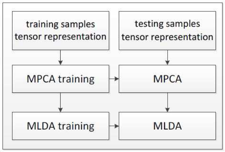
The specific algorithm flow chart is shown in Figure 1. First, each cell of all of the multi-band data is represented by a third-order tensor $R^{9\times M\times N^2}$; then, the training samples are processed with the MPCA algorithm, and the projection matrices and the projected tensors of training samples are outputted. After the subtensors are trained with the MLDA algorithm, we can get the final projection matrices and the final projected tensors of training samples. Finally, the principal components of the testing data are extracted with the projection matrices that have been trained.

Let ${{\mathbf{U}}^{(l)}|}_{l=1}^N$ be the output projection matrices with the MPCA training algorithm, ${{\mathbf{V}}^{(l)}|}_{l=1}^N$ be output projection matrices with the MLDA training algorithm and the testing tensors be X_i, (i = 1, …, M), and then, the extracting subtensors are Z_i, where:

$${\mathbf{Z}}_i={\mathbf{X}}_i{\times }_1{\left({\mathbf{U}}^{(1)}{\mathbf{V}}^{(1)}\right)}^T{\times }_2{\left({\mathbf{U}}^{(2)}{\mathbf{V}}^{(2)}\right)}^T\dots {\times }_N{\left({\mathbf{U}}^{(N)}{\mathbf{V}}^{(N)}\right)}^T$$

(13)

3.3. Classification with Neural Network

After the subtensors have been extracted by the MPCA and MLDA algorithms, we can classify data using the Frobenius distance between testing subtensors and training subtensors. Since the measure of subtensors is unstable for the multiplicative speckle of the original data, the subtensor is spread out with a vector and classified with a neural network classifier.

Let the training sample be X_i, i = 1, …, M, the extracted subtensor be Z_i, the corresponding vector be z_i, the class labels be C_i, C_i ∈ {1, …, N_c}, the output of z_i traversing the NN be y_i and the corresponding desired output vectors be c_i. Then, the training model of NN is:

$$\widehat{w}=\underset{w}{\arg \min }\left({\displaystyle \sum _i{\left(y_i\left(w\right)-c_i\right)}^2}\right)$$

(14)

where e_i = y_i(w) − c_i is the error of the i-th sample and w is the weight of the neural network.

After the NN is trained and the weight of the neural network w is obtained, the output class label of the test sample X_k is:

$${\widehat{c}}_k=\underset{j}{\arg \max }\left(y_k{}_{,j}\left(w\right)\right)$$

(15)

where y_k,j(w) is the value of the output node j for test sample X_k.

4. Experimental Results and Analysis

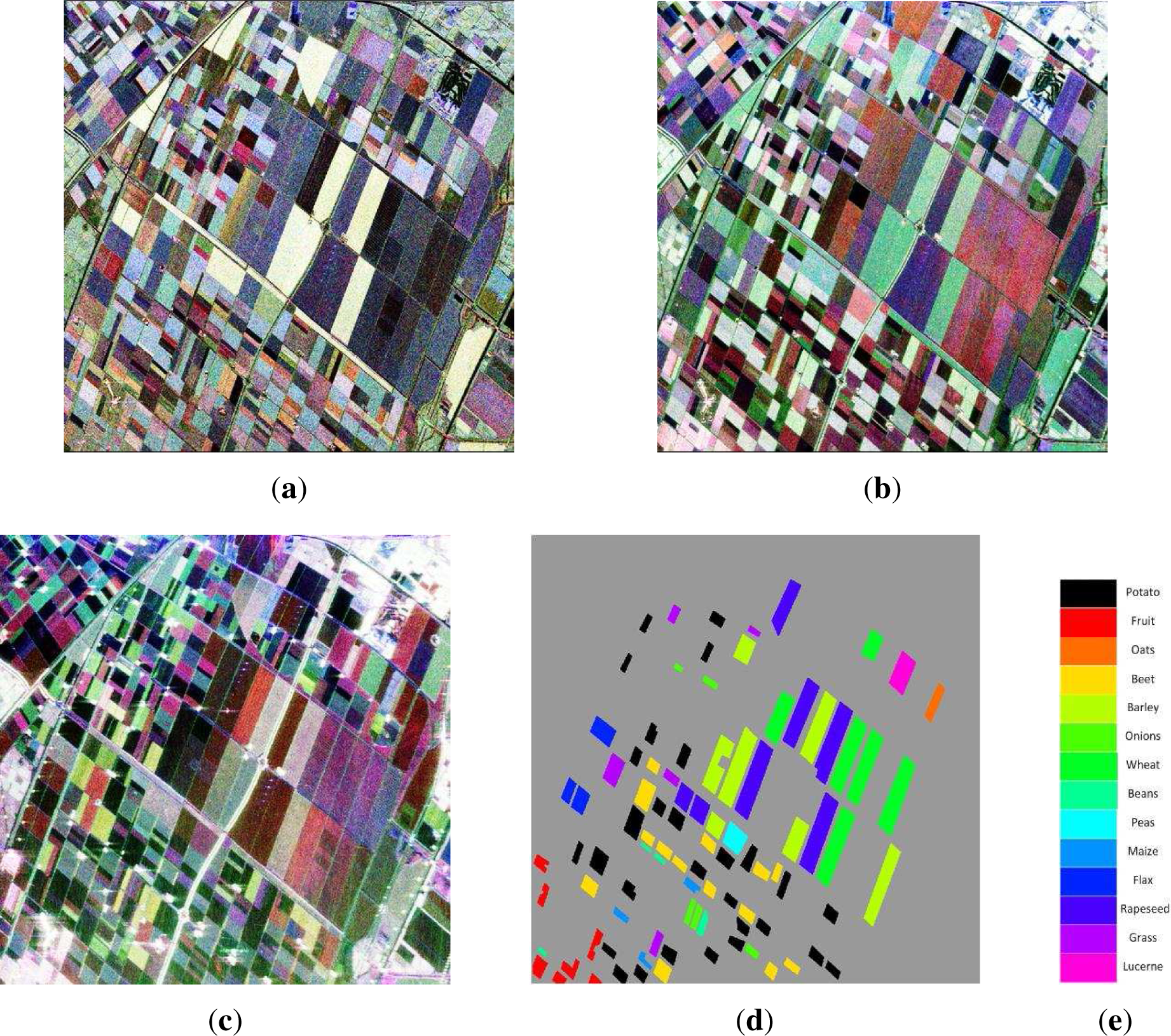
Multi-frequency polarimetric SAR images acquired by AIRSAR with the P, L and C bands, over Flevoland in the Netherlands, are used to test the performance of the proposed classification algorithm. Pauli pseudo-color images of the three bands are presented in Figure 2a–c, and the ground-truth data are shown in Figure 2d, which is drawn according to the paper of Hoekman [21]. There are 14 kinds of crops on this site, including potato, fruit, oats, and so on. Figure 2e is the types of crops and the corresponding colors in the ground-truth.

To demonstrate the effectiveness of the proposed method, three experiments are designed. In Experiment 1, we want to show the classification performance and results when the training samples are enough and the dimension of the subtensors is reasonable by setting high thresholds in both the MPCA and MLDA steps. The classification performance is compared with those of the classic Wishart classifier and the NN classifier for the tensor data, which are unfolded into a vector without dimension reducing. In Experiment 2, we want to compare the classification performance of the tensor learning method with the vector learning method, and we also want to compare the classification performances of different tensor learning methods, including the tensor learning only using MPCA and only using MLDA, as well as the proposed method. In Experiment 3, we want to show the robustness of the proposed method and the effectiveness of the extracted subtensor features, and then, the classification performance is compared when the subtensor is extracted with different thresholds in the MPCA and MLDA steps.

4.1. Experiment 1

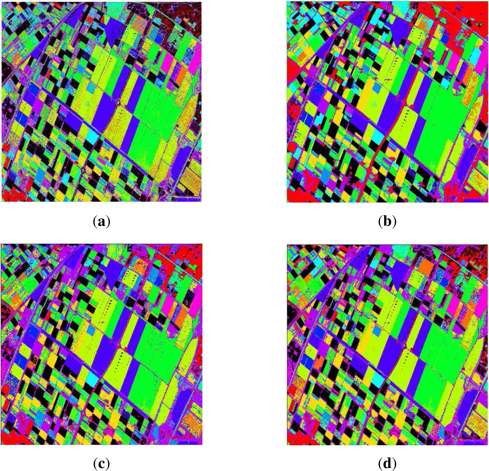
Using the same training samples, the classification performance of the proposed method is compared with the NN classification algorithm with vectors and the Wishart algorithm proposed by Lee [1], in which three bands’ data are assumed to be statistically independent. The training samples are selected randomly from the ground-truth, and 500 samples are selected for each class. The testing samples are all pixels in the ground-truth. The spatial window size is 3 × 3 in tensor representation. The threshold ρ is set to 0.99 in MPCA, and the threshold is set to 0.995 in MLDA for the proposed algorithm. The classification results are shown in Figure 3. Figure 3a is the classification result of the Wishart algorithm; Figure 3b is the classification result of the Wishart algorithm after the data have been filtered with a 3×3 window; Figure 3c is the result of the NN classifier in which the tensor data are unfolded into a vector without dimension reducing; and Figure 3d is the result of the proposed algorithm. The dimension of the original tensor is 9 × 3 × 9. After being processed with MPCA and MLDA, the dimension of the subtensor is 8×3×2.

Table 1. The classification results of the Wishart algorithm, the NN classifier with original data and the proposed algorithm (OA is the overall accuracy) (1–14 are the orders corresponding to the crop types shown in Figure 2(e): 1, potato; 2, fruit; 3, oats; 4, beet; 5, barley; 6, onions; 7, wheat; 8, beans; 9, peas; 10, maize; 11, flax; 12, rapeseed; 13, grass; 14, lucerne).

1 Trial(%)	Accuracy														OA	Kappa
	1	2	3	4	5	6	7	8	9	10	11	12	13	14
Wishart	95.6	92.7	97.3	73.8	87.4	78.1	97.1	96.8	98.2	85.4	96.5	97.7	91.4	98.2	93.1	93.7
Wishart With filtered data	99.9	99.9	99.8	93.9	99.4	72.1	99.9	98.5	100	92.3	97.0	100	82.1	99.9	98	95.8
NN classifier With original data	98.9	100	94.8	77.6	95.4	95	98	99.9	98.7	90.3	97.1	99.9	97	99.6	96.3	96.2
Proposed method	99.6	99.7	99.7	95.9	99.4	93.4	99.5	99.7	100	89	97.3	99.6	98.2	99.9	98.9	97.9

lists the classification result, including the correct rates, the total accuracies and the kappa coefficients of the confusion matrices.

From Table 1, it can be observed that the classification performance of the proposed algorithm is good. The correct rates of different crops are all higher than 95%, except corn; the overall accuracy is as high as 98.9%; and the kappa coefficient measuring the overall classification effect of the proposed algorithm is 97.9%. The performance of the proposed method is improved for all crops compared with the Wishart classifier and the NN classifier with the original data without dimension reducing, and the accuracies of some crops are improved obviously, such as beet, barley and onions. Although the overall accuracies of the proposed method and that of the Wishart classifier with the filtered data are almost equal, the accuracy rates of the classes of onion and grass are far better than those of the Wishart classifier. It can also be observed that the classification result is better than other algorithms from Figure 3. The burr of the proposed method in homogeneous areas is less than that of the Wishart algorithm. Although the classification accuracies are nearly equal, the classification accuracies are better than the NN classifier without dimension reducing and the Wishart classifier with the filtered data in the areas that are not marked in the ground-truth, especially in the grass area from Figure 3.

4.2. Experiment 2

Classification performances of the NN classifier with the two vector learning methods and three tensor learning methods are compared. The two vector learning methods are the PCA and PCA + LDA algorithms; the three tensor learning methods are the MPCA, MLDA and the proposed MPCA + MLDA algorithms. The window size is the same as that used in Experiment 1. To keep the classification performance relatively good, the average dimensions of subtensors of those five algorithms about the same and the values relatively low, the threshold of the PCA step is set to 0.9 in the PCA method, to 0.95 in the PCA+LDA method, the threshold of MPCA only to 0.9, the threshold of MLDA only to 0.99, to 0.97 in the MPCA step and to 0.99 in the MLDA step for the proposed method. The experiment is repeated 100 times. In each trial, the training samples are selected randomly, and the sample number for each crop is 300; the testing samples are all pixels in ground-truth. The average dimensions of the subvectors and subtensors of those algorithms are about the same after being processed, which is 23 for PCA, 32 for MPCA, 21 for MLDA and 21 for the proposed method. The dimension of the PCA + LDA method is determined by the number of classes.

Table 2. The classification performance of the PCA only, LDA only, multi-linear principal component analysis (MPCA) only, multi-linear extension of linear discriminant analysis (MLDA) only, the proposed method and Wishart algorithm.

100 Trials(%)	Accuracy														OA	Kappa
	1	2	3	4	5	6	7	8	9	10	11	12	13	14
PCA	95.6	99.8	96.1	82.4	89.8	94.2	96.6	99.9	94.5	86.7	92.7	99.9	94.1	97.8	94.5	94.1
PCA+LDA	96.9	99.5	91.8	80.3	89.6	95.2	94.1	99.9	96.2	82.4	95.3	99.2	73.6	92.6	93.1	90
MPCA	96.9	99.9	94.6	69.7	90.8	94.9	97.9	99.2	88	70.7	78.9	99.7	89.5	88.6	92.9	91.6
MLDA	99.3	99	99.3	88.1	97.4	88.8	98.2	99.8	99.5	78	92.6	99.7	95.5	99.2	97.1	96.1
Wishart	99	99.7	98.7	87.3	94	68.1	99.6	97	99.8	87.2	94.4	99.8	78.5	99.9	95.9	94
Proposed method	99.4	99.2	99.3	89.7	98.8	90.9	98.5	99.8	99.2	79.2	95	99.8	96.9	99.5	97.8	96.5

lists the average classification result of the different algorithms.

According to the results shown in Table 2, firstly, we can observe that the classification performances of the tensor-based learning methods are better than those of the vector-based learning methods. Secondly, for the three tensor-based learning methods, MPCA performs worse than the MLDA and the proposed method when the dimensions of the subtensors are about the same, especially in Types 4 and 11. The performance of the proposed method is slightly better than the MLDA algorithm. Thirdly, the accuracies of the proposed method are improved compared with the Wishart classifier with the filtered data for all crops, except Type 10.

4.3. Experiment 3

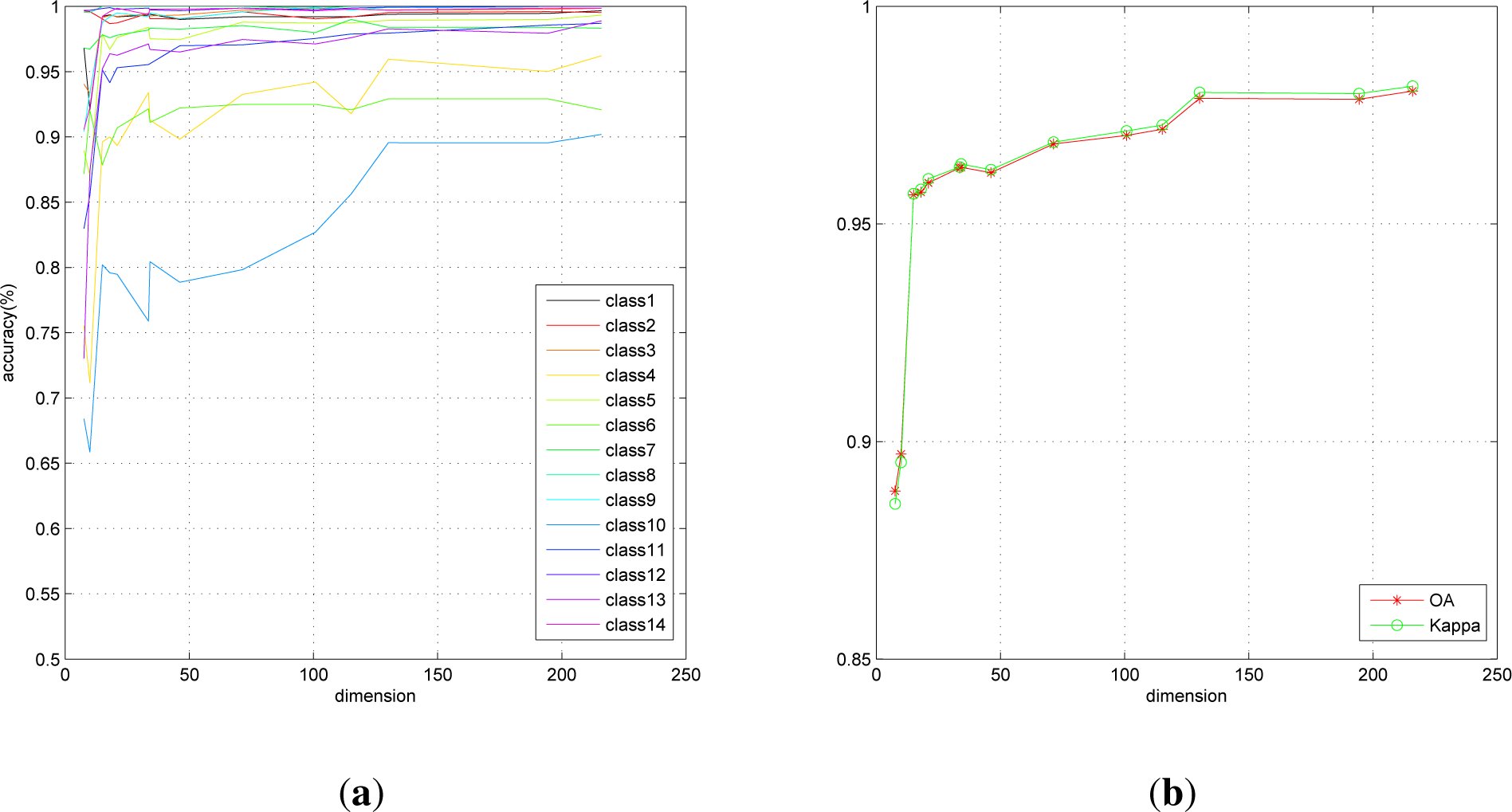
In the third experiment, the classification performance is compared when the subtensor is extracted with different thresholds in the MPCA and MLDA steps. The threshold is varying from 0.9 to 0.99 for MPCA and varying from 0.92 to 0.999 for MLDA. The training and testing samples are selected the same as in Experiment 2, i.e., 100 trials are carried out for each threshold. The variation of classification accuracies of all 14 crops along with the dimensional change of the subtensors are shown in Figure 4.

With the increase of the dimension of subtensors, the accuracies of all crops are improved gradually. The ascent rates are fast when the dimension is less than 20 and tend to be saturated after the dimension exceeds 20, except Crop 10. The variation tendency of the overall accuracy and the kappa coefficient are the same, also increasing rapidly firstly and then growing slowly. It can be observed that the classification accuracy for each crop and the overall accuracy will exceed 90% after the dimension of subtensors is higher than 20, which shows the robustness of the proposed algorithm and the efficiency of the extracted subtensor features.

5. Conclusions

Taking into consideration the characteristics of frequency, polarization and spatial domain simultaneously for the multi-frequency polarimetric synthetic aperture radar (SAR) data, we have presented a multi-frequency polarimetric SAR classification scheme based on tensor representation and multilinear subspace learning (MSL). Compared with the classic method in which the data or features are represented and learned by vector, the proposed method represents the cell of multi-band data with a third-order tensor in the directions of spatial, frequency and polarization. The principle features are extracted more precisely, and the discrimination ability of the features between classes is improved when using the multi-linear principal component analysis (MPCA) method and the multi-linear extension of linear discriminant analysis (MLDA) method. The proposed algorithm was evaluated with multi-frequency polarimetric SAR data of Airborne Synthetic Aperture Radar (AIRSAR). The classification performances of the three tensor learning algorithms, two vector learning algorithms and the classic Wishart classifier were compared. The accuracies of the proposed algorithm with the dimensional change of subtensors were also tested. Experimental results have demonstrated that the classification accuracy of the proposed algorithm is better than other algorithms; the performance is promising, even when the dimension of the extracted subtensors is low. In addition, the extracted subtensors are three-dimensional, and the overall structure of the original data in the directions of spatial, frequency and polarization is well kept.

References

- Lee, J.S.; Grunes, M.R.; Kwok, R. Classification of multi-look polarimetric SAR imagery based on complex Wishart distribution. Int. J. Remote Sens. 1994, 15, 2299–2311. [Google Scholar]
- Famil, L.F.; Pottier, E.; Lee, J.S. Unsupervised classification of multifrequency and fully polarimetric SAR images based on the H/A/Alpha-Wishart classifier. IEEE Trans. Geosci. Remote Sens. 2001, 39, 2332–2342. [Google Scholar]
- Frery, A.C.; Correia, A.H.; Da Freitas, C. Classifying multi-frequency fully polarimetric imagery with multiple sources of statistical evidence and contextual information. IEEE Trans. Geosci. Remote Sens. 2007, 45, 3098–3109. [Google Scholar]
- Gao, W.; Yang, J.; Ma, W. Land cover classification for polarimetric SAR images based on mixture models. Remote Sens. 2014, 6, 3770–3790. [Google Scholar]
- Freeman, A.; Willasenor, J.; Klein, J.D. On the use of multi-frequency and polarimetric radar backscatter features for classification of agricultural crops. Int. J. Remote Sens. 1994, 15, 1799–1812. [Google Scholar]
- Kouskoulas, Y.; Ulaby, F.T.; Pierce, L.E. The Bayesian hierarchical classifier (BHC) and its application to short vegetation using multi-frequency polarimetric SAR. IEEE Trans. Geosci. Remote Sens. 2004, 42, 469–477. [Google Scholar]
- Chen, K.S.; Huang, W.P. Classification of multifrequency polarimtric SAR imagery using a dynamic learning neural network. IEEE Trans. Geosci. Remote Sens. 1996, 34, 814–820. [Google Scholar]
- Lardeux, C.; Frison, P.L.; Tison, C.; Souyris, J.C.; Stoll, B.; Fruneau, B.; Rudant, J.P. Support vector machine for multi-frequency SAR polarimetric data classification. IEEE Trans. Geosci. Remote Sens. 2009, 47, 4143–4152. [Google Scholar]
- Lee, J.S.; Grunes, M.R.; Mango, S.A. Speckle reduction in multipolarization, multi-frequency SAR imagery. IEEE Trans. Geosci. Remote Sens. 1991, 29, 535–544. [Google Scholar]
- Lee, J.S.; Hoppel, K. Principal components transformation of multi-frequency polarimetric SAR imagery. IEEE Trans. Geosci. Remote Sens. 1992, 30, 686–696. [Google Scholar]
- Trizna, D.B.; Bachmann, C.; Sletten, M.; Allan, N.; Toporkov, J.; Harris, R. Projection pursuit classification of multiband polarimetric SAR land images. IEEE Trans. Geosci. Remote Sens. 2001, 39, 2380–2386. [Google Scholar]
- Azimi-Sadjadi, M.R.; Ghaloum, S.; Zoughi, R. Terrain classification in SAR images using principal components analysis and neural networks. IEEE Trans. Geosci. Remote Sens. 1993, 31, 511–515. [Google Scholar]
- Chamundeeswari, V.V.; Singh, D.; Singh, K. An analysis of texture measures in PCA-based unsupervised classification of SAR images. IEEE Trans. Geosci. Remote Sens. 2009, 6, 214–218. [Google Scholar]
- Ainsworth, T.L.; Lee, J.S. Optimal polarimetric decomposition variables-non-linear dimensionality reduction. IEEE Inter. Geosci. Remote Sens. 2001, 2, 928–930. [Google Scholar]
- Ainsworth, T.L.; Lee, J.S. Polarimetric SAR image classification-exploiting optimal variables derived from multiple-image datasets, Proceedings of the IEEE International Geoscience and Remote Sensing Symposium, Anchorage, AK, USA, 20–24 September 2004; 1.
- Kolda, T.G.; Bader, B.W. Tensor decompositions and applications. SIAM Rev. 2009, 51, 455–500. [Google Scholar]
- De Lathauwer, L.; de Moor, B.; Vandewalle, J. On the best rank-1 and rank-(r 1, r 2,…, rn) approximation of higher-order tensors. SIAM J. Matrix Anal. Appl. 2000, 21, 1324–1342. [Google Scholar]
- Lu, H.; Plataniotis, K.N.; Venetsanopoulos, A.N. MPCA: Multilinear principal component analysis of tensor objects. IEEE Trans. Neural Netw. 2008, 19, 18–39. [Google Scholar]
- Yan, S.; Xu, D.; Yang, Q.; Zhang, L.; Tang, X.; Zhang, H.J. Discriminant analysis with tensor representation, Proceedings of the IEEE Computer Society Conference on Computer Vision and Pattern Recognition, San Diego, CA, USA, 20–26 June 2005; 1, pp. 526–532.
- Tao, D.; Li, X.; Wu, X.; Maybank, S.J. General tensor discriminant analysis and gabor features for gait recognition. IEEE Trans. PAMI 2007, 29, 1700–1715. [Google Scholar]
- Hoekman, D.H.; Vissers, M.A. A new polarimetric classification approach evaluated for agricultural crops. IEEE Trans. Geosci. Remote Sens. 2003, 41, 2881–2889. [Google Scholar]