Reliable Crop Identification with Satellite Imagery in the Context of Common Agriculture Policy Subsidy Control

Abstract

Agricultural subsidies in the context of the Common Agricultural Policy (CAP) represent over 40% of the EU’s yearly budget. To ensure that funds are properly spent, farmers are controlled by National Control and Paying Agencies (NCPA) using tools, such as computer-assisted photo interpretation (CAPI), which aims at identifying crops via remotely-sensed imagery. CAPI is time consuming and requires a large team of skilled photo interpreters. The objective of this study was to develop a reliable control system to partially replace CAPI for crop identification, with the overreaching goal of reducing control costs and completion time. Validated control data provided by the Portuguese Control and Paying Agency and an atmospherically-corrected Landsat ETM+ time series were used to perform parcel-based crop classification, leading to an accuracy of only 68% due to high similarity between crops’ spectral signatures. To address this problem, we propose an automatic control system (ACS) that couples crop classification to a reliability requirement. This allows the decision-maker to set a reliability level, which restricts automatic crop identification to parcels that are classified with high certainty. While higher reliability levels reduce the risk of misclassifications, lower levels increase the proportion of automatic control decisions (ACP). With a reliability level of 80%, more than half of the parcels in our study area are automatically identified with an overall accuracy of 84%. In particular, this allows automatically controlling over 85% of all parcels classified as maize, rice, wheat or vineyard.

1. Introduction

In this section, the problem we address is described, and the main motivations and goals of this research are discussed. The reader can find a list of the most important acronyms at the end of the paper.

1.1. Use of Remote Sensing for CAP Subsidy Control

The Common Agricultural Policy (CAP) is a system of European Union (EU) agricultural subsidies and programs that is very significant in financial terms, representing over 40% of the EU’s budget, equivalent to €58 billion in 2011 [1]. To ensure that CAP funds are spent appropriately, Member State Authorities have to comply with legal management and control mechanisms [2]. Toward that end, European Commission (EC)’s Joint Research Centre (JRC) provides technical support to Member States. To date, Control with Remote Sensing (CwRS), Digital Land Parcel Identification System (LPIS) and parcel area measurement using Global Navigation Satellite Systems (GNSS) devices have become the keystones of the efficient administration and control of CAP subsidies [3]. Each Member State is responsible for subsidy administration and control, which are carried out by a National Control and Paying Agency (NCPA).

In order to obtain area-based financial support, farmers are required to submit an application to their NCPA early in the year, where they declare the precise location of all of their agricultural parcels, as well as the crop type. The National Agency is responsible for controlling at least 5% of those declarations and penalizing farmers who submit incorrect information by performing so-called On-The-Spot (OTS) checks. For area-based subsidies, an agricultural parcel must be controlled at two different levels: both the declared crop and area must be correct [4]. The EC in turn controls the NCPAs. When discrepancies between the control result and the reality are found, a Member State is penalized and has to return to the EU part of the subsidies that were distributed to farmers.

The complex process of subsidy control requires computational tools: NCPAs rely on Integrated Administration and Control System (IACS)s, which includes a LPIS. The main functions of those spatial databases are localization, identification and quantification of agricultural land via detailed geospatial data, in order to facilitate the distribution of CAP subsidies [5].

CwRS, the goal of which is to perform OTS checks “in the office” as much as possible, has become an official method for NCPAs to carry out part or all of their OTS checks of EU farms [2]. It uses remotely sensed data, which are acquired by the EU and distributed to the NCPAs by JRC. The CwRS program enabled in 2013 the control of over 400,000 farmers’ area-based subsidy applications and represented 70% of the EU OTS checks [3]. NCPAs have been relying on Computer Assisted Photo-Interpretation (CAPI) of High Resolution (HR) and Very High Resolution (VHR) imagery time series to perform CwRS. However, CAPI is time consuming; it depends on the skills of the photo interpreters and requires a large team. Therefore, there is an obvious need for the development of cost-effective methods to automatize crop identification, which are essential for control in the context of area-based agricultural subsidies, in order to lower costs, speed up work and improve reliability compared to CAPI [4,6]. However, the accuracy of automatic classification in an operational context is critical and must be taken into account during the development of such automatic identification methodologies.

1.2. Parcel-Based Crop Identification

Multitemporal and multispectral remote sensing imagery has been widely used for crop identification in past years [7,8] since time series of satellite images are believed to be a cost-effective data source to assess land cover, such as agricultural crops over large areas [9]. The basis for separating one crop from another is the supposition that each crop species has a specific spectral signature in a time series of multispectral images. However, major limitations on crop identification with satellite imagery, like the similarity of the plant reflectance of different crops, parcel-to-parcel variability of the plant reflectance of the same crops and changes in the pattern of individual crop phenology, may occur [8].

Pixel-based classification approaches, where pixels are classified individually regardless of their spatial aggregation, generally lead to poor results [8,10]. To overcome this problem, object-based techniques have been increasingly used in remotely-sensed image analysis. Object-Based Image Analysis (OBIA) typically relies on segmentation algorithms to define geographical objects that can be classified; this is known as “object-based classification” [10,11]. However, when a spatial database, such as the LPIS, is available, segmentation algorithms might not be necessary, since agricultural parcels extracted from LPIS can in principle be used instead of objects resulting from image segmentation; this is what we call “parcel-based classification”. The operational applicability of parcel-based approaches is conditioned by the geographic information available in the national LPIS. As described in [5], the LPIS Conceptual Model (LCM) requires the geometry of the reference parcel to be stored. However, and depending on the type of reference parcel used by each Member State, it might not represent a single crop. As discussed in [5], the LCM class Reference Parcel is associated with a land cover type, which includes, among others, arable land, irrigated rice or grassland, but information about specific crops, like wheat or barley, are stored in a separate class (Agricultural Parcel) with no geometry. To complicate matters, the reference parcel might include very small non-eligible features. Nonetheless, the location of individual agriculture parcels is included in LPIS, in the form of the farmer’s sketch, as required by EU regulation [12]. When this information is available in digital format, it can be used for parcel-based crop identification. Moreover, some classes of interest for aid application correspond to land cover types (e.g., vineyard) and are therefore represented geometrically in LPIS.

Several studies have been conducted on automatic crop identification in the context of CAP subsidies using object and parcel-based image classification. Matikainen et al. [13] developed a method for automatic change detection in the Finnish LPIS. They used segmentation of aerial orthoimagery inside of each of the LPIS parcels. Each of the resulting objects were classified with a decision tree and then compared to detect changes. Their results suggest that real changes in LPIS can be detected relatively well, but a large number of false detections occur. Blaes et al. [4] developed a parcel-based strategy for crop identification in the operational context of subsidy controls. Those authors used farm plot outlines digitized from farmers’ declarations and determined the best combination of acquisition dates and image sensors, including radar sensors, that maximize the detection of incorrect farmer’s declarations. Oesterle and Hahn [14] also used segmentation of VHR aerial orthoimagery to investigate the automatic update of the German LPIS.

1.3. Reliable Crop Identification

Given the large amounts of funds involved in the CAP and the risk of penalization by the EC, it is crucial that automatic crop identification is as precise as possible in the context of operational subsidy control. We believe that the conventional “one size fits all” approach, where the crop classification is applied to all parcels, is not appropriate to develop a control system that produces reliable results. Instead, the automatic approach should be able to identify the largest possible set of agriculture parcels that can be automatically and correctly classified as determined by a reliability level set by the decision-maker. The remaining parcels, in turn, should be subjected to visual analysis in the form of CAPI or farm visits, since this is the only form to guarantee the quality of the decision process.

1.4. Objectives of the Study

The goal of this study was to develop a simple and cost-effective Automatic Control System (ACS) to automatize the control process and reduce OTS check costs and completion time. The proposed solution consists of the automatic classification of as many agricultural parcels as possible, eliminating the need of CAPI for controlling those parcels. Our ACS comprises a reliability level, chosen by the decision-maker, which allows our approach to focus on parcels that can be classified automatically with high certainty. For those parcels, we performed a parcel-based classification of multispectral and multitemporal land cover signatures retrieved from remotely-sensed imagery, taking advantage of the object-based nature of agricultural parcels. We used field-validated OTS check data from the Portuguese NCPA (Instituto de Financiamento da Agricultura e Pescas (IFAP)) and an atmospherically-corrected multispectral Landsat 7 Enhanced Thematic Mapper (ETM+) time series to develop and train our methodology for twelve major land cover classes in the Portuguese Ribatejo agricultural landscape.

Although this study responds to a practical problem raised by the Portuguese NCPA, our approach is conceptual and could be in principle applied to different areas, crops and remote sensing imagery. Our case study happens to be situated in an area with a Mediterranean climate, where cloud-free images are typically available with high temporal resolution during a large part of crops’ development cycles (spring and summer). However, our ACS could be used as long as a dense time series of images is available for the area of interest. In particular, SAR data could be combined with optical imagery for cloud-persistent regions, as in [4].

2. Study Area and Datasets

2.1. Study Area Description

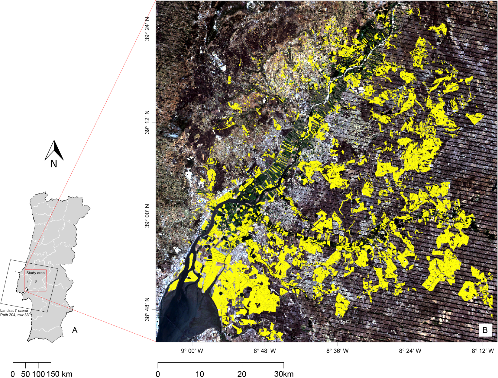
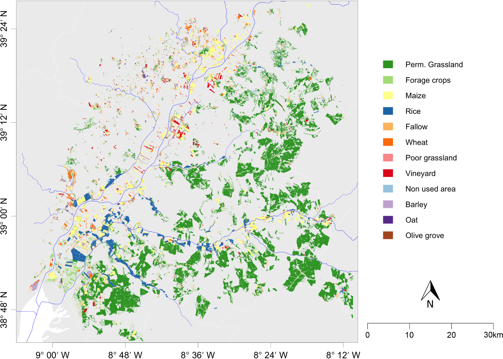
The study area is located within the Portuguese province Ribatejo, northeast of Lisbon, including mainly parts of the Lisbon and the Santarém districts (Figure 1). It extends over an area of about 6390 km² and is situated between longitudes 9°6′0″W and 8°9′36″W and latitudes 38°43′47″N and 39°27′36″N (Datum WGS84). Agriculture is the main activity in Ribatejo with a wide range of different commodities, containing some of Portugal’s richest agricultural land. This agricultural area is situated within the Tagus River basin, which plays an important role for both the agricultural activity and climate of the region. The Tagus River is also responsible for the relatively flat relief of the whole study area, with a height ranging between zero and 200 m above sea level. The study area is characterized by a Mediterranean climate with long hot and dry summers and moderate, rainy winters. On average, annual mean temperature is between 15 °C and 16 °C and rainfall ranges from 600 to 800 mm/year, with many crops being irrigated during the dry summer growing season. The very diverse cropping pattern found in the Ribatejo province was the main reason that this area was selected for our study, along with the good availability of field-validated OTS control data from IFAP.

2.2. Remote Sensing Data

Table 1. Optimal periods for image acquisition according to Carmona [15] used by IFAP and acquisition dates of Landsat ETM+ images selected for this study (date formats: dd/mm and dd/mm/yyyy).

N	Optimal Period	Acquisition Date
Period 1	15/10 to 15/11	10/11/2004
Period 2	15/02 to 03/15	14/02/2005
Period 3	15/04 to 15/06	05/05/2005 06/06/2005
Period 4	01/07 to 15/07	08/07/2005
Period 5	01/08 to 08/07	28/08/2005

shows the five optimal periods used for multitemporal image acquisition by IFAP to perform CAPI [15]. IFAP usually requests one HR image per period to JRC. These periods were chosen in order to optimally follow the annual agricultural cycle of both winter and summer crops cultivated in Portugal. Images for this study were also screened for atmospheric effects and clouds.

Based on these criteria, six Landsat-7 ETM+ multispectral images over the study area (WRS-2 Path 204, Row 33) from a period between November 2004 and August 2005 were acquired through USGS EarthExplorer (Table 1). The imagery consisted of atmospherically-corrected surface reflectance data (climate data records), generated from the LEDAPS tool. LEDAPS uses MODIS atmospheric correction routines and complex 6S radiative transfer models in order to generate surface reflectance [16]. The six visible and short-wave infrared bands (Bands 1 to 5 and 7) with a spatial resolution of 30 m were used. The bands from all multispectral images in the temporal sequence (six bands for each image) were stacked, forming a single multi-date image with 36 bands. Landsat data was primarily chosen due to its cost-effectiveness and good temporal coverage. In addition, Landsat ETM+ imagery is known to be appropriate for detailed large-area crop mapping [17]. We were limited to Landsat 7 ETM+ imagery for this study, since no other Landsat images were available at EarthExplorer for the study area and period.

All acquired images were affected by the Scan Line Corrector (SLC)-off issue, which results in the loss of approximately 22% of the normal scene area for Landsat ETM+ acquisitions after 31 May 2003. However, the SLC-off issue has no impact on the quality of the remaining valid pixels [18]. The study area covered only a relatively small portion of the scenes, including their central part, and was therefore not highly affected. More precisely, only 12.6% of the pixels within the analyzed crop parcels had “fill-values” in the images provided by USGS. Those pixels were ignored in further processing steps.

2.3. Agricultural Parcels and Crop Classes

Field validated data from agricultural parcels controlled in 2005 in the context of CAP were used in this study to develop and train our ACS. IFAP produced this data by OTS checks through CAPI, followed by farm visits when necessary. Since the Portuguese LPIS in 2005 represented single crop parcels (Figure 7 in [12]), which were refined through field validation, boundaries of single crops were available for this study. The year 2005 was chosen due to the relatively high control rate in Ribatejo in that year, allowing us to analyze a broad range of different crops, as mentioned before. After 2005, CAP’s Single Payment Scheme, which decoupled subsidies from the production of specific crops, was progressively adopted by Portuguese farmers, with the consequence of reducing the diversity of declared crops.

A total of 32,062 agricultural parcels lying within the study area were initially provided by IFAP. Only pixels lying entirely within a parcel were considered in order to avoid mixed pixels at the boundary. A subset of the initial parcels was then selected for further analysis based on two criteria. Firstly, all parcels had to contain at least one entire pixel. Secondly, only parcels containing crop classes accounting for approximately 95% of the total parcel area were included in the subset. In detail, 12 classes (

Table 2. Summary of the used crop classes. More than half of the area is covered by permanent grassland. Note the great variability in parcel size found in the data (measured as the standard deviation of the parcel area).

Land Cover Class	Class Label	Number of Parcels	Total Area (ha)	Average Area (ha)
Permanent grassland	PGL	4051	59,243	14.6 ± 13.9
Forage crops	FOR	1708	12,183	7.1 ± 8.2
Maize	MAI	1190	8916	7.5 ± 6.5
Rice	RIC	799	6501	8.1 ± 6.9
Fallow	FAL	1473	5944	4 ± 5.1
Wheat	WHE	578	2710	4.7 ± 4.8
Poor grassland	POG	330	2707	8.2 ± 10.4
Vineyard	VYA	578	2197	3.8 ± 3.6
Non used area	NUA	329	1727	5.2 ± 9.8
Barley	BAR	275	1645	6 ± 6.4
Oat	OAT	282	1189	4.2 ± 5.4
Olive grove	OLI	259	741	2.9 ± 3

) covered 94.4% of the total parcel area of 111,963 ha, with the remaining 5.6% being covered by 48 classes. This resulted in a total of 11,852 parcels used for this work, representing 105,702 ha of the study area. Of those parcels, 68.5% were not at all affected by the SLC-off problem of Landsat ETM+. Note that, strictly speaking, our 11,852 parcels do not reflect with certainty the most cultivated crops in the region, but the most controlled crops in 2005 in the study area.

3. Methods

In simple terms, the proposed ACS is a classifier coupled with a reliability requirement. In Section 3.1, we describe the techniques used for variable selection. The ACS itself is divided into three steps: classification, which is done by an SVM classifier using 10-fold cross-validation (Section 3.2); calibration, which is at the core of our approach and is described in Section 3.3; and application in an operational context (Section 3.4). Finally, in Section 3.5, we explain how we assess the proposed ACS. Figure 2 shows the three processing steps, as well as their data inputs and outputs. All data processing steps were performed using the freely-available software environment R, Version 3.0.2 [19].

3.1. Variable Selection

Each single parcel is described by the set of pixel reflectances in its interior, and each pixel is observed in several spectral bands and dates. Therefore, the dimensionality is very high, which means that feature selection is required. This is done at two levels. Firstly, we discuss how the set of pixel measurements within the parcel can be reduced. Then, we discuss how to select the best set of combinations of spectral bands and acquisition dates from the 36 possible combinations (6 bands and 6 dates). Dimensionality reduction is a common preprocessing step in supervised classification, since it prevents possible redundancy in the datasets and overfitting [20]. Moreover, dimensionality reduction may permit reducing the amount of data (fewer acquisition dates) and computational effort.

To address the first issue of within-parcel measurements, we compared the variability between parcels with the variability within parcels for each combination of band and date. Our goal was to investigate if the variability between parcels was much higher than within parcels, which is expected for parcel-based classification where parcels are homogeneous. Since our population includes several crops, we decomposed the total variability, for all pixels within the 11,852 parcels, as in a two-way nested ANOVA, where crops are the main factor and parcels are the nested factor. This allows us to isolate the crop effect and to compute the quotient:

$$F_{\text{Parcels}}=\frac{\text{between-parcel mean square}}{\text{within-parcel mean square}}.$$

(1)

which measures only the effect of the parcels on the overall reflectance variability. A high F-value suggests that single parcels are homogeneous and that variability among pixel reflectances is mostly due to differences between parcels. Moreover,

$$\text{RMSE}=\sqrt{\text{within-parcel mean square}}$$

(2)

measures the standard deviation within parcels. A low RMSE means that the set of all pixel reflectances within each parcel can be replaced, without much information loss, by its simple average. We stress that this analysis is simply descriptive, since parcels were not selected according to a sampling design.

To address the second level of dimensionality reduction, we performed a variable selection based on Principal Component Analysis (PCA) over the initial 36 variables (X₁). Our goal was to select the best set of original variables (the best pairs of bands and dates). However, standard PCA returns a set of orthogonal linear combinations of the variables. To obtain a set of original variables from PCA, we applied an iterative technique based on Jolliffe [21], which allows us to exclude in each step the least important variable, until linear dependencies within the dataset start to vanish. As a result, a subset X₂ of variables was generated. Since PCA only explores linear combinations of variables, it does not guarantee that a non-linear classifier will always perform better over X₂ than X₁. Therefore, we also compared the accuracy of classification over X₁ and X₂.

3.2. Classification Step

Parcel-based crop classification was carried out using the SVM classifier with X₁ and X₂ as training data. SVM have been successfully used in remote sensing applications [22,23]. This classifier is particularly attractive due to its ability to successfully handle small training datasets and for being less susceptible to problems of overfitting than other methods [24,25]. The Radial Basis Function (RBF) was used as the kernel function, because it has fewer parameter values to define and has been found at least as robust as other kernel types for remote sensing applications [24]. The SVM parameters C and ϒ were set by performing an optimum parameter search using 10-fold cross-validation.

In the classification process, a classifier assigns an object to a class based on known input variables describing the object, x. This is the classification decision. We also consider the posterior probabilities derived from SVM according to [26]. Those are the probabilities P(ω_j|x). of the true class being ω_j given x [27]. For example, P(“wheat”|x) denotes the estimated posterior probability of a parcel being a wheat crop when its signature is x. For the i-th parcel, p_i denotes the posterior probability for the most likely class. Therefore, {p₁, …, p_k} are the posterior probabilities of the k classification decisions, with k being the number of parcels in the training dataset.

An important concern in remote sensing applications is to quantify the agreement between the performed classification and ground truth data by performing accuracy assessment [6]. Accuracy assessment was undertaken using the error matrix approach [28]. Robust estimates of the error matrix, Overall Accuracy (OA), Producer’s Accuracy (PA) and User’s Accuracy (UA) for each dataset were obtained using 10-fold cross-validation. Note that PA is related to the commonly-used omission error (error of exclusion), defined as 1 – PA, while UA is related to commission error (error of inclusion), which is 1 – UA. In summary, the classification step features the following inputs and outputs:

• Input: dataset X;

• Outputs: classifier, error matrix, maximum posterior probabilities {p₁, …, p_k}.

3.3. Calibration Step

As outlined before, it is crucial to take into account the accuracy of automatic crop classification in the operational context of CAP subsidy controls, in order to build a system that produces reliable results. The rationale behind our approach is that attempting to automatically classify all parcels will inevitably lead to poor classification accuracies, at least for some classes. Our ACS allows us to control the commission errors of crop classification by using a reliability level A. The reliability level is a user-defined lower bound on user’s accuracy for all classes and can be described as an “overall UA”.

Some classification results are more reliable than others, as revealed by their respective posterior probabilities P(ω_j|x). The calibration of the control system is done by excluding parcels that were classified with low reliability, i.e., with low posterior probabilities, until the user’s accuracy in each class matches the user-defined reliability level. As a result, UA ≥ λ is guaranteed over all classes for the selected subset of parcels.

In practice, after λ is chosen, the calibration step determines a minimum posterior probability for each class, {q₁, …, q_c}, above which a classification is considered reliable (with c being the number of classes). Generally speaking, the higher the value of q_j, the more difficult it is to make a reliable decision regarding class j. In Section 4, we discuss why UA, and not PA, is the correct criterion for the calibration step. The calibration step requires and produces the following inputs and outputs:

• Inputs: reliability level λ, error matrix, maximum posterior probabilities {p₁, …, p_k};

• Output: required posterior probabilities {q₁, …, q_c}.

3.4. Application Step

The ACS is designed to be used by a control agency in an operational context in the application step once it was successfully calibrated. It is applied to each new parcel with some signature x derived from an atmospherically-corrected multispectral imagery time series and the parcel’s location.

In the application step, a given parcel is classified using the trained SVM classifier. The ACS then accepts or rejects that classification decision, with the chosen reliability level, according to the following decision rule:

$${\text{If}\omega }_j\text{is the decision, then}\{\begin{array}{c}\text{Accept decision if}P{(\omega }_j\text{|x)}\ge q_j\\ \text{Reject decision if}P{(\omega }_j\left|x\right)<q_j\end{array}$$

(3)

where P(ω_j|x) is the posterior probability and q_j is the lower bound of the posterior probability for class j defined in the calibration step. Accepting a classification decision means that the corresponding parcel can be controlled automatically by the system, while rejecting it means that the parcel does not meet the desired reliability Rejected parcels need to be subjected to CAPI. The following summarizes the application step for a given parcel:

• Inputs: classifier, required posterior probabilities {q₁, …, q_c}, signature x;

• Output: accept or reject classification decision for parcel with signature x.

3.5. Automatic Classification Proportion

For the purpose of assessing the ACS calibrated with a given reliability level, accuracy statistics OA, PA and UA were estimated only for the parcels that could be classified automatically Moreover, to measure the degree of applicability of our ACS, i.e., the proportion of parcels that can be reliably classified, we defined the Automatic Classification Proportion (ACP) for each class as follows:

$${\text{ACP}}_j=\frac{\mathrm{No}.\text{parcels classified in class}j\text{with}P{(\omega }_j|x)\ge q_j}{\mathrm{No}.\text{parcels classified in class}j}$$

(4)

the overall ACP is computed by simply dividing the total number of automatically-classified parcels by the total number of parcels.

4. Results and Discussion

4.1. Variable Selection

As described in Section 3, we performed a variance decomposition to investigate if pixel reflectances within each parcel and for each combination of ETM+ bands and acquisition dates could be replaced by the average reflectances within the parcels. Towards that end, we determined F_parcels in Equation (1) for each band and date combination. The F-values were always high (between 25.8 and 62.8) for the combinations we used for classification, as shown in

Table 3. F_parcels (left columns) and RMSE (right columns) statistics for 12 selected ETM+ band/date combinations for dimensionality reduction. F_parcels compares between-parcel with within-parcel variability after removing the crop effect, while RMSE measures the within-parcels standard deviation.

	10 November	14 February	5 May	6 June	8 July	25 August
Band 1(0.452–0.514 μm)						34.3 0.011
Band 2 (0.519–0.601μm)
Band 3 (0.631–0.692 μm)	31.2 0.016		44.7 0.018	44.7 0.018
Band 4 (0.772–0.898 μm)	45.9 0.025	63.2 0.027	62.8 0.022	51.9 0.02	49.6 0.024	45.8 0.022
Band 5 (1.547 –1.748 μm)					25.8 0.037
Band 7 (2.065–2.346 μm)		37.4 0.03

, which indicates that variability within parcels is at least 25-times lower than variability between parcels. In addition, RMSE values show that the overall standard deviation of pixel reflectance values with respect to the parcels’ average range between 0.011 and 0.037 units of reflectance, i.e., just 1.1% to 3.7%, for the combination of bands and dates we used for classification. Those results suggest that replacing the whole set of reflectance values within a parcel by the parcel’s average reflectance can be done without losing relevant information.

To select the best combinations of ETM+ bands and acquisition dates, we performed the PCA-based analysis described in Section 3. As a result, we obtained twelve combinations X₂ out of the 36 original combinations X₁. The subset X₂ is also described in Table 3. From a remote sensing perspective, the results of the selection of the best combinations of spectral bands and acquisition dates are not surprising, since the Near Infrared (NIR) spectral region (Band 4) was always selected, and the “red” band was chosen for three distinct dates.

4.2. SVM Classification

Classification was performed SVM with X₁ using C = 1.5 and γ = 0.4 and with X₂ using C = 2.5 and γ = 0.4. This indicates that with reduced dimensionality, we need to increase the penalty for misclassification errors in order to achieve good classification results. Analyzing the effect of dimensionality reduction, we found that the classifications yielded OA values of 68.4% and 68.11% for X₁ and X₂, respectively. Given these almost identical results and the aforementioned advantages of dimensionality reduction, we considered that X₂ was the best option for the next steps, in particular calibration and application.

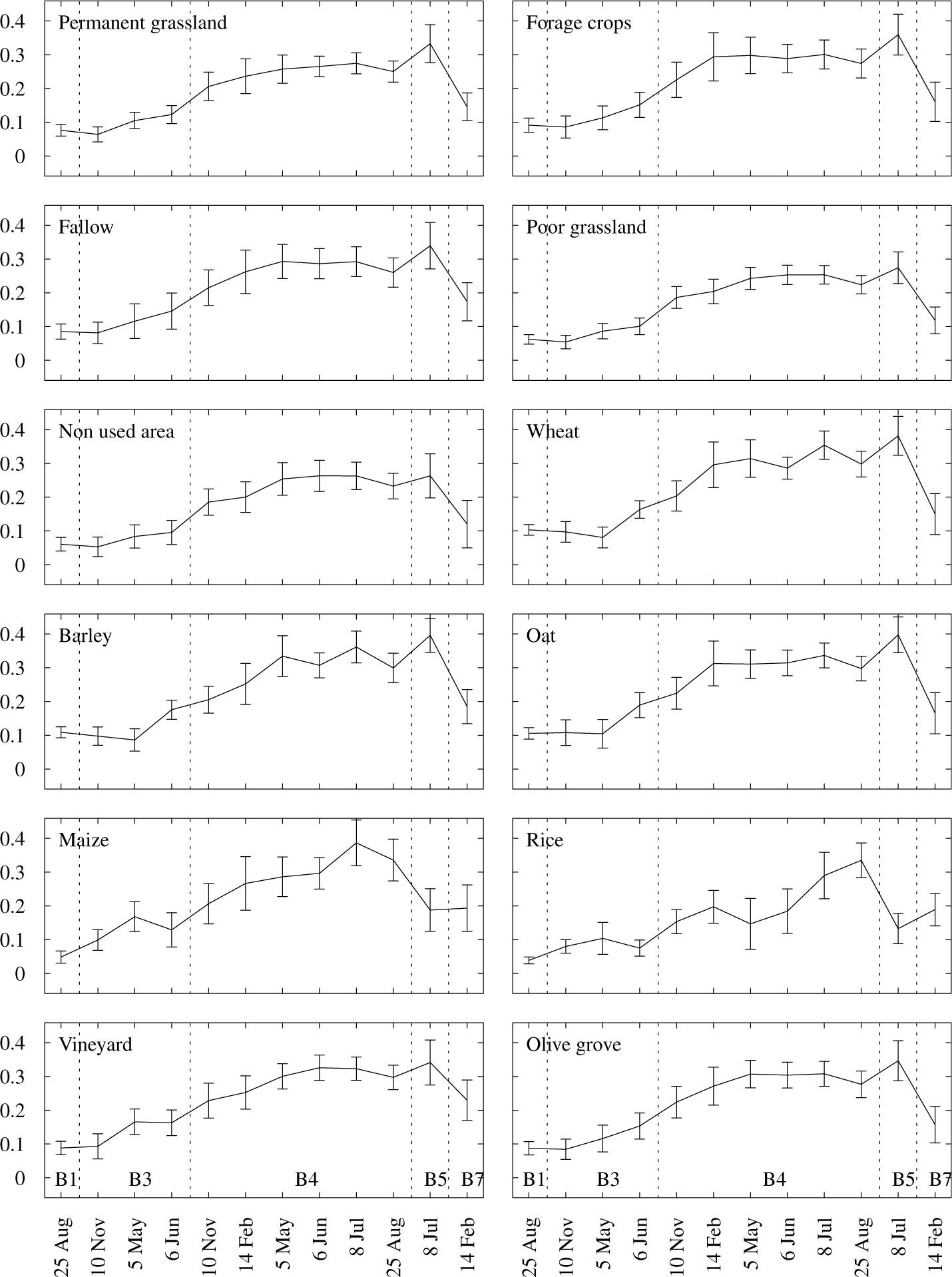
Generally speaking, OA results were rather unsatisfactory with both datasets. This confirms that attempting to classify all parcels leads to poor results. Specifically, our results show that classification OA was significantly lower than accuracies reported by other authors also performing object-based crop classification. Peña et al. [23] yielded 88% accuracy of SVM classification of nine different crops. Duro et al. [22] reported an OA of 94% with six different classes, also using the SVM classifier. Conrad et al. [7] classified six crops with an OA of 80.1%. Castillejo-González et al. [6] reported an OA of 90.7 with 10 land cover classes, mostly crops. Our classification accuracy is lower due to the fact that some of our classes are spectrally very similar, as can be seen in the spectral signatures in Figure 3. The reason for this behavior is that some classes represent very similar land cover, such as forage crops, fallow, poor grassland and non used area, and are therefore very difficult to discriminate. Cereal crops (wheat, barley and oat) also show a similar spectral pattern. However, those classes are the ones that the Portuguese NCPA currently identifies by CAPI, and therefore, the real problem at hand is intrinsically difficult. As we will see, our ACS will still lead to high accuracies.

4.3. Effect of the Reliability Level on ACP

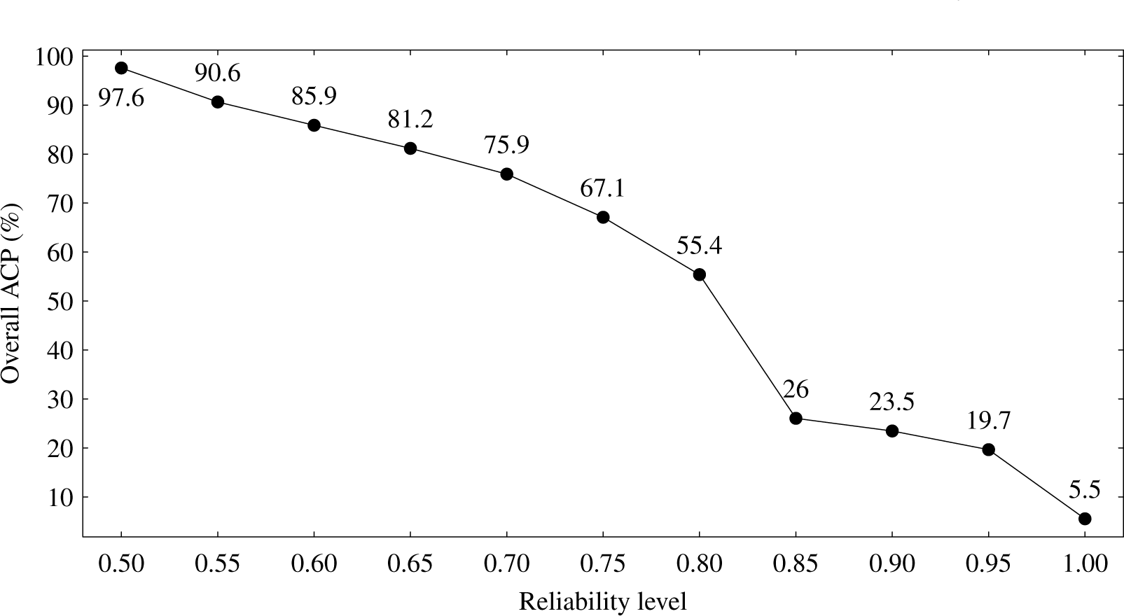
In this section, we analyze the effect of the reliability level on the proportion of agriculture parcels that can be classified automatically. This information is crucial to make a decision regarding the reliability level to adopt for automatic classification. The ACS was calibrated with λ ranging from 50% to 100%, with a 5% step, using the classification results with X₂. ACP and overall ACP were estimated for each reliability level.

The relationship between reliability level and overall ACP is shown in Figure 4. As expected, overall ACP decreases as the reliability level increases. This happens because higher reliability levels result in higher q_j values, which according to the system’s decision rule will inevitably lead to less accepted parcel classification decisions. With a low reliability level of 50%, almost all parcels can be classified automatically (97.6%). However, this is not acceptable from the perspective of subsidy control. On the other hand, if a 100% accurate classification is demanded, only 5.5% of all parcels can be classified in an automatic way. This would in fact be more accurate than CAPI, since photo interpretation is known not to be in general 100% reliable [28]. An interesting reliability level is 80%, which leads to classification errors below 20% and classifies more than 50% of all parcels in an automatic way.

The relationship between reliability level and ACP for each individual land cover class is described in Figure 5. The general trend visible in Figure 4 is obviously also present here: higher λ values lead to lower ACP values. In particular, more than 85% of maize (MAI), rice (RIC), wheat (WHE) and vineyard (VYA) parcels can be controlled using λ = 80%.

4.4. Accuracy Assessment of the ACS

For the purpose of describing and assessing ACS results for all classes, we considered a reliability level of 80%.

Table 4. Error matrices and accuracy statistics UA, PA and OA for crop classification: all parcels (top) and parcels with reliability level λ = 80% (bottom). Note that the chosen reliability level is reflected in the UA ≥ 80% yielded in each class in the second error matrix.

	Ground Truth												UA (%)
	PGL	FOR	FAL	POG	NUA	WHE	BAR	OAT	MAI	RIC	VYA	OLI
PGL	3609	633	451	258	193	4	2	29	2	1	54	66	68.1
FOR	209	700	250	3	9	56	36	98	14	1	28	59	48
FAL	147	227	626	22	38	36	9	31	17	5	60	53	49.4
POG	13	1	2	14	13								30.1
NUA	21	3	7	31	59					3		6	44.9
WHE	4	30	15		2	429	49	34	2			1	76.1
BAR	2	14	5			32	169	11				1	72.2
OAT	2	25	8		1	10	8	73	1			4	52.7
MAI	13	32	42		5	9	2	5	1141	16	4		90
RIC	1		1		4				7	772			98.4
VYA	23	35	54		5	1			6	1	428	17	75.2
OLI	7	8	12	2		1		1			4	52	59.5
PA (%)	89.1	41	42.5	4.2	17.9	74.2	61.4	25.9	95.9	96.6	74	20.1	OA = 68.1
													ACP = 100
PGL	2563	264	138	129	77			9			8	15	80
FOR	7	73	5			2	1	3					80.2
FAL													n.d.
POG				1									100
NUA					2								100
WHE	2	19	12		2	402	35	27	2			1	80.1
BAR		6	1			20	132	6					80
OAT		4	1					20					80
MAI	13	32	42		5	9	2	5	1141	16	4		89.9
RIC	1		1		4				7	772			98.3
VYA	15	22	41		2	1			4	1	394	12	80.1
OLI	2	1	3									24	80
PA (%)	98.5	17.3	0	0.8	2.2	92.6	77.6	28.6	98.9	97.8	97	46.2	OA = 84.1
													ACP = 55.4

compares error matrices and accuracy statistics for crop classification of all parcels and classification of parcels with λ = 80%. The transition from the first to the second error matrix provides a good idea of how the calibration step works. The parcels that were removed from the first error matrix are parcels with posterior probability below the required q_j determined by the calibration step. A summary of q_j and ACP values for λ = 80% is provided in

Table 5. Estimates of q_j and ACP, both with a reliability level λ = 80%.

Class	PGL	FOR	FAL	POG	NUA	WHE	BAR	OAT	MAI	RIC	VYA	OLI
qj	0.722	0.686	n.d.	0.636	0.733	0.407	0.487	0.683	0.239	0.257	0.426	0.492
ACP (%)	60.4	6.2	0	2.3	1.5	88.7	70.5	18.9	100	100	86.3	34.5

.

The ACS allowed improving the classification OA from 68.1% to 84.1%. However, this improvement comes with the cost of reducing the proportion of parcels that can be automatically controlled to only 55.4%. The crop rice yielded the best classification results. Other authors have also found this crop to be the best performing, attributing this efficiency to the fact that this crop grows in flooded fields, which are very distinguishable due to the effect of water in the NIR and SWIR spectral regions [10]. maize also presents high accuracy and 100% of automatically-classified parcels (Table 5). permanent grassland (PGL) shows a very high PA of 98.5%, but a UA equal to the minimum required value of 80%, which is a result of the difficulty to discriminate this class from other classes, as revealed by the error matrix. Our best performing crops maize, rice and vineyard are among the most accurate classes reported by other studies, such as the work of Peña Barragán et al. [10], showing that our results are consistent with the literature. poor grassland (POG) and non used area (NUA) have completely accurate classifications in terms of UA, but a more careful analysis of these results shows that only one and two parcels were classified as poor grassland and non used area, respectively. Furthermore, PA values of those classes are near-zero, 0.8% and 2.2%, respectively, revealing that the classifier is not able to deal with those classes in a satisfactory manner. Results from Table 5 further sustain the conclusion that poor grassland and non used area are very hard to identify, as suggested by the small proportion of automatically-classified parcels (ACP values of respectively 2.3% and 1.5%). The situation in fallow is even worse, with no parcel being automatically assigned to this class. Based on this discussion, we recommend that no automatic decisions should be done in classes fallow, poor grassland and non used area. They actually represent very similar land cover types on the ground, constituted by an ill-defined mixture of different vegetation types or even bare soil.

Figure 6 shows both automatically-controlled and rejected parcels in the study area. This kind of map can be useful for NCPAs to carry out field work in the future, since it shows areas where more rejections that may require farm visits occur. As expected from the information in Tables 2 and 5, PGL occupies a vast amount of the automatically-classified area.

We also investigated how overall ACP varies when fewer dates are used. Towards that end, we ran the classification and calibration steps with a reliability level λ = 80% excluding each one of the six dates at the time. The overall ACP decreased from 55.4% to 51.7% when November was excluded and to only 25.1% when July was excluded, with other date removals leading to values close to 50%. This is consistent with the fact that maize and rice have a very distinct SWIR (Band 5) response in July, as shown in Figure 4. We repeated this procedure to determine what was the second least important date. We concluded that excluding May would lead to an additional reduction of the overall ACP to 47.9%. Since both May and June belong to the same optimal period used by IFAP (see Table 1), this suggests that excluding one of those dates results in a reduced loss of performance.

It is important to emphasize the usage of UA, rather than PA, to define the reliability level λ. The goal of ACS is to replace, at least partially, CAPI in assigning a crop to each parcel. To measure how well ACS replaces CAPI, one can use the probability that it returns the correct class for each classified parcel, which is precisely what UA estimates. For example, even if just one out of 130 poor grassland parcels are correctly classified, the confidence in ACS to replace CAPI for that class is still high, since no parcels classified as poor grassland by the ACS were misclassified. Since the remaining 129 parcels were classified in the permanent grassland class, the concern is if ACS is reliable enough to replace CAPI for that class. This can be addressed by increasing λ, with the drawback of reducing ACP. Although PA is important to evaluate a classifier, our ACS does not use it explicitly. However, and since high PA values tend to correspond to high ACP values (see Tables 4 and 5), ACP gives a complementary measure to UA of the performance of the classifier.

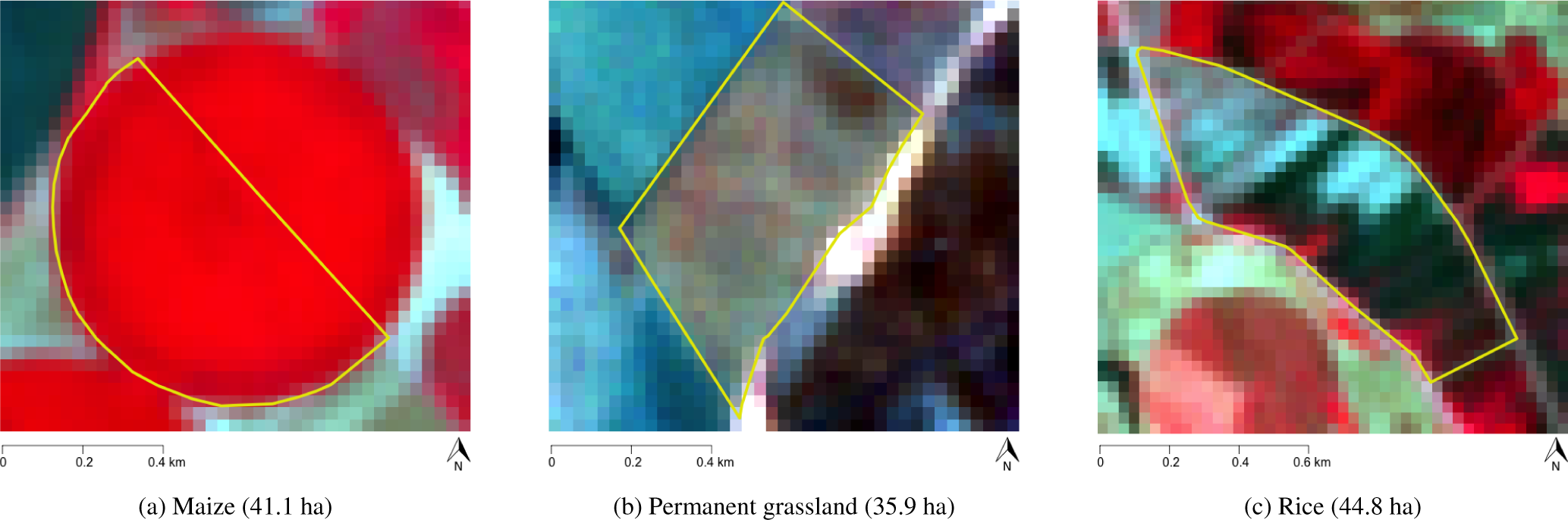
4.5. An Application Example

A practical application example is provided to illustrate how ACS works in the operational context. Classification results with two different reliability levels are discussed in this example: 80% and 95%. Figure 7 shows false color composites of three selected parcels with known land cover. The corresponding classification results can be found in

Table 6. Automatic classification results for the parcels represented in Figure 7. q_j values and corresponding results are with λ = 80% and λ = 95%.

Parcel	True Class	Classification Output		qj,80	qj,95	Result80	Result95
		Decision ωj	P(ωj|x)
(a)	MAI	MAI	0.950	0.239	0.439	Accepted	Accepted
(b)	PGL	FOR	0.647	0.686	0.831	Rejected	Rejected
(c)	RIC	MAI	0.389	0.239	0.439	Accepted	Rejected

.

Parcel (a) shows a homogeneous maize cropping with a very high spectral response. This led to a clear classification of the parcel as maize with a high posterior probability P(ω_j|x) of 0.95. This result was accepted for both reliability levels (λ = 80%, λ = 95%), and the parcel was classified automatically, since P(ω_j|x) was higher than both q_j(80%) and q_j(95%). Parcel (b) is covered by permanent grassland and shows a rather heterogeneous crop pattern. In the classification process, it was assigned to the incorrect class forage crops with posterior probability 0.647. However, the ACS correctly rejected that classification and decided not to classify the parcel in an automatic way, for both reliability levels. For 80% reliability, it was a close rejection, given that P(ω_j|x) almost matched the minimum of 0.686. As for 95%, the classification is clearly rejected, which makes sense, since demanding a higher reliability in the classification decisions increases the threshold to accept classifications, ultimately resulting in more rejected parcels. This parcel exemplifies the usefulness of the ACS, rejecting parcels that cannot be classified with the required certainty. The third example is Parcel (c), which corresponds to rice, revealing a very heterogeneous behavior. This parcel was also assigned to the wrong class by the classifier, in this case to maize, with an associated probability of 0.389. The low q_j for maize allows for misclassifications when parcels are classified as maize, even with relatively low posterior probabilities, which happened in this case. The classification was wrongly accepted by the system with a reliability level of 80% and correctly rejected with a reliability of 95%. This example clearly shows the positive effect a higher reliability level has on the accuracy of an automatic classification decision, with the drawback of automatically classifying a smaller proportion of the total number of parcels.

5. Conclusions

Every year, Common Agriculture Policy area-based subsidies are controlled using remote sensing imagery. This process, known by EU authorities as control with remote sensing, is done over each national Land Parcel Identification System. We used Portuguese official land parcels and an atmospherically-corrected Landsat 7 ETM+ time series to automatize crop identification for subsidy control. However, automatic classification of all parcels, as done in Blaes et al. [4], Matikainen et al. [13], Oesterle and Hahn [14], leads in our case to an overall accuracy of only 68%, which is explained by the similarities of the spectral characteristics of the crops relevant to agriculture subsidies. To address this problem, we coupled crop classification to a reliability requirement. This allows the decision-maker to set the reliability of the classifier, restricting automatic crop identification to parcels that are classified with high certainty. In this paper, we quantify the accuracy of the proposed approach and analyze the trade-off between the reliability level and the proportion of parcels that can be automatically controlled. Moreover, we estimate the proportion of land parcels, for 12 common agricultural occupations, that can be automatically classified.

When the reliability level increases from 50% to 100%, the overall proportion of parcels that are classified automatically decreases from 97.6% to 5.5%. In particular, our results suggest that with a reliability level of 80%, traditional photo interpretation of remote sensing imagery can be replaced by automatic crop identification for more than half of the parcels, with this proportion raising above 80% for maize, rice, wheat or vineyard. Furthermore, maize and rice were found to be easily identified, allowing us to control 100% of parcels with these classes in an automatic way. On the contrary, no parcels containing fallow, poor grassland and non-used area should be controlled due to extreme confusion between these classes. In our experiments, overall accuracy raised from 68% to 84% for that same 80% reliability level. Therefore, we have shown that automatic classification of agricultural land parcels can be reliably performed even when crops are difficult to discriminate.

As any other supervised classification methodology, the approach described in this paper requires a sample of land parcels with a known class for training and calibration. We foresee two ways of obtaining this in an operational context for each yearly subsidy control campaign. The first one would be to use the initial flow of photo-interpreted parcels for calibration and then partially replacing subsequent photo interpretation tasks, reducing the total number of parcels that would require non-automatic identification. Alternatively, one could use control data from a previous subsidy control campaign. However, this last procedure would require that remote sensing image acquisition dates for calibration and application to be similar. In this respect, we stress that the proposed methodology is conducive to multi-sensor analysis, since our results suggest that within-parcel variability is very low in comparison with between-parcel variability. This means that images with different resolutions can be combined in a single time series, since only the average reflectance for the parcel is used for classification. For instance, combining Landsat 7/8 data with images obtained from sensors, such as the upcoming Sentinel-2, would allow for the choice of images from a wider range of dates. This facilitates the selection of a time series that optimally follows the crops’ development cycle and helps to deal with missing data due to clouds or other constraints.

The 2014 CAP reform promotes crop diversification in the EU’s agriculture through the new “greening” policy instrument [1]. Therefore, a larger assortment of crops will have to be controlled by remote sensing. We believe this could be done more effectively by using methodologies like the one we describe in this paper.

References

- Singh, M.; Marchis, A.; Capri, E. Greening, new frontiers for research and employment in the agro-food sector. Sci. Total Environ. 2014, 472, 437–443. [Google Scholar]
- European Union. Regulation (EU) No. 1306/2013. Available online: http://eur-lex.europa.eu/LexUriServ/LexUriServ.do?uri=OJ:L:2013:347:0549:0607:EN:PDF accessed on 5 May 2015.
- Loudjani, P. G-tech supports a Common Agriculture Policy in Europe. Geosp. World 2013, 4, 38–40. [Google Scholar]
- Blaes, X.; Vanhalle, L.; Defourny, P. Efficiency of crop identification based on optical and SAR image time series. Remote Sens. Environ. 2005, 96, 352–365. [Google Scholar]
- Sagris, V.; Wojda, P.; Milenov, P.; Devos, W. The harmonised data model for assessing Land Parcel Identification Systems compliance with requirements of direct aid and agri-environmental schemes of the CAP. J. Environ. Manag. 2013, 118, 40–48. [Google Scholar]
- Castillejo-González, I.L.; López-Granados, F.; García-Ferrer, A.; Peña Barragán, J.M.; Jurado-Expósito, M.; de la Orden, M.S.; González-Audicana, M. Object-and pixel-based analysis for mapping crops and their agro-environmental associated measures using QuickBird imagery. Comput. Electron. Agric. 2009, 68, 207–215. [Google Scholar]
- Conrad, C.; Fritsch, S.; Zeidler, J.; Rücker, G.; Dech, S. Per-field irrigated crop classification in arid central Asia using SPOT and ASTER data. Remote Sens. 2010, 2, 1035–1056. [Google Scholar]
- Yang, C.; Everitt, J.H.; Murden, D. Evaluating high resolution SPOT 5 satellite imagery for crop identification. Comput. Electron. Agric. 2011, 75, 347–354. [Google Scholar]
- El Hajj, M.; Bégué, A. Guillaume, S.; Martiné, J.F. Integrating SPOT-5 time series, crop growth modeling and expert knowledge for monitoring agricultural practices—The case of sugarcane harvest on Reunion Island. Remote Sens. Environ. 2009, 113, 2052–2061. [Google Scholar]
- Peña Barragán, J.M.; Ngugi, M.K.; Plant, R.E.; Six, J. Object-based crop identification using multiple vegetation indices, textural features and crop phenology. Remote Sens. Environ. 2011, 115, 1301–1316. [Google Scholar]
- Blaschke, T. Object based image analysis for remote sensing. ISPRS J. Photogramm. Remote Sens. 2010, 65, 2–16. [Google Scholar]
- Sagris, V.; Devos, W. LPIS Core Conceptual Model: Methodology for Feature Catalogue and Application Schema; Joint Reaearch Centre of European Commission: Ispra, Italy, 2008. [Google Scholar]
- Matikainen, L.; Karila, K.; Litkey, P.; Ahokas, E.; Munck, A.; Karjalainen, M.; Hyyppä, J. The challenge of automated change detection: Developing a method for the updating of land parcels. ISPRS Ann. Photogramm. Remote Sens. Spat. Inf. Sci 2012, 1, 239–244. [Google Scholar]
- Oesterle, M.; Hahn, M. A case study for updating land parcel identification systems (IACS) by means of remote sensing, proceedings of the XX ISPRS Congress, Istanbul, Turkey, 13–22 July 2004.
- Carmona, V.M.P. The Role of Geographic Information Systems for the Control of Agricultural Subsidies in Portugal. Master’s Thesis, School of Agriculture, Lisbon, Portugal, 2012; In Portuguese. [Google Scholar]
- United States Geological Survey (USGS), Product Guide—Landsat Climate Data Record (CDR) Surface Reflectance; United States Geological Survey: Reston, VA, USA, 2014.
- Wardlow, B.D.; Egbert, S.L.; Kastens, J.H. Analysis of time-series MODIS 250 m vegetation index data for crop classification in the U.S. Central Great Plains. Remote Sens. Environ. 2007, 108, 290–310. [Google Scholar]
- Chander, G.; Markham, B.L.; Helder, D.L. Summary of current radiometric calibration coefficients for Landsat MSS, TM, ETM+, and EO-1 ALI sensors. Remote Sens. Environ. 2009, 113, 893–903. [Google Scholar]
- R Development Core Team, R: A Language and Environment for Statistical Computing; R Foundation for Statistical Computing: Vienna, Austria, 2014.
- Damodaran, B.B.; Nidamanuri, R.R. Assessment of the impact of dimensionality reduction methods on information classes and classifiers for hyperspectral image classification by multiple classifier system. Adv. Space Res. 2014, 53, 1720–1734. [Google Scholar]
- Jolliffe, I.T. Principal Component Analysis, 2nd ed.; Springer: New York, NY, USA, 2002. [Google Scholar]
- Duro, D.C.; Franklin, S.E.; Dubé, M.G. A comparison of pixel-based and object-based image analysis with selected machine learning algorithms for the classification of agricultural landscapes using SPOT-5 HRG imagery. Remote Sens. Environ. 2012, 118, 259–272. [Google Scholar]
- Peña, J.; Gutiérrez, P.; Hervás-Martínez, C.; Six, J.; Plant, R.; López-Granados, F. Object-based image classification of summer crops with machine learning methods. Remote Sens. 2014, 6, 5019–5041. [Google Scholar]
- Huang, C.; Song, K.; Kim, S.; Townshend, J.R.; Davis, P.; Masek, J.G.; Goward, S.N. Use of a dark object concept and support vector machines to automate forest cover change analysis. Remote Sens. Environ. 2008, 112, 970–985. [Google Scholar]
- Mountrakis, G.; Im, J.; Ogole, C. Support vector machines in remote sensing: A review. ISPRS J. Photogramm. Remote Sens. 2011, 66, 247–259. [Google Scholar]
- Lin, H.T.; Lin, C.J.; Weng, R.C. A note on Platt’s probabilistic outputs for support vector machines. Mach. Learn. 2007, 68, 267–276. [Google Scholar]
- Duda, R.O.; Hart, P.E.; Stork, D.G. Pattern Classification, 2nd ed.; John Wiley: New York, NY, USA, 2000; p. 680. [Google Scholar]
- Congalton, R.G. A review of assessing the accuracy of classifications of remotely sensed data. Remote Sens. Environ. 1991, 37, 35–46. [Google Scholar]