Theoretical Modeling and Analysis of L- and P-band Radar Backscatter Sensitivity to Soil Active Layer Dielectric Variations

Abstract

Freeze-thaw (FT) and moisture dynamics within the soil active layer are critical elements of boreal, arctic and alpine ecosystems, and environmental change assessments. We evaluated the potential for detecting dielectric changes within different soil layers using combined L- and P-band radar remote sensing as a prerequisite for detecting FT and moisture profile changes within the soil active layer. A two-layer scattering model was developed and validated for simulating radar responses from vertically inhomogeneous soil. The model simulations indicated that inhomogeneity in the soil dielectric profile contributes to both L- and P-band backscatter, but with greater P-band sensitivity at depth. The difference in L- and P-band responses to soil dielectric profile inhomogeneity appears suitable for detecting associated changes in soil active layer conditions. Additional evaluation using collocated airborne radar (AIRSAR) observations and in situ soil moisture measurements over alpine tundra indicates that combined L- and P-band SAR observations are sensitive to soil dielectric profile heterogeneity associated with variations in soil moisture and FT conditions.

1. Introduction

The Freeze-thaw (FT) state of vegetation and soil governs terrestrial water mobility and energy partitioning in boreal, arctic and alpine regions. These regions are characterized by widespread permafrost and seasonally frozen ground, where the solid or liquid state of water in the soil active layer is a major controlling factor for hydrologic and biological processes [1,2,3,4], with significant impacts on regional weather and climate [5,6]. Knowledge of FT and soil moisture characteristics is therefore essential for monitoring climate change impacts in FT affected regions. A number of parameters characterizing FT processes including the state of vegetation, soil active layer and associated timing, and duration of seasonal FT transitions, have important implications to high-latitude and alpine ecosystems. Studies focusing on the timing of FT transitions from long-term satellite microwave records in Alaska and the larger pan-boreal and Arctic domain indicate widespread earlier spring thawing and lengthening of the non-frozen season in recent years [7,8,9]. The degradation of permafrost associated with earlier and longer non-frozen seasons may promote further greenhouse gas emissions and global warming through enhanced decomposition of northern soil carbon stocks [10,11].

As the phase of water stored in soil, snow or vegetation changes between solid and liquid, the dielectric properties of these features show dynamic changes during the FT transition period. Microwave remote sensing, with its high sensitivity to surface dielectric changes associated with changes in relative abundance of liquid water in vegetation, snow and surface soil layers, has become one of the most viable tools for FT detection and monitoring over large regions [12,13]. Most studies on FT remote sensing are carried out using observations from space-borne radiometers or scatterometers at relatively high frequencies ranging from C-band to Ka-band. Such instruments include the Advanced Microwave Scanning Radiometer for EOS (AMSR-E) aboard the Aqua satellite, scatterometry from QuickScat and ASCAT sensors, and the future Surface Water and Ocean Topography (SWOT) radar [9,14,15]. In comparison with lower frequency (e.g., L-band) observations, microwave remote sensing at C-band or higher frequencies is more sensitive to upper layers of the vegetation canopy and surface snow cover conditions, where microwave scattering and attenuation are strongly affected by the scattering parameters within the volume, including scatter size, shape, spatial distribution, density and dielectric properties [16,17]. For soil FT retrievals, intervening vegetation and snow layers can be regarded as perturbing factors. In addition, limited soil penetration depth also constrains direct soil FT detection from microwave remote sensing at higher frequencies [18], since the microwave penetration depth is directly proportional to wavelength and inversely proportional to the root of the imaginary part of the medium permittivity [19]. In contrast, lower frequency sensors, including Phased Array type L-band Synthetic Aperture Radar (PALSAR), L-band Japanese Earth Resources Satellite-1 (JERS-1) SAR, S- band Huan Jing (HJ) SAR and Nova SAR-S, have improved penetration ability for soil FT detection and monitoring [20,21,22,23,24]. In particular, the NASA Soil Moisture Active and Passive (SMAP) mission [18] is expected to provide enhanced L-band sensitivity and reliable land surface FT state retrievals and operational products with moderate (3 km) spatial resolution, and global coverage every three days at the equator and two days at boreal latitudes (higher than 45 degrees North).

There are two limitations with the above FT mapping activities: (a) besides the upcoming L-band satellite missions, the FT measurements from current space-borne sensors are largely representative of surface vegetation canopy and snow conditions, with only secondary sensitivity to upper soil layer properties extending from the soil surface (0 cm) to a few centimeters depth, depending on vegetation surface and soil characteristics. At L-band frequencies, the theoretical penetration depth for frozen soil with a given dielectric constant of 3.6–0.9 j was estimated to be approximately 7.3 cm [25], while the penetration depth for non-frozen conditions is generally less than 5 cm [18]. (b) Most of the current FT mapping activities can be described as 2-Dimensional detection of the overall FT state of vegetation, snow cover (when present) and surface soil layer conditions within the sensor footprint. There is a general lack of soil FT profile information, which is greatly needed for soil active layer FT detection and monitoring, and for constraining climate, hydrology and ecosystem model predictions. To overcome these limitations, it is worthwhile to introduce lower frequency P-band SAR, in which the characteristic penetration depth is estimated to be several tens of centimeters even under moderately high soil moisture conditions, and with greater backscatter sensitivity to deeper soil layers than L-band [26]. Available P- band missions include the NASA Airborne Observatory of Subcanopy and Subsurface (AirMOSS) mission, which is equipped with a P-band (430 MHz) synthetic aperture radar (SAR) and seeks to improve estimates of North American net ecosystem carbon exchange (NEE) through high-resolution observations and estimation of surface to root zone (up to 1m depth) soil moisture [26,27]. Moreover, the European Space Agency’s (ESA) BIOMASS mission is under development and is expected to provide future global space-borne P-band SAR observations [28]. An important heritage instrument is the NASA Airborne Synthetic Aperture Radar (AIRSAR), which was capable of acquiring concurrent C-, L- and P-band observations. AIRSAR flew successful missions from 1988 to 2004, including airborne data acquisitions during the NASA Cold Land Processes Field Experiment (CLPX) [29], which provided valuable data for this study.

Both L- and P-band SAR can convey soil information under low to moderate vegetation biomass levels, but with characteristic variable depth sensitivities proportional to the different sensor frequencies. Therefore, the combination of L-band and P-band observations could enable potentially improved extraction of soil FT profile conditions and temporal dynamics. The objectives of this study were to (a) model and evaluate L- and P-band radar responses from layered soil; (b) evaluate the potential for detecting changes in the FT and moisture state of layered soil using combined L- and P-band radar observations, especially during the FT transition period. By exploiting the different penetration abilities and associated soil active layer depth sensitivities of the P- and L-band observations, the FT conditions of different vertical soil layers or in more general expression, the dielectric inhomogeneity of the soil profile, could be inferred.

2. Datasets

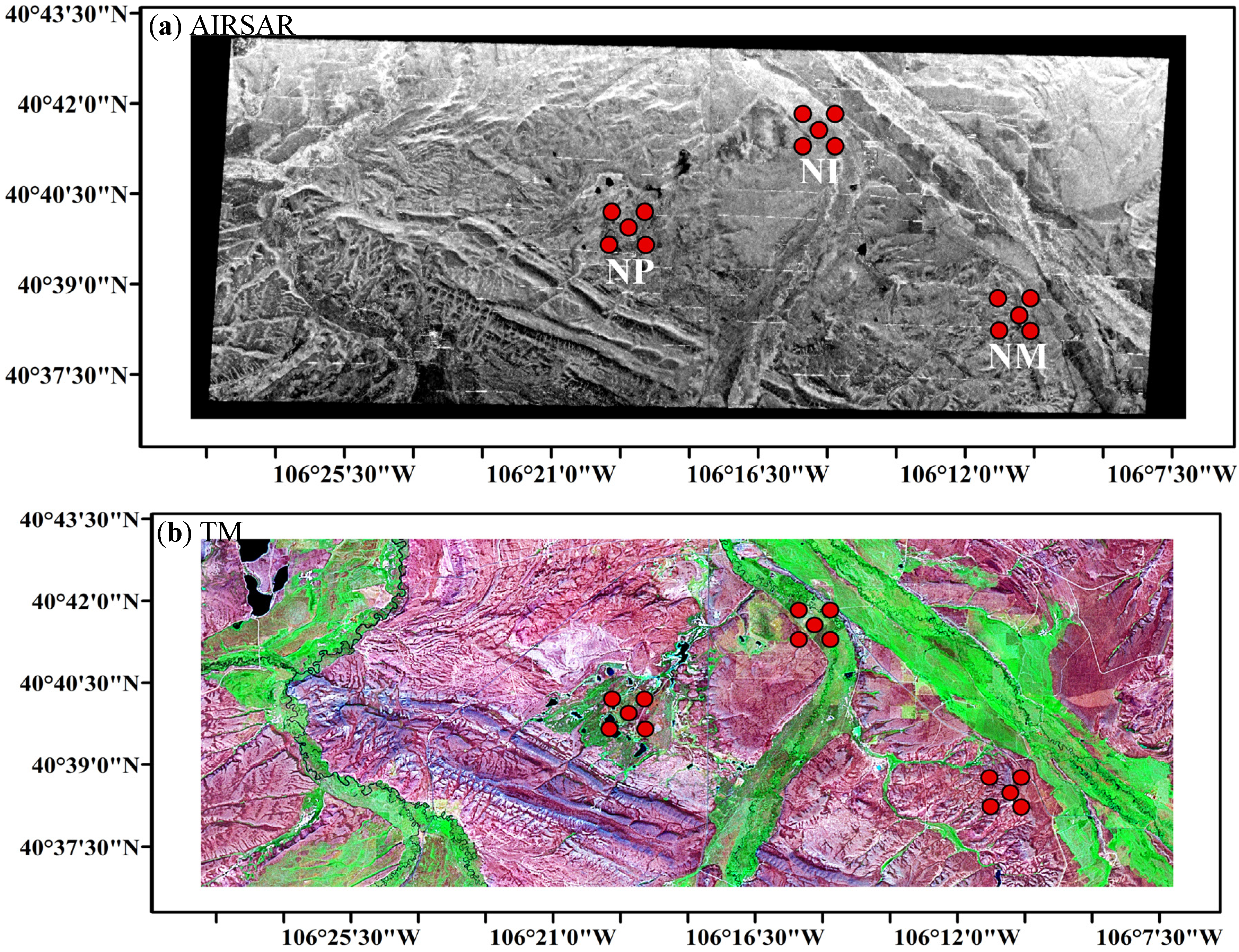
2.1. Field Experiment and Study Domain

AIRSAR fully polarimetric SAR (POLSAR) mode data coinciding with in situ meteorological station measurements acquired from the NASA Cold Land Processes Field Experiment (CLPX) were used in this study for evaluating L-band and P-band SAR sensitivity to soil active layer profile conditions over alpine tundra. CLPX was a multi-sensor, multi-scale experiment designed to develop quantitative understanding, models, and measurements necessary to extend local-scale understanding of water fluxes, storage, and transformations to regional and global scales [29]. During CLPX, data were collected during four intensive observation periods (IOPs) over North-Central Colorado, USA in February (IOP1) and March (IOP2) of 2002, and February (IOP3) and March (IOP4) of 2003. This study focuses on IOP4, when frozen and thawed, and dry and wet snow and surface soil conditions were widespread, and inhomogeneous dielectric properties in the upper soil layers were likely to be present. A 25 km × 25 km Meso-Cell Study Area (MSA) centrally located in North Park CO was selected as the primary domain for this investigation. North Park is a high elevation (mean elevation of 2499 m) alpine tundra region, characterized by low relief topography (total elevation range of 312 m), and sparse vegetation consisting mainly of shrubland and grassland suitable for radar soil measurements, while an extensive wetland complex is also located within the domain. Snow cover in this area tends to be shallow and windblown, typical of prairie and arctic- and alpine- tundra snow cover characteristics [29]. Surface soils (upper 5 cm) in the study area are predominantly sandy loam or loam [29].

Table 1. Locations of in situ measurement sites.

Site Name	Latitude (Degree)	Longitude (Degree)
NINW	40.700	−106.261
NINE	40.700	−106.249
NICT	40.696	−106.255
NISW	40.691	−106.260
NISE	40.691	−106.249
NPNE	40.672	−106.317
NPNW	40.672	−106.329
NPCT	40.668	−106.323
NPSW	40.663	−106.330
NPSE	40.663	−106.317
NMNW	40.650	−106.189
NMNE	40.650	−106.177
NMCT	40.645	−106.181
NMSW	40.641	−106.188
NMSE	40.641	−106.177

Table 1. Locations of in situ measurement sites.

Site Name	Latitude (Degree)	Longitude (Degree)
NINW	40.700	−106.261
NINE	40.700	−106.249
NICT	40.696	−106.255
NISW	40.691	−106.260
NISE	40.691	−106.249
NPNE	40.672	−106.317
NPNW	40.672	−106.329
NPCT	40.668	−106.323
NPSW	40.663	−106.330
NPSE	40.663	−106.317
NMNW	40.650	−106.189
NMNE	40.650	−106.177
NMCT	40.645	−106.181
NMSW	40.641	−106.188
NMSE	40.641	−106.177

In this study, we focused on 15 in situ measurement sites located inside three, 1 km × 1 km Intensive Study Areas (ISAs) nested within the larger North Park MSA, and identified as the Michigan River (NM), Illinois River (NI), and Potter Creek (NP) ISAs. The parameters measured during CLPX IOP4 include snow depth, air temperature, soil temperature and moisture at three depths (5 cm, 20 cm and 50 cm) [29,30,31]. The site locations (listed in Table 1) are denoted in Figure 1. Among all sites, NICT, NPCT and NMCT lie approximately in the center of the three ISAs while the other sites are located near the four corners of the ISAs.

2.2. In Situ Measurements

Systematic measurements of snow, air and soil parameters within the ISAs were made during CLPX IOP4 [29,30,31]. According to the two datasets, ISA Corner Site Meteorological Data and ISA Main Meteorological Data [30], air temperatures at site NICT, NPCT, and NMCT were colder than −5 °C while soil temperatures at 5- cm and 20- cm depths were slightly warmer than 0 °C ( about 0.4 °C to 0.99 °C). Similar to soil temperature, soil moisture measurements from most of the 15 sites indicated thawed or partially thawed soil conditions (volumetric soil moisture ranging from 0.05 cm³/cm³ to 0.40 cm³/cm³), except for the NPCT site where very low soil moisture levels (0.037 cm³/cm³) were observed at 5 cm depth. In addition, shallow snow depths ranging from 5.5 cm to 35.5 cm were also recorded at the 15 sites. There were no snow wetness measurements specifically taken at these sites, but periodic snow pit measurements [31] taken throughout the North Park MSA indicated dry to moist snow pack conditions over the IOP4 campaign. In addition, according to the snow pit measurements, there was only sparse vegetation in some parts of the MSA, while other MSA areas indicate the presence of grass or sage vegetation. Based on the above measurements, the study sites can be characterized as sparse and frozen vegetation, dry or moist shallow snow and layered soil which was thawed or partially thawed.

Figure 1. (a) HH Polarized L-band AIRSAR Georeferenced image (CM6608) and (b) TM band 7, 4, 2 color composite image acquired during September 2001 over the North Park Mesoscale Study Area (MSA); red circles denote locations of the 15 in situ soil moisture and temperature measurement sites. The labels NI, NP and NM represent three Intensive Study Areas (ISAs) inside the North Park MSA, denoted as Illinois River, Potter Creek and Michigan River, respectively.

Figure 1. (a) HH Polarized L-band AIRSAR Georeferenced image (CM6608) and (b) TM band 7, 4, 2 color composite image acquired during September 2001 over the North Park Mesoscale Study Area (MSA); red circles denote locations of the 15 in situ soil moisture and temperature measurement sites. The labels NI, NP and NM represent three Intensive Study Areas (ISAs) inside the North Park MSA, denoted as Illinois River, Potter Creek and Michigan River, respectively.

2.3. Radar Imagery

The Airborne Synthetic Aperture Radar (AIRSAR) sensor was a side-looking imaging radar flown on the NASA DC-8 aircraft. During CLPX, AIRSAR in POLSAR mode provided fully polarimetric measurements at 0.43 GHz (P-band), 1.26 GHz (L-band), and 5.31 GHz (C-band) over the three MSAs at Rabbit Ears, North Park, and Fraser [29,32]. The flights were conducted in IOP1, IOP2, September 2002 and IOP4. The AIRSAR–POLSAR images were processed and calibrated by the Jet Propulsion Laboratory (JPL). The POLSAR data stored in the compressed Stokes matrix files have a nominal pixel spacing of 9.26 m (along-track direction) and 3.3 m (cross-track direction), and remain in the natural SAR slant-range projection. In this study, initial quality control was conducted on the AIRSAR images by examining frequency and polarization relationships of the radar backscatter data. The images were considered unacceptable for this study if: (a) the average HH-polarized backscatter was significantly higher than the VV-polarization data (3-dB at approximately 40° incident angle for this study) over bare soil or sparsely vegetated areas, since this is contradictory to what theory predicts [33]; (b) P-band backscatter was significantly lower than L-band for the same polarization (10-dB at approximately 40° incident angle for this study) since this is inconsistent with the theoretical simulations in Section 4.4. Based on the above criteria, AIRSAR images (CM6608 and CM6610) acquired 28 March 2003 were selected and further processed in ENVI with the following steps: slant to ground range projection Georeferencing using image corner coordinates from overlapping Landsat Thematic Mapper (TM) imagery, and speckle filtering by performing a 9 × 9 pixel moving average window. The incidence angles of image CM6608 and CM6610 range from 28.0° to 64.2°. The swath width in the cross-track direction is 8.3 km and the length of the processed line is 30.3 km. The resulting image is in Universal Transverse Mercator (UMT) projection with a spatial resolution of 14.25 m, and consistent with the TM image used in the image registration. Considering the low relief of the North Park MSA, no terrain correction was applied to the SAR images. After processing, collocated AIRSAR backscatter with incidence angles ranging from 38° to 60° and in situ soil moisture, temperature and snow depth measurements for the 15 study sites (Table 1) within the North Park MSA were extracted; all 15 study sites were within CM6608, while only 10 points from NP and NM ISAs were covered by CM6610. A sample of the georeferenced AIRSAR HH dB image from CM6608 along with the TM image for the same area is shown in Figure 1.

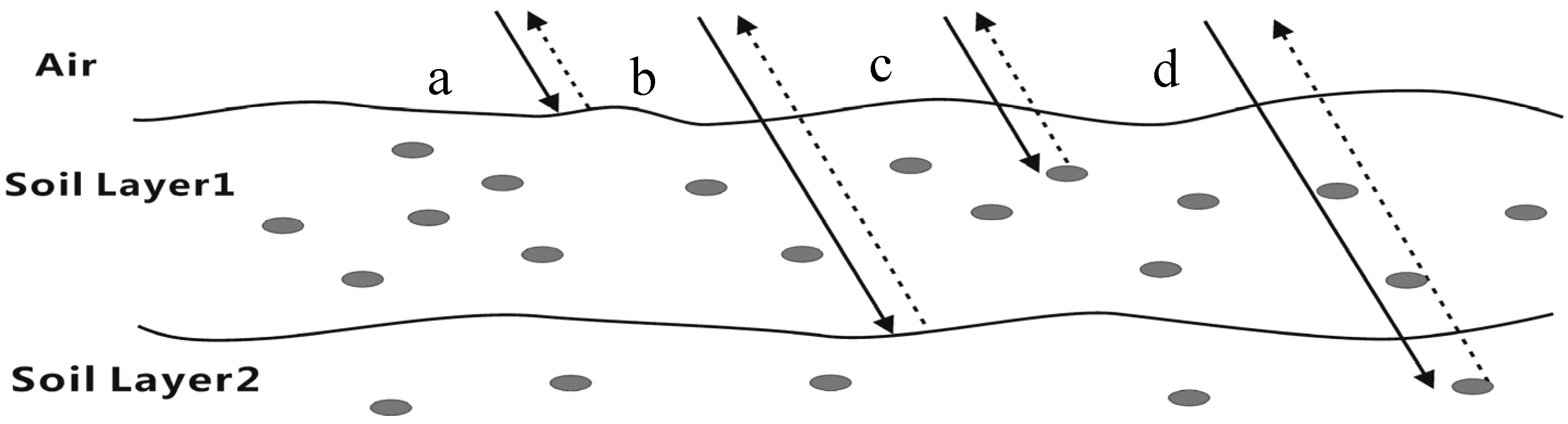
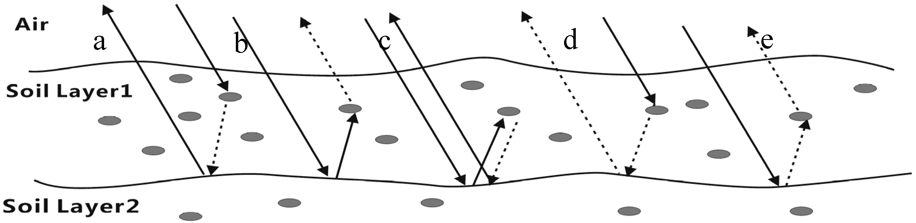
3. Theoretical Modeling

In the soil active layer, the frost depth generally increases (decreases) as surface air temperature decreases (increases) during the FT transition period. Previous studies based on multi-temporal L-band radiometer observations demonstrate the potential of retrieving the penetration velocity of the frost front within the soil active layer [34]. With additional P-band sensor observations, the progressive thawing or freezing process and associated change in soil liquid water content are more likely to be captured and characterized. For this purpose, a two-layer soil scattering (FTSS) model is developed for L- and P-band microwave observations based on first-order solution of the Radiative Transfer Equation. The soil dielectric profile during the FT transition period can be described by a Fermi-distribution function and dielectric constants for frozen and unfrozen conditions of relatively moist soils [34]. As a simplification, we separate the soil profile into two adjacent layers, representing predominantly frozen and thawed conditions. The soil vertical inhomogeneity is therefore represented by two discrete soil layers with significant dielectric contrast associated with the different FT conditions.

The total radar backscatter from the two-layer soil is mainly contributed from the following five surface scattering mechanisms: (a) σ_s1, scattering from the first layer surface or air-soil interface; (b) σ_s2, scattering from the upper surface of the second layer or first-second layer interface. The scattering is caused by the dielectric contrast between the two layers and is attenuated by the first layer; (c) σ_v1, volume scattering inside the first layer; (d) σ_l12, interactions between first and second soil layers; and (e) σ_v2, volume scattering in the second soil layer attenuated by the first layer. To calculate direct backscattering and bi-static scattering from the surface, the Advanced Integral Equation Method (AIEM) [33] was implemented in the model. Similar to [35], in which soil clods are deemed as dominant scatters and modeled as deformed ellipses, we modeled soil scatters as ellipsoids with short to long axis ratio 0.8. Rayleigh Approximation [36] was applied to the ellipsoid particles to calculate the phase matrix of the soil layer. The soil dielectric model in [37] is adopted in this study. The mathematical expressions of σ_s1, σ_s2 and σ_v1 are given in the following equations [38].

$${\text{σ}}_{s1}=S_{01}({\text{θ}}_i,\text{π}+{\text{ϕ}}_i;{\text{θ}}_i,{\text{ϕ}}_i)$$

(1)

$${\text{σ}}_{s2}=T_{10}({\text{θ}}_{i1})S_{12}({\text{θ}}_{i1},\text{π}+{\text{ϕ}}_i;{\text{θ}}_{i1},{\text{ϕ}}_i)\exp \left[-2{\text{κ}}_{e1}{d}_1/\cos ({\text{θ}}_{i1})\right]T_{01}({\text{θ}}_i)$$

(2)

$${\text{σ}}_{v1}=T_{10}({\text{θ}}_{i1})P_1({\text{θ}}_{i1},\text{π}+{\text{ϕ}}_i;{\text{θ}}_{i1},{\text{ϕ}}_i)\frac{1-\exp (-2k_{e1}d/\cos ({\text{θ}}_{i1}))}{(2/\cos ({\text{θ}}_{i1}))k_{e1}}{T}_{01}({\text{θ}}_i)$$

(3)

where S is the phase matrix of the surface, P is the phase matrix of the soil medium, T is the transmissivity matrix, d is the depth of the soil layer, K_e is the microwave extinction coefficient, θ_i is the incident angle of radar measurement, ϕ_i is the azimuth angle of incident direction of measurement and the subscripts (0, 1, 2) denote air, first soil layer and second soil layer, respectively. σ_v2 has a similar expression as Equation (3) but with additional attenuation from layer 1. σ_s1, σ_s2, σ_v1 and σ_v2 are also illustrated in Figure 2.

Figure 2. Representation of the major radar scattering mechanisms (except for interactions between layers) from a two-layer soil, including (a) scattering from the air-soil interface; (b) scattering from the first-second layer interface; (c) volume scattering inside the first layer, and (d) volume scattering in the second soil layer attenuated by the first layer; soil clods are assumed to be dominant scatterers and depicted as oblong ellipsoids (in gray).

Figure 2. Representation of the major radar scattering mechanisms (except for interactions between layers) from a two-layer soil, including (a) scattering from the air-soil interface; (b) scattering from the first-second layer interface; (c) volume scattering inside the first layer, and (d) volume scattering in the second soil layer attenuated by the first layer; soil clods are assumed to be dominant scatterers and depicted as oblong ellipsoids (in gray).

The term σ_l12 actually consists of five interaction components, which are (a) downward scattering by the first layer soil particles or air-soil interface, followed by coherent scattering by the first-second soil layer interface; (b) coherent scattering by the first-second soil layer interface, followed by incoherent scattering from particles inside the first soil layer or air-soil interface; (c) coherent scattering by the first- second layer soil interface, followed by particle scattering in the first soil layer and coherent scattering of the first-second layer interface; (d) particle scattering in the first soil layer or air-soil interface followed by non-coherent scattering by the first-second layer interface; (e) non-coherent scattering by the first-second layer interface followed by scattering from the particles in the first soil layer or air-soil interface. The detailed expression of term σ_l12 is provided elsewhere [16,38], while the interaction components are illustrated in Figure 3.

Figure 3. Representation of Radar backscatter interactions between soil layers, including downward scattering by soil particles (in gray) in the first layer or air-soil interface, (a) followed by coherent scattering from the first-second soil layer interface; coherent scattering by the first-second soil layer interface, (b) followed by incoherent scattering from particles inside the first layer or air-soil interface; coherent scattering by the first-second soil layer interface, (c) followed by particle scattering in the first layer and coherent scattering from the first-second layer interface; particle scattering in the first layer or air-soil interface, (d) followed by non-coherent scattering from the first-second soil layer interface; non-coherent scattering by the first-second soil layer interface, (e) followed by scattering from particles in the first layer or air-soil interface.

Figure 3. Representation of Radar backscatter interactions between soil layers, including downward scattering by soil particles (in gray) in the first layer or air-soil interface, (a) followed by coherent scattering from the first-second soil layer interface; coherent scattering by the first-second soil layer interface, (b) followed by incoherent scattering from particles inside the first layer or air-soil interface; coherent scattering by the first-second soil layer interface, (c) followed by particle scattering in the first layer and coherent scattering from the first-second layer interface; particle scattering in the first layer or air-soil interface, (d) followed by non-coherent scattering from the first-second soil layer interface; non-coherent scattering by the first-second soil layer interface, (e) followed by scattering from particles in the first layer or air-soil interface.

4. Results and Discussion

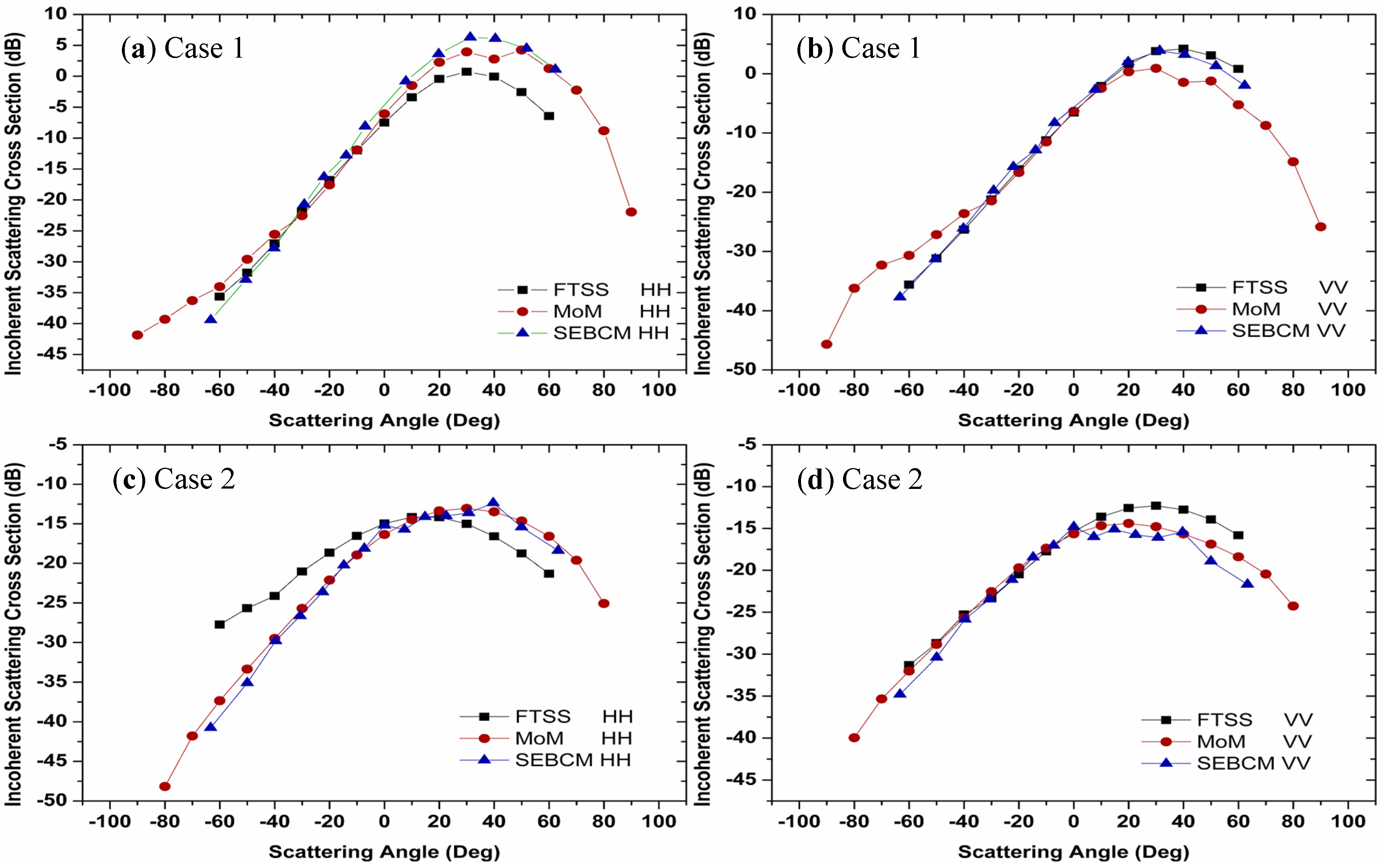
4.1. Model Comparisons

Microwave scattering from a multi-layer medium has been studied based on different approaches including the classical extended boundary condition method (EBCM) [39], Kirchhoff approximation [40], and small perturbation method [41]. As a recent development, the scattering problem was modeled by the scattering matrix approach and the stabilized extended boundary condition method (SEBCM) developed for multilayer rough surfaces within homogeneous or inhomogeneous media [42]. The multilayer SEBCM was shown to have good agreement with the rigid numerical approach of the method of moments (MoM). Alternatively, the proposed AIEM-based first-order scattering model considers a number of scattering mechanisms, including surface scattering and volume scattering. The FTSS model used for the current study has the capability of separating the contribution of each mechanism from the total backscatter signal, which is especially helpful in understanding the scattering problem for soil media with vertical dielectric variations. For validation purposes, the FTSS model simulations are compared against SEBCM and MoM results determined using the same input parameters adopted from [42] and also listed in Table 2. In the Table 2 summary of model inputs, Case 1 represents rough surface conditions and Case 2 represents smooth surface conditions.

Model inter-comparison results for Cases 1 and 2 are plotted in Figure 4. The results show that for both surface roughness conditions, the FTSS method is largely consistent with both SEBCM and MoM for moderate and small scattering angles ranging from −40° to 40°. In particular, the FTSS and MoM backscatter results show favorable agreement for all simulations. This is expected, since FTSS is based on the AIEM model, which was verified by laboratory measurements of bistatic scattering from surfaces with small, intermediate and large scale roughness [33]. As for large scattering angles, relatively large discrepancies are found between the FTSS and MoM simulations for HH polarization in Case 2. These results indicate that the FTSS approach is especially suitable for simulating radar backscattering for a layered medium.

Table 2. Input parameters for model simulations; k is the free space wavenumber, $\text{λ}$ is wavelength, h and l are the surface Root Mean Square (RMS) height and Correlation length, respectively. Sensing incident angle is fixed at 40°.

Case 1
Parameter	First layer	Second layer
kh	π/5	π/10
Kl	2 π	π
Dielectric constant	5.4 + 0.44i	11.27 + i
Depth	0.8λ	N/A
Correlation function	Gaussian
Case 2
kh	π/25	π/25
Kl	π	π
Dielectric constant	5.4 + 0.44i	11.27 + i
Depth	λ / 5	N/A
Correlation function	Gaussian

Table 2. Input parameters for model simulations; k is the free space wavenumber, $\text{λ}$ is wavelength, h and l are the surface Root Mean Square (RMS) height and Correlation length, respectively. Sensing incident angle is fixed at 40°.

Case 1
Parameter	First layer	Second layer
kh	π/5	π/10
Kl	2 π	π
Dielectric constant	5.4 + 0.44i	11.27 + i
Depth	0.8λ	N/A
Correlation function	Gaussian
Case 2
kh	π/25	π/25
Kl	π	π
Dielectric constant	5.4 + 0.44i	11.27 + i
Depth	λ / 5	N/A
Correlation function	Gaussian

Figure 4. Comparison of incoherent scattering cross sections derived from FTSS, SEBCM, and MoM at 40° incident angle for a two-layer medium using model parameters summarized in Table 2 as Case 1 (a,b) and Case 2 (c,d).

Figure 4. Comparison of incoherent scattering cross sections derived from FTSS, SEBCM, and MoM at 40° incident angle for a two-layer medium using model parameters summarized in Table 2 as Case 1 (a,b) and Case 2 (c,d).

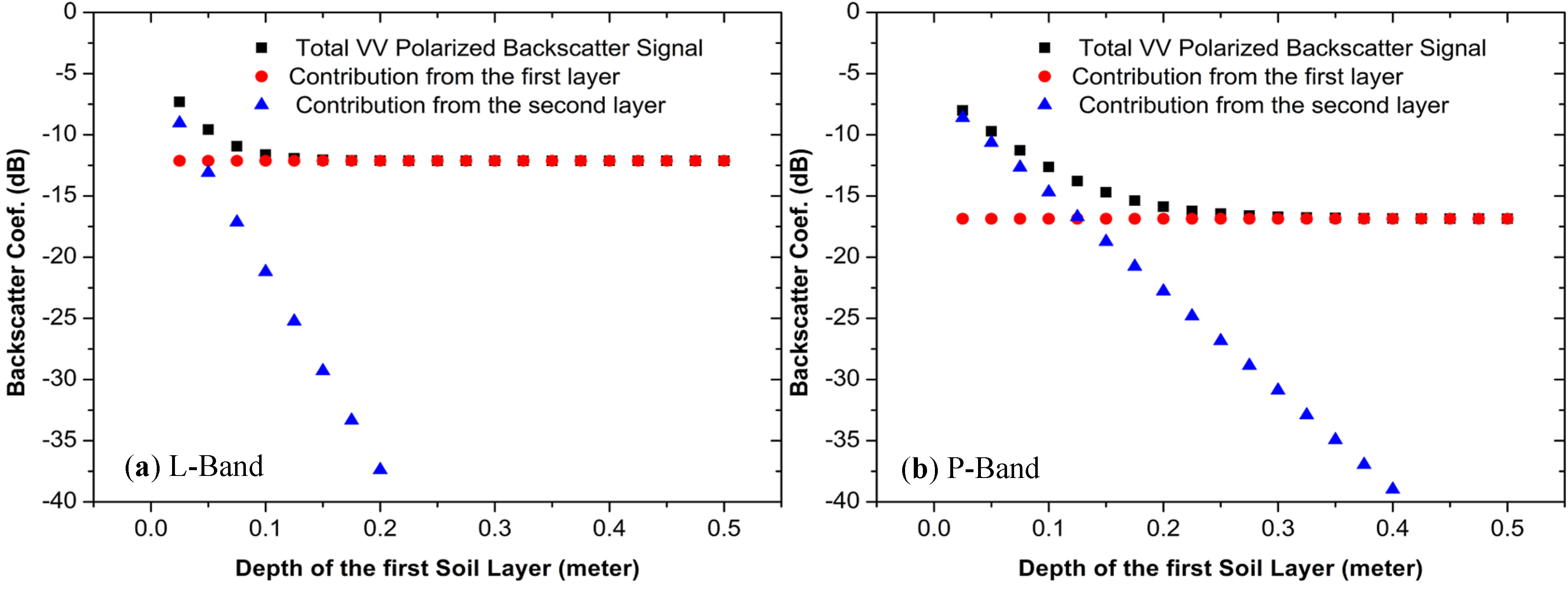
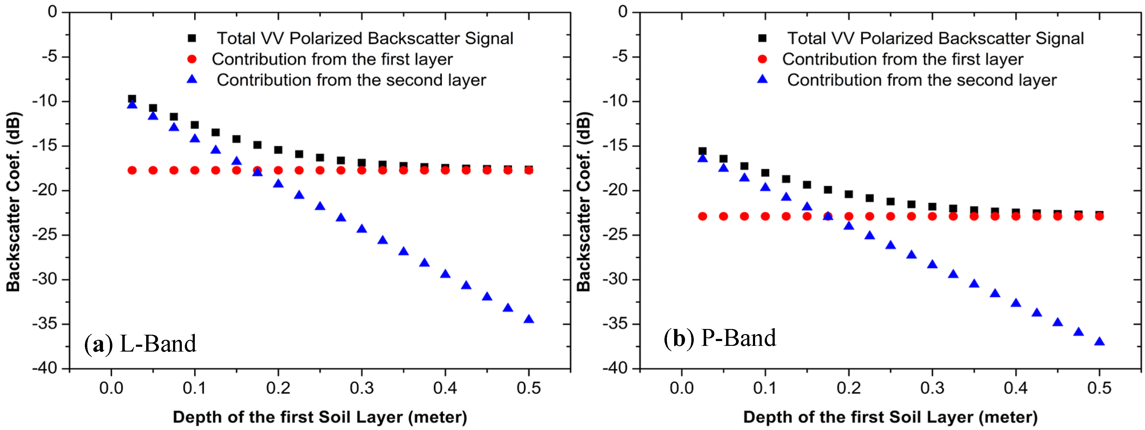
4.2. Effects of Soil Volume Scattering

The effects of soil volume scattering on radar or radiometer measurements at C-band or higher frequencies have been observed and modeled in a few studies [35,43]. The lower frequency L- and P-band observations, relative to C- and X-band, have deeper soil penetration depth and smaller volume scattering effects. It is interesting to evaluate soil volume scattering effects for these two frequencies, especially for dry or frozen soil when volume scattering becomes more important [35,43]. For this purpose, we make a similar assumption as [35] that the soil medium is composed of fine earth and large soil particles, which are the primary elements of soil volume scattering. Based on the FTSS, we evaluated soil volume scattering effects by considering one deep frozen layer with ellipsoid soil particles of varying sizes. The detailed model input parameters and simulation results are listed in Table 3.

Table 3. Model input parameters and simulation results for studying soil volume scattering effects.

L-Band (1.26 GHz)
	VV (dB)	HH (dB)	VH (dB)	HV (dB)	Particle Diameter (mm)
σs1	−14.9	−17.1	−31.8	−31.8
σv1	−41.6	−43.4	−68.4	−68.4	5
σv1	−27.3	−29.1	−54.1	−54.1	15
σv1	−18.4	−20.2	−45.2	−45.2	30
P-Band (0.43 GHz)
σs1	−20.1	−24.1	−39.7	−39.7
σv1	−59.0	−60.8	−85.7	−85.7	5
σv1	−44.6	−46.4	−71.4	−71.4	15
σv1	−35.6	−37.4	−62.4	−62.4	30

Notes: Model input parameters also include layer depth 0.5 m; scatter volume fraction 26%; relative permittivity of the layer 6.7; relative permittivity of soil particle 8.5; air-soil interface RMS height 1.5 cm, correlation length 15 cm; and incident angle 40°.

Table 3. Model input parameters and simulation results for studying soil volume scattering effects.

L-Band (1.26 GHz)
	VV (dB)	HH (dB)	VH (dB)	HV (dB)	Particle Diameter (mm)
σs1	−14.9	−17.1	−31.8	−31.8
σv1	−41.6	−43.4	−68.4	−68.4	5
σv1	−27.3	−29.1	−54.1	−54.1	15
σv1	−18.4	−20.2	−45.2	−45.2	30
P-Band (0.43 GHz)
σs1	−20.1	−24.1	−39.7	−39.7
σv1	−59.0	−60.8	−85.7	−85.7	5
σv1	−44.6	−46.4	−71.4	−71.4	15
σv1	−35.6	−37.4	−62.4	−62.4	30

Notes: Model input parameters also include layer depth 0.5 m; scatter volume fraction 26%; relative permittivity of the layer 6.7; relative permittivity of soil particle 8.5; air-soil interface RMS height 1.5 cm, correlation length 15 cm; and incident angle 40°.

Parameters such as soil clod size, volume fraction and dielectric properties are described in [35]. As the diameter of the equivalent soil particle sphere increases from 5 mm to 15 mm, the volume backscattering at L-band VV polarization increases from a negligibly small value of −41.6 dB to −27.3 dB, which is still much lower than the direct backscatter (about −14.9 dB) from the air-soil interface. Similar results are found for L-band HH polarization backscatter. For cross-polarized signals at L-band and all channels at P-band, volume scattering is very small compared with surface scattering. The only exceptions are found for extremely large soil particles with average sizes reaching 30 mm in diameter; co-polarized volume scattering at L-band (about −18.4 dB for VV polarization) can also be comparable to the surface backscatter. Therefore, the simulations suggest that volume scattering can be generally ignored in analyzing P-band and most L-band radar observations of frozen or dry soil unless the majority of soil particles consist of large gravels or coarse grains approaching or exceeding 30 mm in diameter. Based on these results, no volume scattering is considered in the following (sub) sections.

4.3. Effects of Soil Profile Heterogeneity

At higher latitudes and elevations, the soil is strongly affected by FT events at both seasonal and diurnal time scales. The soil dielectric profile, which is governed by soil texture, ice and water content, can show complex spatial and vertical profile patterns, especially during the FT transition period. Based on the FTSS model, theoretical analysis of simulated L- and P-band backscatter responses to layered soil with vertical dielectric variations was performed to evaluate the potential for monitoring soil profile FT and moisture variations using combined L- and P-band SAR remote sensing. Two typical cases describing the layered soil during the FT transition period are considered in the following simulations: (a) wet-dry case: a thawed upper layer with volumetric soil moisture (VSM 35%) and a frozen lower layer (VSM 5%); (b) dry-wet case: a frozen/refrozen upper soil layer (VSM 5%) and a thawed lower layer (VSM 35%). For air-soil and first-second layer surfaces, the RMS height values are assumed to be 1.5 cm and 1.0 cm, with correlation lengths of 15 cm and 10 cm, respectively. Simulations were performed at a 40° incident angle with different first layer depths for both L-band (1.26 GHz) and P-band (435 MHz) frequencies. A changing first-layer depth in the simulation is used as a simple way to represent the vertical progression of a FT event through the soil profile. The simulation results, including both total backscatter and the contributions from each soil layer, were plotted in Figure 5 and Figure 6 for the wet-dry case and dry-wet case, respectively.

As is seen in Figure 5 for the wet-dry case, the contributions from both the first and second soil layers are important to L- and P-band radar backscatter observations when a very shallow (<5 cm) thawed soil layer is present. A strong contribution from the second soil layer is expected since (a) the incident angle becomes steeper after entering the wet soil with high dielectric constant from air as described by Snell’s Law, and (b) high contrast in dielectric constants between the first and second soil layers is present. As the wave progresses into deeper soil, the importance of subsurface frozen soil is quickly diminished for L-band, but still plays an important role for the P-band observations until the first-layer soil depth is deeper than approximately 20 cm. After the first-layer depth exceeds 20 cm, most of the signal from the second soil layer is attenuated by the wet first layer and the total radar backscatter becomes relatively stable and insensitive to thaw depth. Thus, at the beginning of the thaw process both L- and P-band radars sense the soil profile heterogeneity, but to different extents; whereas when soil thawing progresses to deeper soil layers, both microwave frequencies see a homogeneous soil within their effective penetration ranges.

Figure 5. Total radar backscatter and associated dB contributions from different soil layers with varying first-layer soil depths for VV polarization at (a) L-band and (b) P-band simulated by the FTSS model (wet-dry case with VWC 35% for the first layer and 5% for the second layer, respectively).

Figure 5. Total radar backscatter and associated dB contributions from different soil layers with varying first-layer soil depths for VV polarization at (a) L-band and (b) P-band simulated by the FTSS model (wet-dry case with VWC 35% for the first layer and 5% for the second layer, respectively).

Similarly, the L- and P-band radar backscatter responses to freezing (dry-wet case) are presented in Figure 6. Due to the weak attenuation of the frozen upper soil layer, the contribution from the underlying wet soil persists until the freezing depth reaches approximately 25 cm for L-band and 30 cm for P-band. When soil freezing extends below 35 cm depth, both frequencies see homogeneous frozen soil.

Figure 6. Total backscatter and associated dB contributions from different soil layers with varying first-layer depth for VV polarization at (a) L-band and (b) P-band simulated by the FTSS model (dry-wet case with VWC 5% for the first layer and 35% for the second layer, respectively).

Figure 6. Total backscatter and associated dB contributions from different soil layers with varying first-layer depth for VV polarization at (a) L-band and (b) P-band simulated by the FTSS model (dry-wet case with VWC 5% for the first layer and 35% for the second layer, respectively).

Based on the above analyses, it can be generalized that (a) total backscatter consists of contributions from different soil layers; therefore, vertical inhomogeneity of the soil dielectric profile generally leads to enhanced radar backscatter signals than the case when only a homogenous upper soil layer is considered; (b) the soil dielectric contrast at shallow soil profile depths is generally more measureable or contributes more to the radar backscatter observations than that of deeper soil depths; (c) due to different inherent penetration capabilities, inhomogeneity in the soil dielectric profile generally contributes more to P-band observations than L-band.

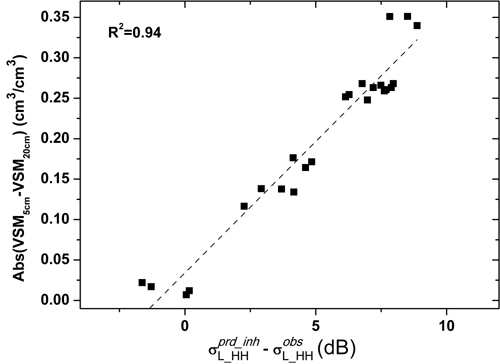
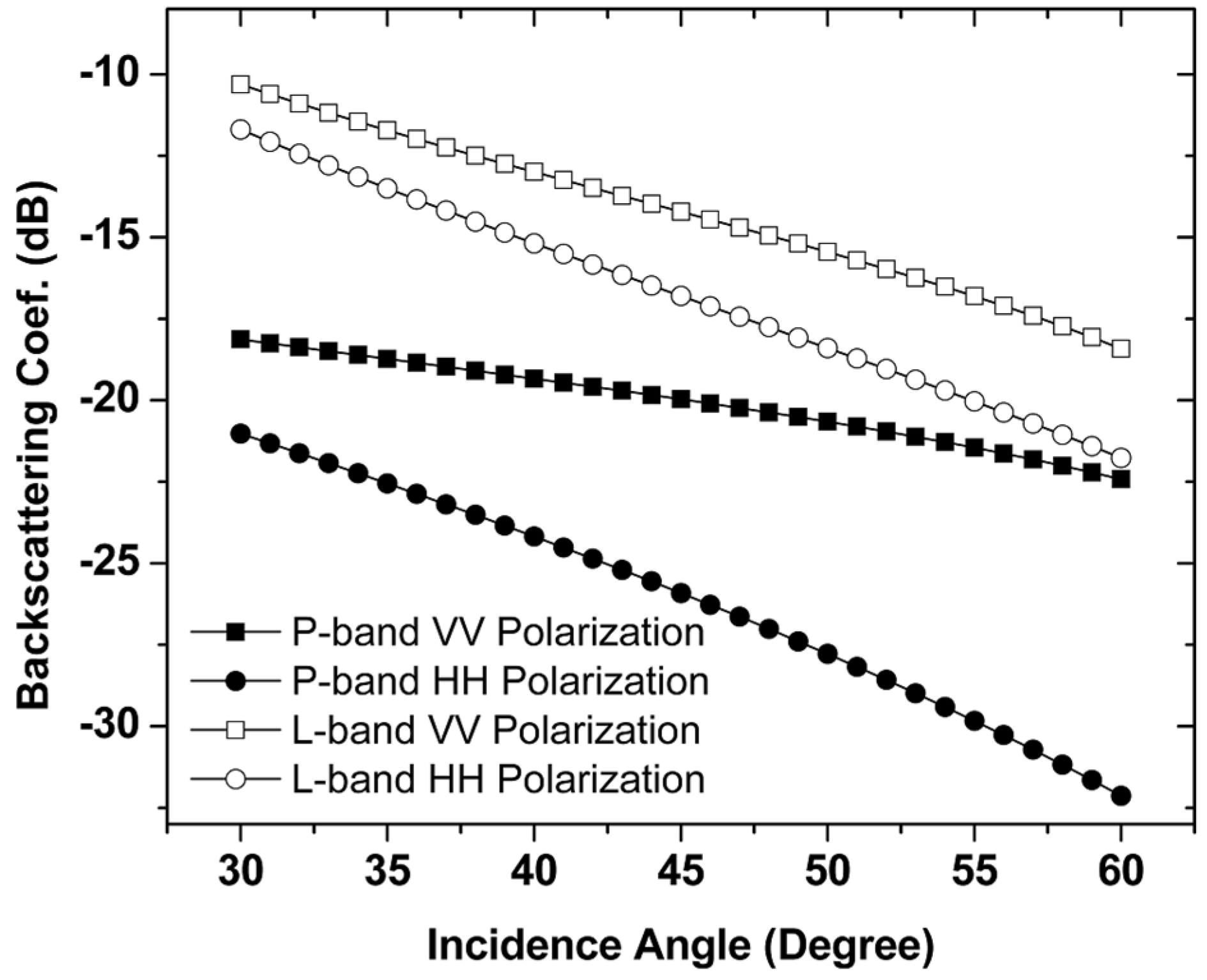
4.4. Detection of Soil Dielectric Profile Inhomogeneity Using AIRSAR

The theoretical analyses summarized in Section 4.3 demonstrates the potential for combined L- and P-band SAR detection of soil profile heterogeneity and monitoring of active layer FT and moisture changes by exploiting the different characteristic penetration depths and varying soil layer sensitivities of the two microwave frequencies. The CLPX AIRSAR acquisitions over North Park CO are used as a case study for alpine tundra to investigate the potential for L- and P-band SAR retrieval of soil profile heterogeneity similar to the theoretical analysis. In the following subsections, a simple method to detect soil profile heterogeneity with combined L- and P-band AIRSAR observations was developed in three steps, (a–c). The method was then applied to the AIRSAR observations from CLPX IOP4 and validated against in situ soil profile measurements as described in subsection (d) below.

(a) Correction of angular effects in AIRSAR observations for homogenous soil

In order to apply the proposed technique to AIRSAR observations with variant incidence angles, angular effects need to be corrected first to ensure all the analyses are based on the same viewing geometry. As summarized in [44], incidence angle normalization techniques include the classic cosine correction, radiative transfer-based models and statistics-based methods. In this study, theoretical relationships between radar backscatter from homogenous soil and a single soil surface at different incident angles were established based on simulations from the AIEM model [45], considering a variety of surface roughness and soil moisture conditions summarized in Table 4. In addition, the following analyses were limited to conditions where L-band HH-polarized backscatter at 40° is larger than −25 dB, excluding extreme cases representing approximately 8.6% the simulation database. An example of the simulated backscatter angular response was is shown in Figure 7.

Table 4. Input parameters for the AIEM simulation database.

	From	To	Interval
Incidence Angle	30°	60°	1°
RMS height	0.5 cm	3.0 cm	0.25 cm
Correlation Length	5 cm	25 cm	2.5 cm
Volumetric Soil Moisture	0.05 m3/m3	0.45 m3/m3	0.025 m3/m3
Frequencies: L-band (1.26 GHz) and P-band (0.43 GHz); Exponential Correlation Function

Table 4. Input parameters for the AIEM simulation database.

	From	To	Interval
Incidence Angle	30°	60°	1°
RMS height	0.5 cm	3.0 cm	0.25 cm
Correlation Length	5 cm	25 cm	2.5 cm
Volumetric Soil Moisture	0.05 m3/m3	0.45 m3/m3	0.025 m3/m3
Frequencies: L-band (1.26 GHz) and P-band (0.43 GHz); Exponential Correlation Function

Figure 7. Radar backscatter angular responses for L- and P-band frequencies based on AIEM simulations with the following input parameters: RMS height 1.25 cm, correlation length 10 cm, volumetric soil moisture 0.25 cm³/cm³ and exponential correlation function.

Figure 7. Radar backscatter angular responses for L- and P-band frequencies based on AIEM simulations with the following input parameters: RMS height 1.25 cm, correlation length 10 cm, volumetric soil moisture 0.25 cm³/cm³ and exponential correlation function.

Based on the simulation database, it was found that the backscatter at different incidence angles for either L- and or P-band are highly linearly correlated, with a coefficient of determination (R²) above 0.98. The angular relationship between radar backscatter at a given incident angle θ measured in radians and that at a reference incidence angle 40/180 π radians is established as shown in Equation (4) and illustrated in Figure 8. Each incident angle in the simulation database can be used as a reference, though the accuracy of the angular relationship generally decreases slightly with larger difference between θ and the reference angle. For this study with the reference incidence angle selected as 40/180 π radians, the RMSE is 0.39 dB if θ in Equation (4) is given as $\text{θ=}50/180\cdot \text{π}$ (Figure 8) for L-band HH-polarization radar backscatter, while the largest RMSE of 0.72 dB occurs if θ in Equation (4) is given as $\text{θ}=50/180\cdot \text{π}$.

$${\text{σ}}_{f\_pp}^{hom}(40/180\cdot \text{π})=a(\text{θ})\cdot {\text{σ}}_{f\_pp}^{hom}(\text{θ})+b(\text{θ})$$

(4)

where a and b are the regression coefficients, θ is the incident angle of measurement in radians and subscript f denotes frequency, pp denotes polarization and superscript hom refers to homogenous soil. For L-band HH-Polarization backscatter:

$$\begin{gathered} a(\text{θ})=\text{ 0.29}{\text{θ}}^2-\text{ 1.14θ }+\text{ 1.65} \\ b(\text{θ})=\text{ 16.82}{\text{θ}}^3-\text{ 47.79}{\text{θ}}^2+\text{47.80θ }-\text{ 15.81} \end{gathered}$$

(5)

and for P-band VV-polarization backscatter:

$$\begin{gathered} a(\text{θ})=\text{ 0.75}{\text{θ}}^3-\text{ 1.98}{\text{θ}}^2+\text{1.69θ }+\text{ 0.53} \\ b(\text{θ})=-\text{0.62}{\text{θ}}^2\text{+11.91θ}-\text{ 8.10} \end{gathered}$$

(6)

Figure 8. Angular relationship between L-band HH polarized backscatter at 50° and 40° based on the AIEM simulations.

Figure 8. Angular relationship between L-band HH polarized backscatter at 50° and 40° based on the AIEM simulations.

(b) Development of frequency relationships for L- and P-band radar backscatter from homogenous soil

In this study, surface roughness was classified into three categories using the range of ratios between RMS height and correlation length (denoted as sig/cl), and ranging from a relatively smooth surface (0.0 < sig/cl < 0.1) to moderately rough (0.1 ≤ sig/cl < 0.2) and rough (sig/cl ≥ 0.2) conditions. The above theoretical simulations indicate that the estimated L-band and P-band radar backscatter is generally well correlated for homogeneous soil conditions, though this relationship varies according to surface roughness. P-band VV-polarized backscatter and L-band HH-polarized backscatter (dB) were found to have the highest correlation among all potential channel pairs for moderate to rough surfaces at 40° incident angle, with respective R² values of 0.97 and 0.91; for relatively smooth surfaces, the correlation between the two channels is also high (R² = 0.96), but slightly lower than P-band HH- polarized and L-band HH-polarized backscatter results. Here we assume that the surface of the study sites was moderately rough and adequately described by the simple linear relationship derived for P-band VV-polarized backscatter and L-band HH-polarized backscatter (dB) in Equation (7) and Figure 9 below; the standard errors of the regression slope and intercept of this relationship are 0.0065 and 0.113, respectively.

$${\text{σ}}_{L\_HH}^{hom}(40/180\cdot \text{π})=0.93{\text{σ}}_{P\_VV}^{hom}(40/180\cdot \text{π})+2.90$$

(7)

where L denotes L-band and P for P-band, VV represents VV polarization and HH for HH polarization.

Similar to Equation (7), linear relationships were also derived for relatively smooth and rough surfaces and applied in the following soil profile inhomogeneity study to evaluate the impacts of different surface roughness assumptions.

Figure 9. Comparisons between L-band HH polarized backscatter and its estimation derived from P-band VV polarized backscatter based on the AIEM simulations.

Figure 9. Comparisons between L-band HH polarized backscatter and its estimation derived from P-band VV polarized backscatter based on the AIEM simulations.

(c) Detecting soil profile inhomogeneity with combined L- and P-band observations

For homogeneous soil, L- and P-band radar backscatter at co-polarizations is expected to follow a similar linear relationship as illustrated in Figure 9 and Equation (7). This frequency relationship can be expressed in a more general form according to Equation (8):

$${\text{σ}}_{L\_pp}^{hom}(\text{θ})=a\cdot {\text{σ}}_{P\_qq}^{hom}(\text{θ})+b$$

(8)

where a and b are regression coefficients; subscript pp or qq denotes polarization VV or HH; P denotes P-band; L denotes L-band, and superscript hom represents homogenous soil. Ideally, if both L-band and P-band radar backscatter is from homogenous soil, the L-band radar observation ${\text{σ}}_{L\_qq}^{obs}(\text{θ})$ can be estimated from the corresponding P-band observation ${\text{σ}}_{P\_qq}^{obs}(\text{θ})$ using Equations (4)–(6) and (8). Therefore, for homogenous soil we expect the following relationship:

$$\begin{array}{l}{\text{σ}}_{L\_pp}^{obs}(\text{θ})={\text{σ}}_{L\_pp}^{hom}(\text{θ})\\ {\text{σ}}_{P\_pp}^{obs}(\text{θ})={\text{σ}}_{P\_pp}^{hom}(\text{θ})\\ {\text{σ}}_{L\_pp}^{obs}(\text{θ})={\text{σ}}_{L\_pp}^{prd\_hom}(\text{θ})=a\cdot {\text{σ}}_{P\_qq}^{obs}(\text{θ})+b\end{array}$$

(9)

where superscript obs represents the actual SAR observations, prd refers to the prediction, and ${\text{σ}}_{L\_qq}^{pred\_hom}(\text{θ})$ is the L-band backscatter predicted from the P-band observation under homogenous soil conditions.

However, as stated in Section 4.3, soil with significant dielectric differences between adjacent soil layers tends to generate higher radar backscatter than when only considering a single upper soil layer. Therefore, the following relationship is expected under these conditions,

$$\begin{array}{l}{\text{σ}}_{P\_pp}^{hom}(\text{θ})<{\text{σ}}_{P\_pp}^{inh}(\text{θ})\\ {\text{σ}}_{P\_pp}^{inh}(\text{θ})={\text{σ}}_{P\_pp}^{hom}(\text{θ})+\text{δ}\end{array}$$

(10)

where superscript inh denotes inhomogeneous soil and $\text{δ}$ is a positive value describing the difference between ${\text{σ}}_{P\_pp}^{inh}(\text{θ})$ and ${\text{σ}}_{P\_pp}^{hom}(\text{θ})$. In particular, if the L-band radar detects a relatively homogenous shallow soil layer, while the P-band radar senses deeper and inhomogeneous soil during the FT transition period, the observed L-band signal is expected to be smaller than the value predicted from the P-band observations using Equation (8). Considering Equations (8)–(10) for inhomogeneous soil leads to the following relationship,

$$\begin{array}{l}{\text{σ}}_{L\_pp}^{obs}(\text{θ})\approx {\text{σ}}_{L\_pp}^{hom}(\text{θ})\\ {\text{σ}}_{P\_pp}^{obs}(\text{θ})={\text{σ}}_{P\_pp}^{inh}(\text{θ})={\text{σ}}_{P\_pp}^{hom}(\text{θ})+\text{δ}\\ {\text{σ}}_{L\_pp}^{prd\_inh}(\text{θ})=a\cdot {\text{σ}}_{P\_qq}^{obs}(\text{θ})+b=a\cdot {\text{σ}}_{P\_pp}^{hom}(\text{θ})+b+a\cdot \text{δ}={\text{σ}}_{L\_pp}^{hom}(\text{θ})+a\cdot \text{δ}\\ {\text{σ}}_{L\_pp}^{obs}(\text{θ})<{\text{σ}}_{L\_pp}^{prd\_inh}(\text{θ})\end{array}$$

(11)

where ${\text{σ}}_{L\_pp}^{prd\_inh}(\text{θ})$ is the L-band backscatter predicted from the P-band observation under inhomogeneous soil conditions, and the backscatter difference between ${\text{σ}}_{L\_pp}^{obs}(\text{θ})$ and ${\text{σ}}_{L\_pp}^{prd\_inh}(\text{θ})$ reflects the soil dielectric profile inhomogeneity, especially the dielectric property difference between the soil layer penetrated by L-band and the deeper layer represented by the P-band signal.

(d) Detection of soil profile inhomogeneity using AIRSAR

As described in the above subsection (c), ${\text{σ}}_{L\_HH}^{pred\_inh}-{\text{σ}}_{L\_HH}^{obs}$ can be used as an indicator of dielectric inhomogeneity within the soil profile. The angular and frequency relationships derived in the above subsections (a) and (b) were first applied to the AIRSAR P-band VV radar backscatter observations (${\text{σ}}_{P\_VV}^{obs}(\text{θ})$) acquired during CLPX IOP4 over the North Park MSA; then L-band HH backscatter at incident angle 40°, ${\text{σ}}_{L\_HH}^{prd\_inh}\left(40/180\cdot \text{π}\right)$ was predicted using Equations (8)–(11). Finally, ${\text{σ}}_{L\_HH}^{prd\_inh}\left(40/180\cdot \text{π}\right)-{\text{σ}}_{L\_HH}^{obs}\left(40/180\cdot \text{π}\right)$ was calculated and compared with the difference between measured soil moisture at 5 cm (VSM_{5 cm}) and 20 cm (VSM_{20 cm}) soil depths, while soil temperature conditions indicated from the in situ measurements were largely thawed (≥0.0 °C) during the AIRSAR overpass time. As is seen in Figure 10, the backscatter (dB) difference ${\text{σ}}_{L\_HH}^{prd\_inh}-{\text{σ}}_{L\_HH}^{obs}$ is diagnostic of soil dielectric profile inhomogeneity and the ${\text{σ}}_{L\_HH}^{prd\_inh}-{\text{σ}}_{L\_HH}^{obs}$ values show positive correspondence with the absolute value of VSM_{5 cm} – VSM_{20 cm} (R² = 0.45). When interpreting these results, the following criteria need to be considered: (a) Though there are detectable vertical dielectric differences indicated by different 5 cm and 20 cm soil layer moisture levels for most of the study sites, these differences are primarily associated with soil moisture variability under predominantly non-frozen active layer conditions during the IOP4 AIRSAR acquisitions, and are not ideal for evaluating AIRSAR capabilities for monitoring larger dielectric gradients caused by soil active layer profile FT differences; (b) AIRSAR calibration accuracy is not the same for each frequency. According to [46], the calibration accuracy for AIRSAR is within ±3 dB for P-band and ±2 dB for L-band and C-band frequencies; radar calibration uncertainty and calibration differences between frequencies is expected to reduce the effectiveness of this method. Moreover, the above results are based on the assumption of a moderately rough surface. For relatively smooth or rough surface assumptions, respective linear relationships similar to Equation (7) lead to different predictions of L-band HH-polarized backscatter (dB); however, similar correspondences between ${\text{σ}}_{L\_HH}^{prd\_inh}-{\text{σ}}_{L\_HH}^{obs}$ and VSM_{5 cm} – VSM_{20 cm} are found under these conditions (R² = 0.44).

Figure 10. Comparisons between ${\text{σ}}_{L\_HH}^{prd\_inh}-{\text{σ}}_{L\_HH}^{obs}$ and the absolute difference of measured soil moisture at 5 cm ( VSM_{5 cm}) and 20 cm (VSM_{20 cm}) soil measurement depths. The dotted line is the best fit line of the linear regression relationship.

Figure 10. Comparisons between ${\text{σ}}_{L\_HH}^{prd\_inh}-{\text{σ}}_{L\_HH}^{obs}$ and the absolute difference of measured soil moisture at 5 cm ( VSM_{5 cm}) and 20 cm (VSM_{20 cm}) soil measurement depths. The dotted line is the best fit line of the linear regression relationship.

Additional model simulations of relatively ideal thawed-frozen soil cases were made to evaluate the expected backscatter variability across FT transitions for L- and P-band radar backscatter. In these simulations, first-layer soil moisture values and radar incidence angles are the same as the above AIRSAR studies while the other model input parameters are given under an assumed thawed-frozen scenario. Specifically, the soil is divided into an upper layer from 0 cm to 10 cm and a lower layer from 10 cm to 30 cm. VSM_{5 cm} measurements at the CLPX study sites are used as the first layer soil moisture input, while the second soil layer is assumed frozen with equivalent soil moisture of 0.03 cm³/cm³. The surface roughness parameters are the same as the wet-dry case described in Section 4.3 and Figure 6. The ${\text{σ}}_{L\_HH}^{obs}$ and ${\text{σ}}_{P\_VV}^{obs}$ values were obtained directly from the model outputs, and ${\text{σ}}_{L\_HH}^{prd-inh}$ was calculated using Equations (8)–(11). Similar to Figure 10, comparison results between ${\text{σ}}_{L\_HH}^{prd\_inh}-{\text{σ}}_{L\_HH}^{obs}$ and VSM_{5 cm} – VSM_{20 cm} are plotted in Figure 11 and show the theoretical radar backscatter FT response relative to soil moisture variability. As shown in Figure 11, for variant soil moisture conditions in the upper soil layer, ${\text{σ}}_{L\_HH}^{prd\_inh}-{\text{σ}}_{L\_HH}^{obs}$ is favorably correlated with VSM_{5 cm} – VSM_{20 cm} (R² = 0.94) when the lower soil layer is frozen. However, there are two points with ${\text{σ}}_{L\_HH}^{prd\_inh}-{\text{σ}}_{L\_HH}^{obs}$ slightly lower than zero (about −1.5 dB), depicting cases with small soil moisture difference (less than 0.025 cm³/cm³) between the two soil layers. Ideally, for inhomogeneous soil ${\text{σ}}_{L\_HH}^{prd\_inh}-{\text{σ}}_{L\_HH}^{obs}$ values should be higher than zero as described by Equation (11). Negative ${\text{σ}}_{L\_HH}^{prd\_inh}-{\text{σ}}_{L\_HH}^{obs}$ values actually reflect uncertainties in the angular and frequency relationships derived in Section 4.4 (a, b) and their impact on the proposed soil inhomogeneity detection method. Nevertheless, these results indicate that soil profile vertical dielectric variance can be detected using combined L- and P-band radar observations, especially when different FT states occur in adjacent soil layers. For further evaluation of the robustness of the method, the model simulations at L- and P-band radar backscatter were perturbed by random noise 10,000 times with three scenarios considered: (a) errors within ±4.5 dB for both L- and P-band; (b) errors within ±3 dB for P-band and ±2 dB L-band; and (c) errors within ±1.5 dB for both L- and P-band. The resulting correspondence (R²) values between ${\text{σ}}_{L\_HH}^{prd\_inh}-{\text{σ}}_{L\_HH}^{obs}$ and VSM_{5 cm} – VSM_{20 cm} for the three sets of simulations are 0.442 ± 0.125, 0.689 ± 0.077 and 0.836 ± 0.041, respectively. Considering the improved instrument performance of current L- and P-band SAR systems such as UAVSAR and AIRMOSS (calibration accuracy in the 0.5– 1.0 dB range), the proposed method is expected to have better performance for monitoring FT conditions of vertical soil layers using well-calibrated radar observations than the older AIRSAR data.

Figure 11. Theoretical comparisons between ${\text{σ}}_{L\_HH}^{prd\_inh}-{\text{σ}}_{L\_HH}^{obs}$ and the absolute difference of measured soil moisture at the 5cm (VSM_{5 cm}) soil depth and an assumed frozen soil layer underneath with equivalent soil moisture at the 20 cm (VSM_{20 cm}) depth of 0.03 cm³/cm³.

Figure 11. Theoretical comparisons between ${\text{σ}}_{L\_HH}^{prd\_inh}-{\text{σ}}_{L\_HH}^{obs}$ and the absolute difference of measured soil moisture at the 5cm (VSM_{5 cm}) soil depth and an assumed frozen soil layer underneath with equivalent soil moisture at the 20 cm (VSM_{20 cm}) depth of 0.03 cm³/cm³.

5. Discussion

This study demonstrates the potential of combined L- and P-band SAR remote sensing for retrieval of vertical soil active layer profile properties, including FT and soil moisture dynamics. However, a few issues need to be carefully evaluated in future work: (a) from the modeling perspective, the current study only considers layered soil but does not account for intervening vegetation and snow layers. Indeed, complex microwave scattering from vegetation, snow and layered soil may impede soil FT detection, especially under higher-biomass vegetation and wet snow conditions. However, dry/moist snow and lower vegetation biomass levels characteristic of tundra, are nearly transparent to lower frequency (e.g., L-band and P-band) microwave observations for enhanced sensitivity to soil properties [17,47]. For the North Park alpine tundra MSA depicted in this study, sparse frozen grass/sage vegetation and shallow dry/moist snow conditions are not expected to significantly influence the potential P-/L-band backscatter sensitivity of underlying soil layers, which is also demonstrated by theoretical simulations; (b) The two-layer modeling scheme is a simplification of actual soil profile conditions. However, the soil dielectric profile is dynamic and may change gradually or rapidly with depth [48]. A more sophisticated modeling scheme including a multi-layered soil is needed for representing more complex dielectric profiles; (c) Algorithm development and validation activities in this study were constrained by a shortage of concurrent L- and P-band SAR observations, along with detailed soil dielectric profile data. Calibration issues related to AIRSAR, low temporal fidelity of the SAR observations and lack of frozen soil conditions represented in the CLPX dataset impeded further development and testing of quantitative inversion methods for detection and monitoring of FT events; (d) the study provided a simple technique to detect soil inhomogeneity based on angular correction and frequency relationships derived from theoretical simulations. However, this is only a first step toward a more robust method for detecting and monitoring soil profile inhomogeneity from dual frequency microwave remote sensing. Further refinement of these relationships is needed, including a more thorough consideration of surface roughness, soil stratification and other factors including wet snow and vegetation; (e) the technique developed and demonstrated in this study is appropriate for detecting abrupt changes in the soil dielectric profile within the P-band penetration depth. However, it would be difficult to use this method to discriminate differences between wet-dry soil layers and thawed-frozen soil layers without the use of auxiliary ground data for model parameterization and validation; for example, soil dielectric properties and associated radar backscatter observations can show a similar response under dry or frozen soil conditions. For a more comprehensive FT mapping, available FT detection methods [9,12,13,14,18,19,20,21] and current techniques can be combined for a more accurate description of both vertical and horizontal soil FT status as well as soil moisture variations.

6. Conclusions

Freeze-thaw and moisture characteristics of the soil profile are important for monitoring environmental processes and inferring soil active layer properties. A two-layer radar scattering model (FTSS) based on the AIEM and first-order RT solution was developed in this study to simulate multi-layer radar backscattering within a soil profile. The model was verified against other detailed approaches, including the MoM and SEBCM, and showed largely consistent results with the other models under moderate and small scattering angles. The resulting FTSS model was then applied for analyzing L- and P-band radar backscatter responses to a layered soil profile. The study results show that (a) soil volume scattering is rather weak for the two frequencies if the mean size distribution of soil particles is less than approximately 15 mm in diameter; (b) inhomogeneity in the soil dielectric profile can contribute to the total backscatter at both L- and P-band frequencies, but with a more significant impact at P-band than L-band; (c) the soil dielectric contrast apparent at shallow soil depths generally contributes more to the radar backscatter observations than that of deeper soil layers; (d) theoretical simulations of combined L- and P-band radar backscatter indicate strong utility for detecting inhomogeneity in the soil dielectric profile due to FT and soil moisture variations. Further analysis using AIRSAR radar backscatter acquired during the NASA CLPX campaign over alpine tundra in conjunction with in situ soil measurements shows similar radar backscatter sensitivity to soil profile heterogeneity using combined L- and P-band SAR observations.

Lower frequency SAR missions such as SMAP, AirMOSS and BIOMASS, are expected to enhance soil moisture and FT applications of these data. Current models and methods should be extended in future studies to focus on quantitative inversion of soil vertical profile FT and moisture dynamics over complex landscape scenarios and broader domains.

References

1. Vaganov, E.A.; Hughes, M.K.; Kirdyanov, A.V.; Schweingruber, F.H.; Silkin, P.P. Influence of snowfall and melt timing on tree growth in subarctic Eurasia. Nature 1999, 400, 149–151. [Google Scholar]
2. Nemani, R.R.; Keeling, C.D.; Hashimoto, H.; Jolly, W.M.; Piper, S.C.; Tucker, C.J.; Myneni, R.B.; Running, S.W. Climate-driven increases in global terrestrial net primary production from 1982 to 1999. Science 2003, 300, 1560–1562. [Google Scholar] [CrossRef] [PubMed]
3. Kimball, J.S.; McDonald, K.C.; Zhao, M. Spring thaw and its effect on terrestrial vegetation productivity in the western Arctic observed from satellite microwave and optical remote sensing. Earth Interact. 2006, 10, 1–22. [Google Scholar] [CrossRef]
4. Rawlins, M.A.; McDonlad, K.C.; Frolking, S.; Lammers, R.B.; Fahnestock, M.; Kimball, J.S.; Vorosmarty, C.J. Remote sensing of snow thaw at the pan-Arctic scale using the SeaWinds scatterometer. J. Hydrol. 2005, 312, 294–311. [Google Scholar] [CrossRef]
5. Betts, A.K.; Viterbo, P.; Beljaars, A.C.M.; den Hurk, B.J.J.M. Impact of BOREAS on the ECMWF forecast model. J. Geophys. Res. 2001, 106, 33593–33604. [Google Scholar] [CrossRef]
6. Betts, A.K.; Desjardins, R.; Worth, D.; Wang, S.; Li, J. Coupling of winter climate transitions to snow and clouds over the Prairies. J. Geophys. Res.: Atmos. 2014, 119, 1118–1139. [Google Scholar] [CrossRef]
7. McDonald, K.C.; Kimball, J.S.; Njoku, E.; Zimmermann, R.; Zhao, M. Variability in springtime thaw in the terrestrial high latitudes: Monitoring a major control on the biospheric assimilation of atmospheric CO2 with spaceborne microwave remote sensing. Earth Interact. 2004, 8, 1–23. [Google Scholar] [CrossRef]
8. Delbart, N.; Picard, G.; Le Toans, T.; Kergoat, L.; Quegan, S.; Woodward, I.; Dye, D.; Fedotova, V. Spring phenology in boreal Eurasia in a nearly century time-scale. Glob. Chang. Biol. 2008, 14, 603–614. [Google Scholar] [CrossRef]
9. Kim, Y.; Kimball, J.S.; Zhang, K.; McDonald, K.C. Satellite detection of increasing Northern Hemisphere non-frozen seasons from 1979 to 2008: Implications for regional vegetation growth. Remote Sens. Environ. 2012, 121, 472–487. [Google Scholar] [CrossRef]
10. Oechel, W.C.; Vourlitis, G.L.; Hastings, S.J. Acclimation of ecosystem CO2 exchange in the Alaskan Arctic in response to decadal climate warming. Nature 2000, 406, 978–981. [Google Scholar] [CrossRef] [PubMed]
11. DeConto, R.M.; Galeotti, S.; Pagani, M.; Tracy, D.; Schaefer, K.; Zhang, T.J.; Pollard, D.; Beerling, D.J. Past extreme warming events linked to massive carbon release from thawing permafrost. Nature 2012, 484, 87–91. [Google Scholar] [CrossRef] [PubMed]
12. Bartsch, A.; Kidd, R.; Wagner, W.; Bartalis, Z. Temporal and spatial variability of the beginning and end of daily spring freeze/thaw cycles derived from scatterometer data. Remote Sens. Environ. 2007, 106, 360–374. [Google Scholar] [CrossRef]
13. Kimball, J.S.; McDonald, K.C.; Keyser, A.R.; Frolking, S.; Running, S.W. Application of the NASA scatterometer (NSCAT) for determining the daily frozen and nonfrozen landscape of Alaska. Remote Sens. Environ. 2001, 75, 113–126. [Google Scholar] [CrossRef]
14. Zwieback, S.; Paulik, C.; Wagner, W. Frozen soil detection based on advanced scatterometer observations and air temperature data as part of soil moisture retrieval. Remote Sens. 2015, 7, 3206–3231. [Google Scholar] [CrossRef]
15. Durand, M.; Fu, L.L.; Lettenmaier, D.P.; Alsdorf, D.E.; Rodriguez, E.; Esteban-Fernandez, D. The surface water and ocean topography mission: Observing terrestrial surface water and oceanic submesoscale eddies. Proc. IEEE 2010, 98, 766–779. [Google Scholar] [CrossRef]
16. Du, J.Y.; Shi, J.C.; Tjuatja, S.B.; Chen, K.S. A combined method to model microwave scattering from a forest medium. IEEE Trans. Geosci. Remote Sens. 2006, 44, 815–824. [Google Scholar]
17. Du, J.Y.; Shi, J.C.; Rott, H. Comparison between a multi-scattering and multi-layer snow scattering model and its parameterized snow backscattering model. Remote Sens. Environ. 2010, 114, 1089–1098. [Google Scholar] [CrossRef]
18. Entekhabi, D.; Njoku, E.G.; ONeill, P.E.; Kellogg, K.H.; Crow, W.T.; Edelstein, W.N.; Entin, J.K.; Goodman, S.D.; Jackson, T.; Johnson, J.; et al. The Soil Moisture Active and Passive (SMAP) mission. Proc. IEEE 2010, 98, 704–716. [Google Scholar] [CrossRef]
19. Rautiainen, K.; Lemmetyinen, J.; Schwank, M.; Kontu, A.; Ménard, C.B.; Mätzler, C.; Drusch, M.; Wiesmann, A.; Ikonen, J.; Pulliainen, J. Detection of soil freezing from L-band passive microwave observations. Remote Sens. Environ. 2014, 147, 206–218. [Google Scholar]
20. Du, J.Y.; Kimball, J.S.; Azarderakhsh, M.; Dunbar, R.S.; Moghaddam, M.; McDonald, K.C. Classification of Alaska spring thaw characteristics using satellite L-band radar remote sensing. IEEE Trans. Geosci. Remote Sens. 2014, 53, 542–556. [Google Scholar]
21. Podest, E.; McDonald, K.C.; Kimball, J.S. Multi-sensor microwave sensitivity to freeze-thaw dynamics across a complex boreal landscape. IEEE Trans. Geosci. Remote Sens. 2014, 52, 6818–6828. [Google Scholar] [CrossRef]
22. Short, N.; Brisco, B.; Couture, N.; Pollard, W.; Murnaghan, K.; Budkewitsch, P. A comparison of TerraSAR-X, RADARSAT-2 and ALOS-PALSAR interferometry for monitoring permafrost environments—Case study from Herschel Island, Canada. Remote Sens. Environ 2011, 115, 3491–3506. [Google Scholar] [CrossRef]
23. Du, J.Y.; Shi, J.C.; Sun, R.J. The development of HJ SAR soil moisture retrieval algorithm. Int. J. Remote Sens. 2010, 31, 3691–3705. [Google Scholar] [CrossRef]
24. Bird, R.; Whittaker, P.; Stern, B.; Angli, N.; Cohen, M.; Guida, R. NovaSAR-S: A low cost approach to SAR applications. In Proceedings of IEEE 2013 Asia-Pacific Conference of Synthetic Aperture Radar (APSAR), Tsukuba, Japan, 23–27 September 2013; pp. 84–87.
25. Rautiainen, K.; Lemmetyinen, J.; Pulliainen, J.; Vehviläinen, J.; Drusch, M.; Kontu, A.; Kainulainen, J.; Seppanen, J. L-band radiometer observations of soil processes at boreal and sub-Arctic environments. IEEE Trans. Geosci. Remote Sens. 2012, 50, 1483–1497. [Google Scholar] [CrossRef]
26. Moghaddam, M.; Rahmat-Samii, Y.; Rodriguez, E.; Entekhabi, D.; Hoffman, J.; Moller, D.; Pierce, L.E.; Saatchi, S.; Thomson, M. Microwave Observatory of Subcanopy and Subsurface (MOSS): A mission concept for global deep soil moisture observations. IEEE Trans. Geosci. Remote Sens. 2007, 45, 2630–2643. [Google Scholar] [CrossRef]
27. Tabatabaeenejad, A.; Burgin, M.; Duan, X.; Moghaddam, M. P-band radar retrieval of subsurface soil moisture profile as a second-order polynomial: First AirMOSS results. IEEE Trans. Geosci. Remote Sens. 2015, 53, 645–658. [Google Scholar] [CrossRef]
28. Le Toan, T.; Quegan, S.; Davidson, M.W.J.; Balzter, H.; Paillou, P.; Papathanassiou, K.; Plummer, S.; Rocca, F.; Saatchi, S.; Shugart, H.; et al. The BIOMASS mission: Mapping global forest biomass to better understand the terrestrial carbon cycle. Remote Sens. Environ. 2011, 115, 2850–2860. [Google Scholar] [CrossRef]
29. Cline, D.; Yueh, S.; Chapman, B.; Stankov, B.; Gasiewski, A.; Masters, D.; Elder, K.; Kelly, R.; Painter, T.H.; Miller, S.; et al. NASA Cold Land Processes Experiment (CLPX 2002/03): Airborne remote sensing. J. Hydrometeor 2009, 10, 338–346. [Google Scholar] [CrossRef]
30. Houser, P.; Kunera, D. CLPX-Ground: ISA Corner Site Meteorological Data. Available online: http://nsidc.org/data/docs/daac/nsidc0173_clpx_ISA_corner_met (accessed on 1 May 2014).
31. Elder, K.; Cline, D. CLPX-Ground: ISA Snow Depth Transects and Related Measurements, Version 2; Parsons, M., Brodzik, M., Eds.; Available online: http://nsidc.org/data/nsidc-0175 (accessed on 1 May 2014).
32. Chapman, B.; Shi, J. CLPX-Airborne: Airborne Synthetic Aperture Radar (AIRSAR) imagery. Available online: http://nsidc.org/data/nsidc-0153 (accessed on 1 May 2014).
33. Chen, K.S.; Wu, T.D.; Tsang, L.; Li, Q.; Shi, J.C.; Fung, A.K. Emission of rough surfaces calculated by the integral equation method with comparison to three-dimensional moment method simulations. IEEE Trans. Geosci. Remote Sens. 2003, 41, 90–101. [Google Scholar] [CrossRef]
34. Schwank, M.; Stähli, M.; Wydler, H.; Leuenberger, J.; Mätzler, C.; Flühler, H. Microwave L-band emission of freezing soil. IEEE Trans. Geosci. Remote Sens. 2004, 42, 1252–1261. [Google Scholar] [CrossRef]
35. Onier, C.; Chanzy, A.; Chambarel, A.; Rouveure, R.; Chanet, M.; Bolvin, H. Impact of soil structure on microwave volume scattering evaluated by a two-dimensional numerical model. IEEE Trans. Geosci. Remote Sens. 2011, 49, 415–425. [Google Scholar] [CrossRef]
36. Tsang, L.; Kong, J.A.; Ding, K.H. Scattering of Electromagnetic Waves: Theories and Applications; Wiley-Interscience: New York, NY, USA, 2000. [Google Scholar]
37. Peplinski, N.R.; Ulaby, F.T.; Dobson, M.C. Dielectric properties of soils in the 0.3–1.3 GHz range. IEEE Trans. Geosci. Remote Sens. 1995, 33, 803–807. [Google Scholar] [CrossRef]
38. Shi, J.C.; Dozier, J. Estimation of snow water equivalence using SIR-C/X-SAR. II. Inferring snow depth and particle size. IEEE Trans. Geosci. Remote Sens. 2000, 38, 2475–2488. [Google Scholar]
39. Kuo, C.H.; Moghaddam, M. Scattering from multilayer rough surfaces based on the extended boundary condition method and truncated singular value decomposition. IEEE Trans. Antennas Propag. 2006, 54, 2917–2929. [Google Scholar] [CrossRef]
40. Pinel, N.; Johnson, J.T.; Bourlier, C. A geometrical optics model of three dimensional scattering from a rough layer with two rough surfaces. IEEE Trans. Antennas Propag. 2010, 58, 809–816. [Google Scholar] [CrossRef]
41. Fuks, I.M.; Voronovich, A.G. Wave diffraction by rough interfaces in an arbitrary plane-layered medium. Waves Random Media 2000, 10, 253–272. [Google Scholar] [CrossRef]
42. Duan, X.; Moghaddam, M. Bistatic vector 3-D scattering from layered rough surfaces using stabilized extended boundary condition method. IEEE Trans. Geosci. Remote Sens. 2013, 51, 2722–2733. [Google Scholar] [CrossRef]
43. Lu, H.; Koike, T.; Yang, K.; Ohta, T.; Kuria, D.; Yang, K.; Fujii, H.; Tsutsui, H.; Tamagawa, K. Monitoring surface soil moisture with spaceborne passive microwave remote sensing: Algorithm developments and applications to AMSR-E and SSM/I. In Advances in Geoscience and Remote Sensing; Jedlovec, G., Ed.; In-Tech: Vukovar, Croatia, 2009; Chapter 17; pp. 371–390. [Google Scholar]
44. Mladenova, I.E.; Jackson, T.J.; Bindlish, R.; Hensley, S. Incidence angle normalization of radar backscatter data. IEEE Trans. Geosci. Remote Sens 2013, 51, 1791–1804. [Google Scholar] [CrossRef]
45. Shi, J.; Chen, K.S.; Li, Q.; Jackson, T.J.; O’Neill, P.E.; Tsang, L. A parameterized surface reflectivity model and estimation of bare-surface soil moisture with L-band radiometer. IEEE Trans. Geosci. Remote Sens. 2002, 40, 2674–2686. [Google Scholar]
46. Lou, Y.; Imel, D.A.; Chu, A.; Miller, T.W.; Moller, D.; Skotnicki, W. Progress report on the NASA/JPL airborne synthetic aperture radar system. In Proceedings of the IEEE International Geoscience and Remote Sensing Symposium 2001 (IGARSS’01), Sydney, Australia, 9–13 July 2001; pp. 2046–2048.
47. Stiles, W.H.; Ulaby, F.T. The active and passive microwave response to snow parameters: Wetness. J. Geophys. Res.: Oceans. 1980, 85, 1037–1044. [Google Scholar] [CrossRef]
48. Entekhabi, D.; Nakamura, H.; Njoku, E.G. Solving the inverse problem for soil moisture and temperature profiles by sequential assimilation of multifrequency remotely sensed observations. IEEE Trans. Geosci. Remote Sens. 1994, 32, 438–448. [Google Scholar] [CrossRef]