Article

Spatial and Temporal Changes in Vegetation Phenology at Middle and High Latitudes of the Northern Hemisphere over the Past Three Decades

School of Geographical Sciences, Northeast Normal University, Changchun 130024, China
*
Author to whom correspondence should be addressed.
These authors contributed equally to this work.
Remote Sens. 2015, 7(8), 10973-10995; https://doi.org/10.3390/rs70810973
Submission received: 8 April 2015 / Revised: 15 August 2015 / Accepted: 20 August 2015 / Published: 24 August 2015
(This article belongs to the Special Issue Remote Sensing of Changing Northern High Latitude Ecosystems)

Abstract

:
Vegetation phenology is a key biological indicator for monitoring terrestrial ecosystems and global change, and regions with the most obvious phenological changes in vegetation are primarily located at high latitudes and altitudes. Over the past three decades, investigations of obvious phenological changes in vegetation at middle and high latitudes in the Northern Hemisphere have provided significant contributions to understanding global climate change. In this study, phenological parameters were extracted from the Global Inventory Modeling and Mapping Studies (GIMMS) Normalized Difference Vegetation Index (NDVI3g) to analyze the spatial and temporal characteristics of vegetation phenological changes above 40°N in the Northern Hemisphere from 1982–2013. The results showed that the start of season (SOS) was significantly advanced (−2.2 ± 0.6 days·decade−1, p < 0.05) and that the end of season (EOS) was slightly delayed (0.78 ± 0.6 days·decade−1, p = 0.21) over the entire study area in the initial 21 years (1982–2002). When the time scale was extended to 2013, the change rate of the SOS and EOS was significantly reduced; in addition, the SOS was delayed (3.2 ± 1.7 days·decade−1, p < 0.05), and the EOS was advanced (4.5 ± 0.9 days·decade−1, p < 0.05) over the entire study area in the last 11 years (2003–2013). The trends of advanced SOS and delayed EOS over the past three decades were slower than those over the initial two decades on a hemispheric scale. The change trends showed obvious variability with different vegetation types and were greater for woody plants than for herbaceous plants. For broad-leaved forest, the SOS was significantly advanced (2 ± 0.5 days·decade−1, p < 0.05) and the EOS was significantly delayed (2.7 ± 0.6 days·decade−1, p < 0.05) from 1982–2013. The trend of delayed EOS was greater than that of advanced SOS for different vegetation types. With respect to the spatial distribution of phenological trends in the Northern Hemisphere, the trends of advanced SOS and delayed EOS were strongest in Europe followed by North America, and the trends were least significant in Asia. Coniferous forest, shrub forest, grassland, and the entire study area have the same change trends for the two time periods (1982–2002 and 2003–2013), and the increased rate of the phenology parameters has decelerated over the most recent decade. The length of season (LOS) of broad-leaved forest and mixed forest over the past 32 years shows a strong increased trend, and simultaneously, the SOS and EOS show an advanced trend and a delayed trend, respectively.

Graphical Abstract

1. Introduction

Global warming is an undeniable phenomenon [1], and global climate change is a major environmental problem; thus, it has become a focal point for governments, researchers, and the public in different countries. In the Third Assessment Report (2001) by the Intergovernmental Panel on Climate Change (IPCC), the global average surface temperature was reported to have increased by 0.6 ± 0.2 °C since 1860, with the greatest climate warming occurring from 1976–2000. In the Fourth Assessment Report (2007) by the IPCC, the top 14 warmest years have all occurred in the last 12 (2000–2012) years on record since 1850 [1].
Global climate change, including temperature increases, precipitation distribution pattern changes, and increases in extreme events, has significantly impacted terrestrial vegetation and changed vegetation distribution patterns, growth cycles, and species compositions. The relationship between vegetation and climate is complex, with climate change affecting vegetation distribution patterns, which have a direct feedback effect on climate change. Ecosystems that are most obviously impacted by global warming are mainly located at high latitudes and altitudes [2,3,4,5,6]. In these regions, vegetation is substantially influenced by cold weather and has a particularly sensitive response to climatic warming. The flowering phase and survival mode of such vegetation exhibit different changes from those at low latitudes and altitudes. The unique geographical location at high latitudes and altitudes provides a rare opportunity for detecting climate-driven changes in vegetation and serves as an ideal location for monitoring global change. Research on vegetation phenological changes at high latitudes and altitudes provides valuable information for predicting early adverse changes in natural resources at the middle and high latitudes of the Northern Hemisphere. Such work is crucial for understanding the potential impact of climate change on natural ecosystems to maximally reduce the negative impact of climate change and utilize its advantages. Relevant studies are of great significance for determining the impact of global climate change.
Phenology has been extensively studied in different areas of research, such as climate change [7], biodiversity [8], wildlife ecology [9], snow dynamics [10], fires [11], and crops [12]. Land surface phenology (LSP) is an essential factor for measuring dynamic changes in vegetation landscapes. LSP is strongly correlated with climatic factors [13] and has been widely used to monitor the response of ecosystems to climate change [14] and to understand life cycle events of vegetation in response to global change. Traditional vegetation phenology monitoring primarily involves field observations, which cost substantial manpower and resources and have low time efficiency and limited observational scope. The rapid development of remote sensing technology has provided a new method for monitoring and researching vegetation phenology. Remote sensing technology is capable of performing large-scale monitoring of phenological changes in long time-series, which is the main source of remote sensing data for vegetation phenology monitoring [15,16,17,18].
On regional and global scales, vegetation phenology serves as a key biological indicator for monitoring terrestrial ecosystems and global change. To date, a number of studies have used long time-series data to investigate vegetation phenological changes at the middle and high latitudes of the Northern Hemisphere (Table 1 ([6,19,20,21,22,23,24,25,26,27])), and they have found that obvious phenological trends occurred over the Northern Hemisphere in the 1980s and 1990s [6,19,20,21,22,23,24,25,26,27].
Table 1. Previously reported changes of phenology (days·decade−1) from long-term satellite data over Northern Hemisphere in different regional scale [6,19,20,21,22,23,24,25,26,27].
ReferencePeriodTypeRegionSOSEOSLOS
Myneni et al. (1997) [19]1982–1991AVHRR≥40°N−8412
Tuker et al. (2001) [20]1982–1991AVHRR45°N–75°N−6.2 4.4
Tuker et al. (2001) [20]1992–1999AVHRR45°N–75°N−2.4 0.6
Zeng et al. (2011) [6]2000–2008AVHRRArctic−0.222.2
Piao et al. (2006) [21]1982–1999AVHRRChina−7.93.711.6
Stockli et al. (2004) [22]1982–2000AVHRREurope −64.710.7
Zhou et al. (2001) [23]1982–1999AVHRREurasia−3.36.113.3
de Beurs et al. (2005) [24]1985–2000AVHRREurasia−4.5
Zeng et al. (2011) [6]2000–2008AVHRREurasia−0.32.62.9
Zhou et al. (2001) [23]1982–1999AVHRR40°N–70°N North America−4.326.3
de Beurs et al. (2005) [24]1985–1999AVHRRNorth America−6.6
Zhu et al. (2012) [25]1982–2006AVHRRNorth America−1.35.56.8
Zeng et al. (2011) [6]2000–2008AVHRRNorth America−0.11.11.2
Jeong et al. (2011) [26]1982–1999AVHRRNorthern Hemisphere−3.12.55.6
Jeong et al. (2011) [26]2000–2008AVHRRNorthern Hemisphere−0.22.62.8
Wang et al. (2015) [27]1982–2011AVHRR30°N–75°N−1.4
These studies show that the start of season (SOS) was advanced by various degrees in various regions. De Beurs et al. [24] reported that the SOS advanced by 4.5 days·decade−1 in Eurasia (1985–2000) and 6.6 days·decade−1 in North America (1985–1999). Zhou et al. [23] found that the SOS was advanced by 3.3 days·decade−1 in Eurasia from 1982–1999. Jeong et al. [26] reported that the SOS was advanced by 3.1 days·decade−1, the end of season (EOS) was delayed by 2.5 days·decade−1, and the length of season (LOS) was extended by 5.6 days·decade−1 over the Northern Hemisphere (1982–1999). Zhou et al. [23] studied phenological changes in North America (40°N–70°N) from 1982–1999 and found that the SOS was advanced by 4.3 days·decade−1, the EOS was delayed by 2 days·decade−1, and the LOS was extended by 6.3 days·decade−1 over 18 years in the study area. According to Piao et al. [21], the pattern showed an advancement of 7.9 days·decade−1 in China. Overall, the phenological trends have been greater in Eurasia than in North America, and the strongest change has occurred in Europe.
However, vegetation phenological trends are significantly reduced after 2000 compared with before 1999. Jeong et al. [26] reported that the SOS was advanced by 0.18 days, the EOS was delayed by 2.3 days, and the LOS was extended by 2.5 days from 2000 to 2008. A study by Zeng [6] showed that the SOS was advanced by 0.2, 0.3, and 0.1 days·decade−1 in the Arctic, Eurasia, and North America, respectively, from 2000–2008. Moreover, Wang et al. [27] found a reduction in the trend of advancing SOS and noted that it was delayed in the Northern Hemisphere (30°N–75°N) after 2000.
In summary, the impact of global climate change on vegetation phenology has varied in different regions, with either positive or negative changes observed. A comprehensive study on phenological changes in representative regions in the world allows for a deeper understanding of global climate change. Despite numerous studies on phenological changes, the degree of response to climate change varies in different ecosystems, land cover types, regions, and elements. The question remains whether the LSP of different land cover types is differentially impacted by climate change in the same region. These issues are of great concern to the scientific community. Although research data have been obtained at the middle and high latitudes of the Northern Hemisphere, the majority of available data are derived from 1982–1999, with limited data availability after 2000. Thus, it is unclear whether the LSP has continued to change after 2000 according to the previous trends; this issue warrants further investigation. Although most studies have focused on SOS trends [20,24,27], changes in the EOS are also important. Several studies found that change trends of the EOS were greater than those of the SOS [6,23,25,26]. A combined analysis of the SOS and EOS for vegetation at the middle and high latitudes in the Northern Hemisphere is more helpful for understanding the degree to which vegetation responds to climate change.
The present study has been conducted above 40° N in the Northern Hemisphere, where the response of vegetation to global climate change is more sensitive, and the spatial and temporal changes in vegetation phenology have been investigated over the study area on different scales. The main objectives of this study are as follows: (1) analyze the spatial-temporal distribution patterns and change trends of vegetation phenology above 40°N in the Northern Hemisphere on a pixel scale; (2) clarify whether phenological changes over the past three decades followed the same trends as those over the initial two decades on a hemispheric scale, with a focus on the variability of phenological changes in the latter decade compared with the prior two decades; (3) reveal the characteristics of phenological changes for different vegetation types at the middle and high latitudes of the Northern Hemisphere; and (4) comparatively analyze the similarity and variability of phenological changes in the Northern Hemisphere from 1982–2013 on different scales in comparison with previous studies.

2. Materials and Methods

2.1. GIMMS NDVI3g Dataset

The Global Inventory Modeling and Mapping Studies (GIMMS) Normalized Difference Vegetation Index 3rd generation (NDVI3g) dataset was used in this study. It is the latest version of the GIMMS NDVI, generated from the Advanced Very High Resolution Radiometers (AVHRR) onboard a series of National Oceanic and Atmospheric Administration (NOAA) satellites (NOAA-7, 9, 11, 14, 16–19), and it covers the period from July 1981 to December 2013, with 15-day composite and 8 km spatial resolution images. GIMMS 3g integrates data from NOAA-17 and 18 to improve the length and quality of the GIMMS-NDVI record and uses Sea-Viewing Wide-Field-of-View Sensor (SeaWifs) (along with SPOT VGT) data to combine the AVHRR/2 and AVHRR/3 datasets to address the discontinuity north of 72°N present in GIMMSg [28,29,30] . This dataset has improved data quality in the high latitudes compared with earlier versions. The GIMMS 3g NDVI data that are flagged as having been influenced by clouds or snow cover (flag = 3–6) are retrieved from either spline interpolation or average seasonal profiles, where flag = 1 and 2 indicate good values and flag 7 = missing data. The GIMMS 3g dataset provides direct access at NASA Ames Ecological Forecasting Lab [31].

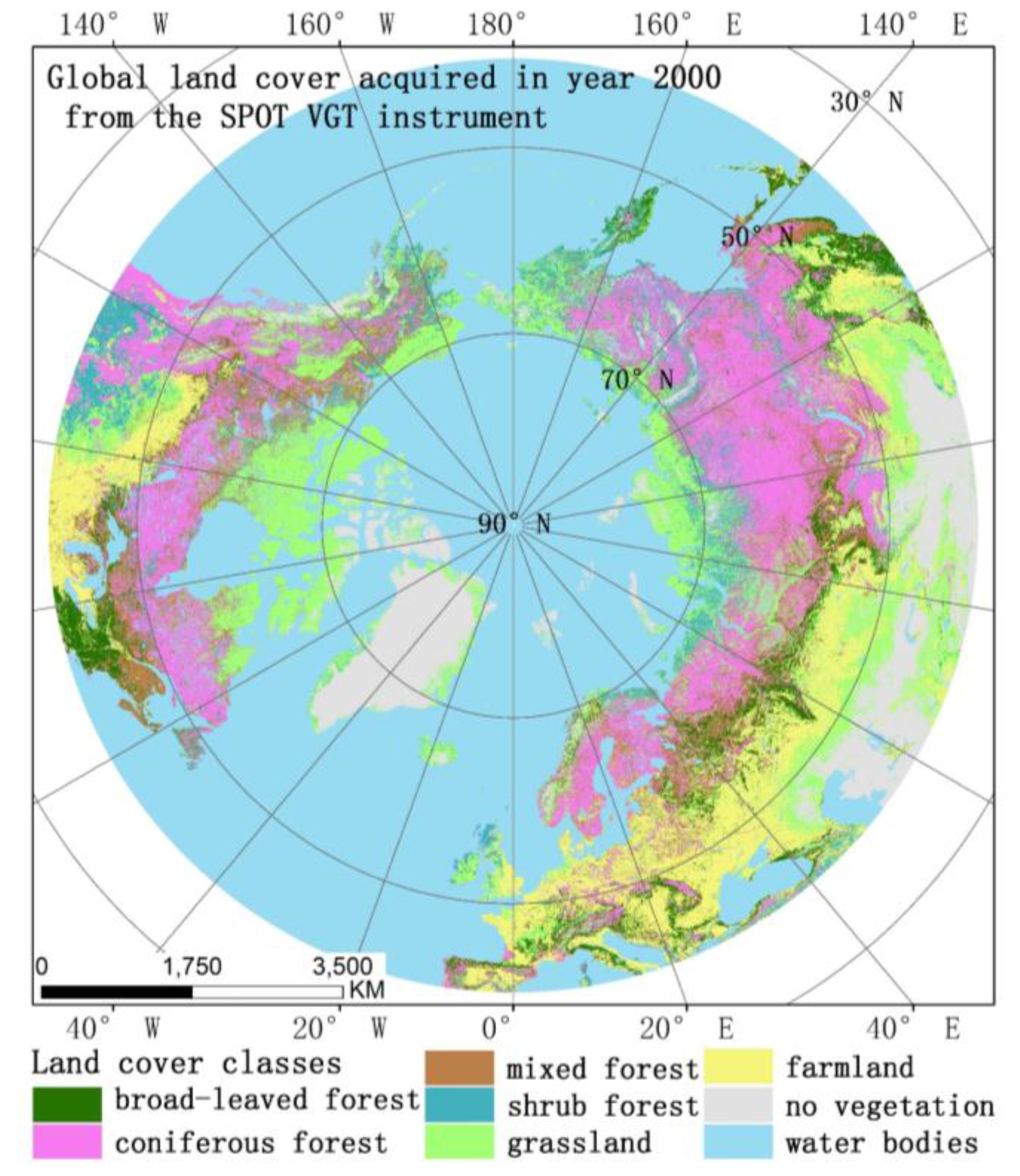
2.2. Land Cover Data

A land cover map was used for analysis of and discussion on the agreement and discrepancies of vegetation phenology for different land cover types. We chose the Global Land Cover 2000 (GLC-2000) [32] dataset for this study. The GLC-2000  [32] land cover product was used because it was based primarily on SPOT vegetation daily 1 km data and because of the independence of the GIMMS dataset [10]. The GLC 2000 land cover classes were reclassified into 8 major land cover classes: Broad-leaved forest; coniferous forest; mixed forest (coniferous + broad-leaved); shrub forest; grassland; farmland; no vegetation; and water bodies (Figure 1).

2.3. Climate Data

To further analyze whether the temperature change had an impact on vegetation phenology changes, the Northern Hemisphere land temperature anomalies data from 1880 to 2014 were download from NOAA's National Centers [33]. The term temperature anomaly means a departure from a reference value or long-term average. A positive anomaly indicates that the observed temperature was warmer than the reference value, while a negative anomaly indicates that the observed temperature was cooler than the reference value [34]. In this paper, we used temperature anomalies from 1982 to 2013 for our analysis.

2.4. Phenology Metrics

Currently, products of long time-series datasets commonly use the Maximum Value Composite (MVC) method, including GIMMS 15-day MVC products, MODIS 8-day products, 16-day MVC products, and SPOT VGT 10-day MVC products. However, due to the effects of cloud, atmosphere, sensor, and surface bidirectional reflectance, the original NDVI time-series, which has been synthesized, partially contains singular values. Performance limitations utilizing these data are perceptible, especially in a single cell where the main focus is the phenomenon of a NDVI time-series dip in the graph or a needlepoint hump. Singular values affect dataset precision, necessitating a further process to reduce the influence of the noise and provide more effective time-series datasets.
Figure 1. Main vegetation types of the study area [32].
Remotesensing 07 10973 g001
Many scholars have proposed several reconstruction algorithms for time-series, such as the best index of slope extraction method [35], the average iterative filtering method [36], the Fourier transform method [37], the Savitzky-Golay filtering method [13,38,39,40], the Asymmetric Gaussian fitting method [39,41], the wavelet analysis method [42], and linear interpolation within the time window [43]. The accuracy of remotely-sensed data in a time-series requires a noise smoothing process to remove leakage points or vacancy points within the series. TIMESAT software [41,44] is among the most widely used programs [10,11,45,46,47,48]. To reduce drop-outs or gaps from long time-series data, TIMESAT uses Savitzky-Golay filtering, asymmetrical Gaussian or double logistic functions to fit NDVI data [10,11,45,46,47,48]. The Savitzky-Golay filter smooths out noise in NDVI time-series, specifically noise caused primarily by cloud contamination and atmospheric variability. It is more effective in obtaining high-quality NDVI time-series. Many studies that use the Savitzky-Golay smoothing model for data filtering obtain good results. The Savitzky-Golay (S-G) filtering method was applied in this study to fit the time-series data (Equation (1)).
The calculating formula for the S-G is as follows:
Y j * = i = m i = m C i Y j + 1 2 m + 1
where Yj* is the reconstructed data, Ci is the least squares filter coefficient, j represents the original coordinates of the sliding window, Yj+1 represents the j-th original values of the sliding window, and 2m + 1 is the width of the sliding window.
We employed TIMESAT to generate smooth time-series NDVI data. We adopted the adaptation strength of 2.0, no spike filtering, seasonal parameter of 0.5, Savitzky-Golay window size of 2, and amplitude season start and end of 30% to calculate the phenology parameters. We calculated the SOS and EOS for each year and obtained LOS as the difference between SOS and EOS in each grid point [49].

2.5. Statistical Analysis

The variation of vegetation phenology were analyzed at pixel and regional scale, spatial and temporal scales in this paper.
The average values of SOS, EOS, and LOS were calculated over the past 32 years (1982–2013) to evaluate the spatial patterns phenology metrics. Spatial trends of phenology were examined by applying a simple linear regression model with time as the independent variable and phenology metrics as the dependent variable. The outputs of the trend analyses are maps of regression slope values at the 95% confidence level, indicating the magnitude of the calculated trend. The spatial distribution of long-time series phenological variation for each pixel can be obtained. It can provide finer-scale analysis of the variation of phenological characteristics for the different region or land cover types in pixel and spatial scale.
To research the trend of phenology at the hemispheric scale, we calculated the average of the phenological parameters for the entire study area above 40°N in the Northern Hemisphere using the ordinary least squares (OLS) approach. To evaluate the trend of phenology in different land cover types and different time periods, the regional average trends were calculated for the different land cover types using OLS. The r and p values of the linear trend were calculated using OLS for the average of the different vegetation types in 1982–2001, 2002–2013, and 1982–2013. The average phenology values for entire study area or different land cover types were calculated using the zonal statistic tool in ArcGIS. This method ignores individual or local differences, while it can reflect the whole variation of phenological characteristics in the entire study area or different vegetation types in regional and temporal scale.
To understand how changes in phenology are associated with climate change, a correlation analysis was applied to examine the relationship between phenology metrics and temperature anomalies (1982–2013) in the Northern Hemisphere. Pearson’s correlation coefficients (r) were calculated between phenology metrics (SOS, EOS, and LOS) and temperature anomalies from January to December for different land cover types.

3. Results and Discussion

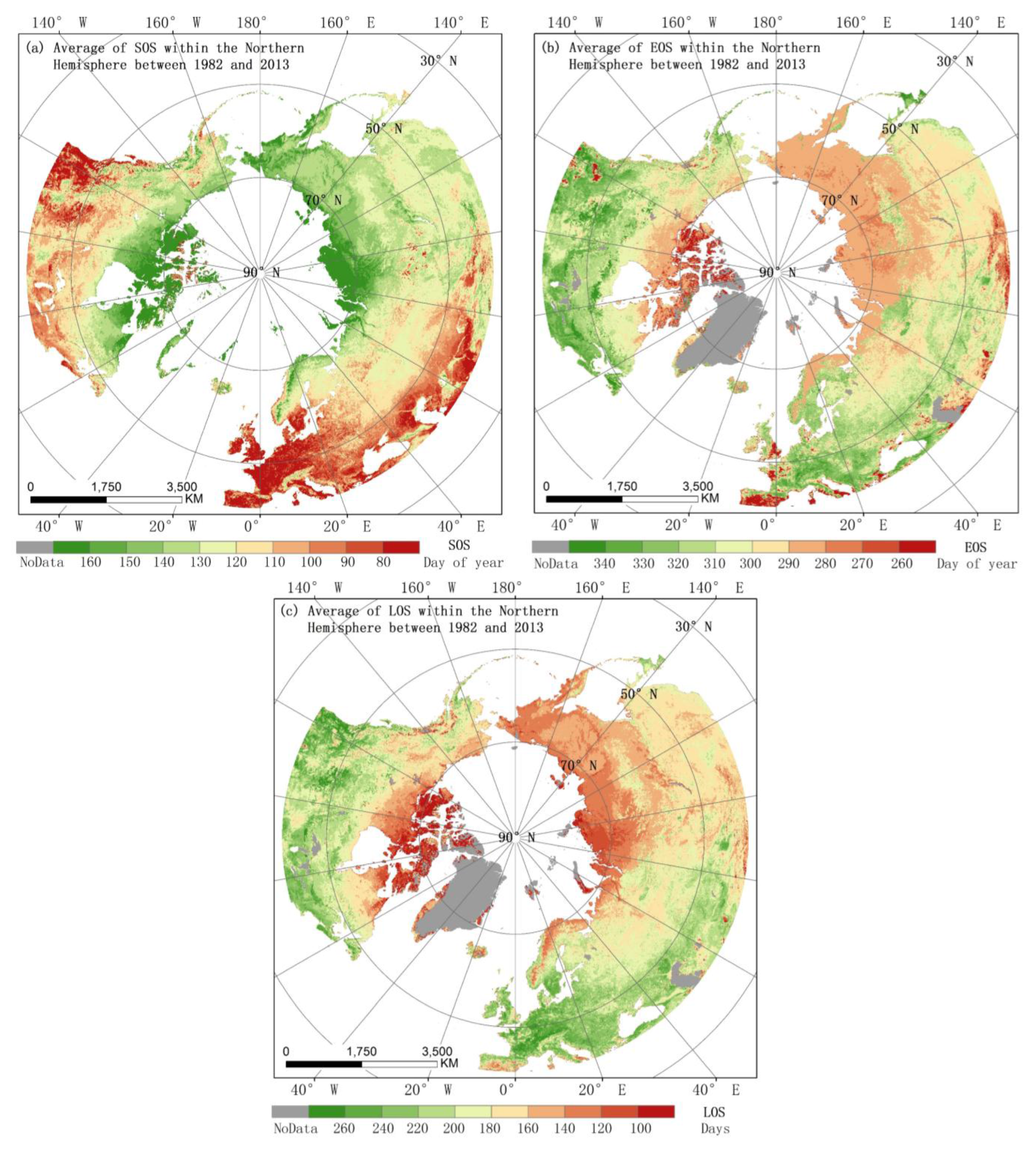
3.1. Spatial Patterns of Vegetation Phenology

The mean phenological parameter data were calculated on a pixel scale at the middle and high latitudes of the Northern Hemisphere over nearly 32 years (1982–2013). Clearly, the spatial distribution of phenology shows obvious variability in the study area (Figure 2).
Figure 2. Averages of start of season (SOS, a), end of season (EOS, b), and length of season (LOS, c) within the Northern Hemisphere between 1982 and 2013.
Remotesensing 07 10973 g002
The SOS of vegetation was mainly distributed in the range of 80–160 days (Figure 2a). In addition, the SOS presented significant differences with latitude change and was gradually delayed with increasing latitude. A SOS earlier than 80 days mainly occurred at 40°N–60°N in North America and Southern Europe. The latest SOS (greater than 160 days) occurred above 70°N within the Arctic Circle. At the same latitudes, later SOS dates occurred in Asia than in Europe and North America.
Compared with the SOS, the EOS exhibited an opposite trend in spatial distribution (Figure 2b); thus, the EOS advanced with increasing latitude. The earliest EOS occurred within the Arctic Circle (earlier than 260 days), whereas the latest EOS occurred at low latitudes in North America and Europe (later than 330 days). The EOS was distributed in the range of 280–300 days over the vast majority of Asia.
The LOS mostly varied from 100 to 260 days and gradually extended from high to low latitudes over the entire study area (Figure 2c). The shortest LOS was found in the Arctic Circle, where it lasted less than 100 days in most areas. The study area was divided into three large zones by different colors according to the LOS (Figure 2a): A LOS of less than 150 days, which was mainly above 60°N in Asia and North America and above 70°N in Europe; a LOS of 150–200 days, which mainly occurred at 40°N–60°N in Asia and 50°N–60°N in North America; and a LOS of greater than 200 days, which mainly occurred below 50°N in Europe and North America.

3.2. Trends in Phenology

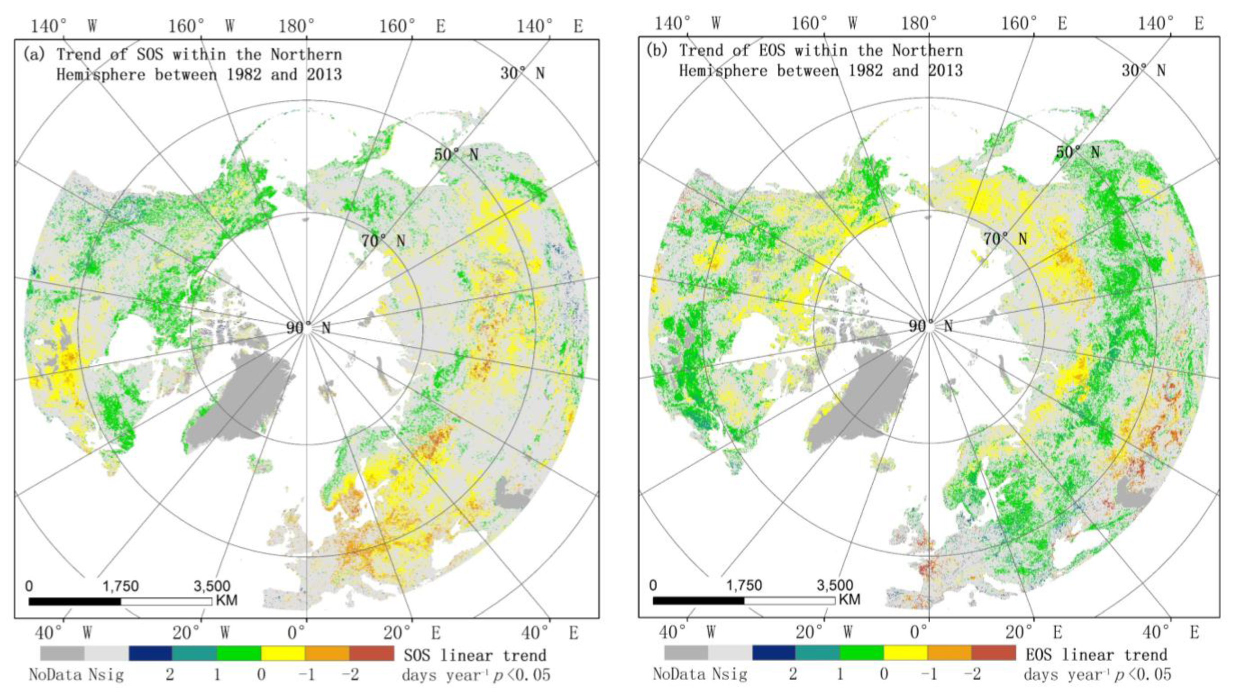
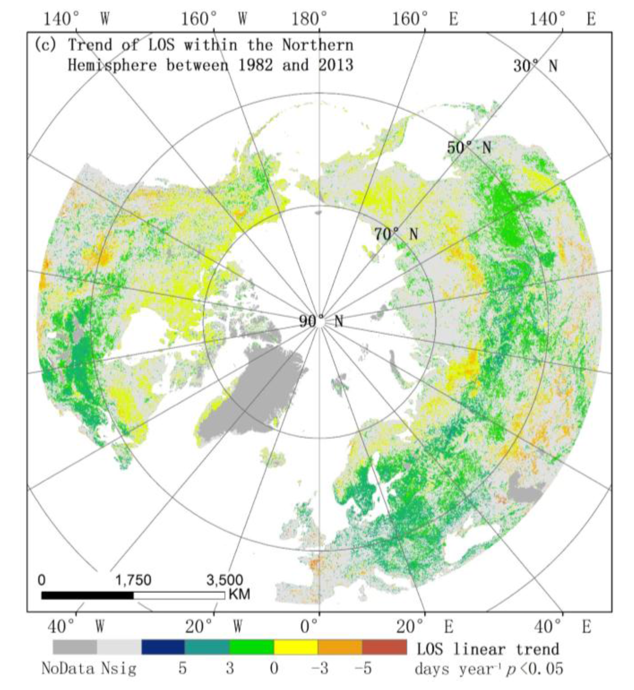
3.2.1. Spatial Patterns of Phenological Trends

The linear trends of the SOS, EOS, and LOS were calculated at the 95% confidence level (Figure 3). Over the past 32 years (1982–2013), the SOS trend was significant, accounting for 24.63% of the pixels and exhibiting either advanced or delayed trends (p < 0.05). Pixels with a negative (advanced) trend of the SOS accounted for 56.5% of the total pixels and exhibited a significant trend (p < 0.05), which was slightly greater than pixels with a delayed trend (p < 0.05). Negative SOS trends mainly occurred in the eastern United States, Europe, and Russia (Asia), whereas pixels with positive (delayed) trends mainly occurred above 50° N in North America.
Figure 3. Trends of the start of season (SOS, a), end of season (EOS, b), and length of season (LOS, c) within the Northern Hemisphere between 1982 and 2013 (A positive trend indicates that the delayed trend for SOS, delayed trend for EOS and extended for LOS, while a negative trend indicates that the advanced trend for SOS, advanced trend for EOS and shortened trend for LOS).
Remotesensing 07 10973 g003aRemotesensing 07 10973 g003b
For the EOS, 31.7% of pixels over the entire study area showed significant changes, and pixels with a delayed trend accounted for 58.7% of the total. Delayed EOS mainly occurred at 40°N–60°N, especially in the United States (North America), Europe, and Mongolia (China in Asia). In addition, the EOS exhibited an advanced trend above 60°N in Eurasia.
The spatial trends of the LOS were a combination of the trends for the SOS and EOS (Figure 3c). Over the entire study area, 34.9% of the pixels displayed significant changes. Shortening of the LOS (p < 0.05) mainly occurred in Canada (North America) and Russia (Asia), whereas extension occurred mainly at 50°N–60°N (p < 0.05).

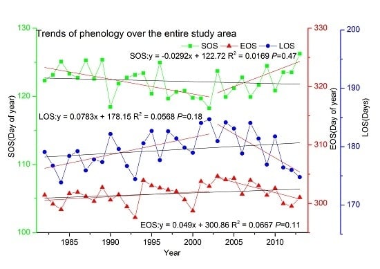
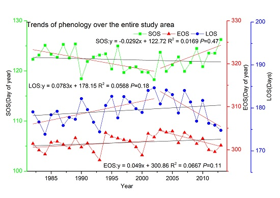
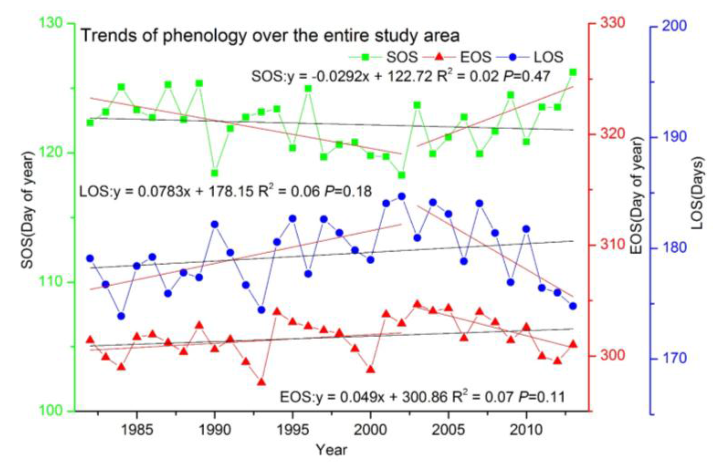
3.2.2. Trends over the Entire Study Area

The average trends of the phenological parameters were calculated for the entire study area in the high latitudes of the Northern Hemisphere. The entire study area included all vegetation types.
The SOS, EOS, and LOS displayed two distinct change trends, with 2002 serving as the cut-off point (Figure 4). The SOS advanced, the EOS delayed, and the LOS extended significantly from 1982 to 2002, although the opposite trends occurred for 2003–2013. In the initial two decades, the SOS advanced by −2.2 ± 0.6 days·decade−1 (p < 0.05). When the time scale was extended to 2013, the trend of advanced SOS dropped to −0.29 ± 0.4 days·decade−1 (p = 0.47), which was primarily because of the trend of delayed SOS after 2003 (3.2 ± 1.7 days·decade−1, p = 0.09). The EOS was delayed over the past 32 years by 0.49 ± 0.3 days·decade−1 (p = 0.11), and the degree of the EOS changes was similar to that of the SOS changes, with a turning point at 2002. In the initial period (1982–2002), the EOS was moderately but not significantly delayed by 0.78 ± 0.6 days·decade−1 (p = 0.15); in the latter period (2003–2013), the EOS was delayed by 4.5 ± 0.9 days·decade−1 (p < 0.05). Compared with the SOS, the LOS was extended by 0.78 days·decade−1 (p = 0.18) over the past 32 years, and it was extended by 2.9 days·decade−1 (p < 0.05) from 1982 to 2002, with an opposite trend of 7.7 ± 2.2 days·decade−1 (p < 0.05) from 2003 to 2013. Clearly, the increasing trend of the LOS in the prior two decades was smaller than the decreasing trend of the LOS in the most recent decade. These results indicate that the trends of advanced SOS, delayed EOS, and increased LOS were slow over the past 32 years. Although significant changes occurred in vegetation phenology over the initial 21 years, the trends were obviously reduced over the latter 11 years and tended to recover to the level of phenological changes in the 1980s at the middle and high latitudes of the Northern Hemisphere.
Figure 4. Trends of start of season (SOS), end of season (EOS), and length of season (LOS) over the Entire Study Area (Green square, red triangle and blue dot represent the average of SOS, EOS and LOS, respectively. Yearly mean phenology values were calculated used all pixels for entire study area).
Remotesensing 07 10973 g004

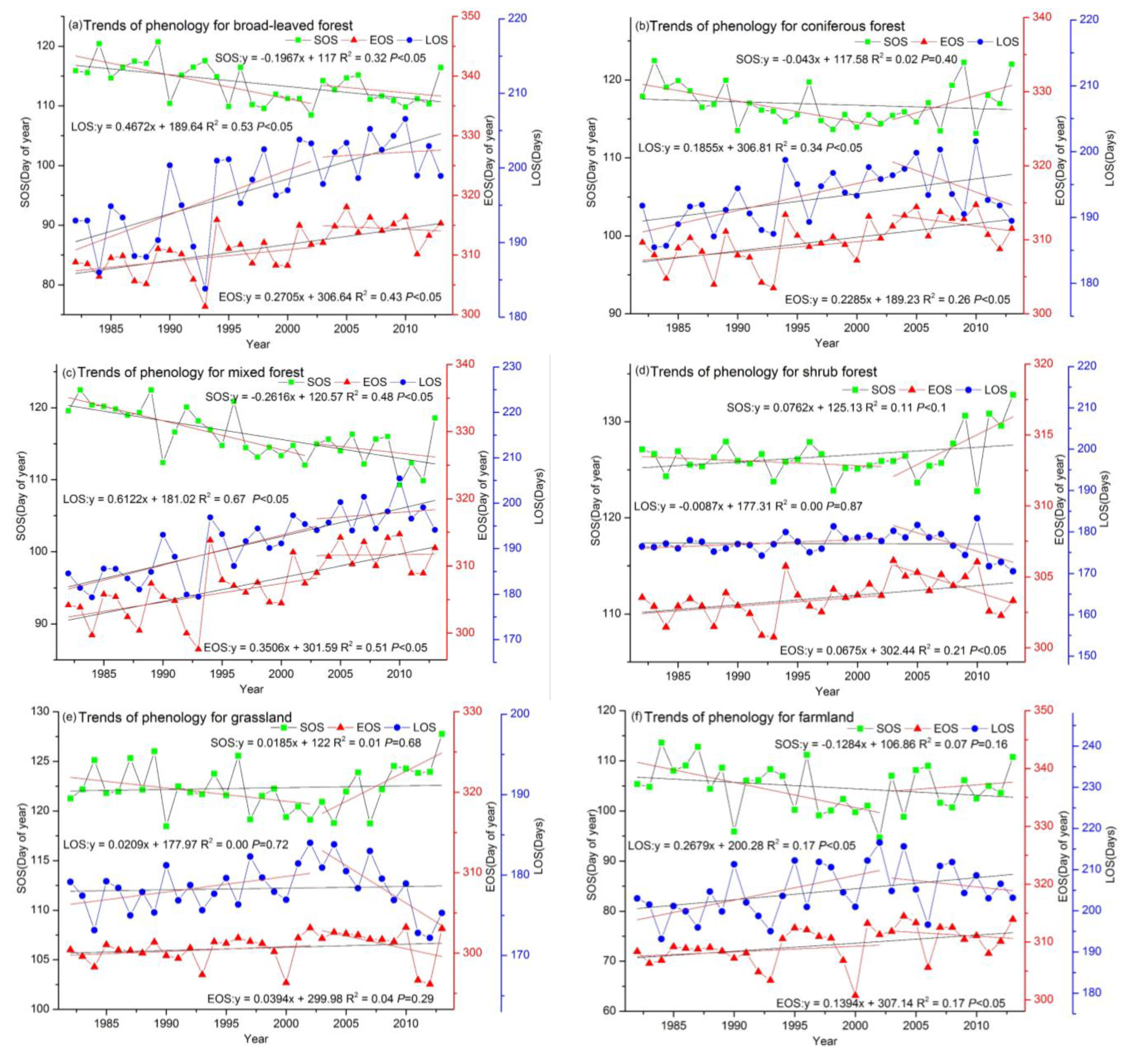
3.2.3. Phenological Trends for Different Land Cover Types

To analyze the phenological trends of different land cover types, this study selected six vegetation types in the study area as its major subjects: Broad-leaved forest (a), coniferous forest (b), mixed forest (c), shrub forest (d), grassland (e), and farmland (f) (Figure 5 and Table 2). The r and p values of the linear trend in Table 2 were calculated using OLS for 1982–2001, 2002–2013, and 1982–2013.
The linear trends of vegetation phenology for the period 1982–2013 were calculated with respect to the SOS, EOS, and LOS for the different vegetation types over the entire the study area (Figure 5). The trends of the SOS, EOS, and LOS showed substantially different characteristics according to vegetation type (Figure 5a–f). For broad-leaved forest and mixed forest, the SOS significantly advanced over the entire study area over the past 32 years at the 95% confidence level (Figure 5). Among the different vegetation types, the trend of advanced SOS was most significant for mixed forest (−2.6 ± 0.5 days·decade−1, p < 0.05), followed by broad-leaved forest (2 ± 0.5 days·decade−1, p < 0.05). No significant trend in the SOS was observed for the other vegetation types at the 95% confidence level. Among the six vegetation types from 1982 to 2013, the LOS trends were most significant for mixed forest (6.1 ± 0.8 days·decade−1, p < 0.01), followed by broad-leaved forest (4.7 ± 0.8 days·decade−1, p < 0.01), and the LOS of coniferous forest advanced by 2.3 ± 0.7 days·decade−1 (p < 0.01).
Figure 5. Trends of start of season (SOS, a-f), end of season (EOS, a-f), and length of season (LOS, a-f) for different land cover types (Green square, red triangle and blue dot represent the average of SOS, EOS and LOS, respectively. Yearly mean phenology values were calculated used all pixels for different land cover types).
Remotesensing 07 10973 g005
All vegetation types showed delayed EOS over the period from 1982 to 2013 (Figure 5). The greatest trend occurred in mixed forest (3.5 ± 0.6 days·decade−1, p < 0.05), followed by broad-leaved forest (2.7 ± 0.6 days·decade−1, p < 0.05), coniferous forest (1.9 ± 0.5 days·decade−1, p < 0.05), farmland (1.3 ± 0.6 days·decade−1, p < 0.05), and shrub forest (0.7 ± 0.2 days·decade−1, p < 0.05). The trend of delayed EOS was not significant for grassland.
The different vegetation types showed extended LOS to varying degrees over the past 32 years (Figure 5). The trend of extended LOS was significant for broad-leaved, coniferous, and mixed forests and for farmland but not for shrub forest or grassland. For broad-leaved forest, coniferous forest, mixed forest, and farmland, the LOS was extended by 4.7 ± 0.8 days·decade−1, 2.3 ± 0.7 days·decade−1, 6.1 ± 0.8 days·decade−1, and 2.7 ± 1 days·decade−1, respectively (all p < 0.05). Apparently, the trend of the LOS was jointly affected by those of the SOS and EOS, although delayed EOS had a greater effect. Thus, the trend of delayed EOS was greater than that of advanced SOS for vegetation in the Northern Hemisphere. The phenological trends were significant for woody plants, especially for broad-leaved deciduous trees, but not for herbaceous plants.
Table 2. The trends of phenology for different vegetation types in three time periods (a-broad-leaved forest, b-coniferous forest, c-mixed forest, d-shrub forest, e-grassland, and f-farmland. A positive trend value indicates that the delayed trend for SOS, delayed trend for EOS and extended for LOS, while a negative trend value indicates that the advanced trend for SOS, advanced trend for EOS and shortened trend for LOS).
1982–20022003–20131982–2013
SOSa−0.37 0.018−0.20
b−0.28 0.44 *−0.04
c−0.38 −0.06−0.26
d−0.060.54 0.08 *
e−0.110.61 0.02
f−0.42 0.52−0.13
EOSa0.190.030.27
b0.14−0.080.19
c0.27 *0.180.35
d0.06−0.19 *0.068
e0.02−0.320.040
f0.07−0.100.14
LOSa0.56 0.020.47
b0.41 −0.530.23
c0.65 0.240.61
d0.12 *−0.71 −0.01
e0.13−0.93 0.02
f0.49 −0.630.26
* p < 0.1, p < 0.05, p < 0.01
The entire study area (Figure 4), coniferous forest (Figure 5b), shrub forest (Figure 5d), and grassland (Figure 5e) have the same change trends for the two time periods (1982–2002 and 2003–2013). The proportion of these three vegetation types was 62.6%, and the change trend of phenology in the entire study area was close to that in the three vegetation types. The LOS of broad-leaved forest (Figure 5a) and mixed forest (Figure 5c) over the past 32 years showed a strong increased trend, and simultaneously, the SOS and EOS showed an advanced trend and a delayed trend, respectively. The increased rate of LOS for coniferous forest (Figure 5b), shrub forest (Figure 5d), and grassland had an obvious decelerating trend over the last decade.

4. Discussion

4.1. Trends in Phenology

In this study, the majority of advanced SOS trends occur in Europe and Asia, with a minority occurring in North America. These results are supported by the conclusions of Barichivich [4], Wang [27], and Cohen [50]. Regions with significantly delayed EOS are mainly distributed in North America, followed by Europe. This result is consistent with the conclusion of Zhu et al. [25], who showed that the LOS was extended mainly because of the delayed EOS in North America. Jonathan et al. [4] reported that the LOS was significantly extended in Eurasia, although significant changes were not observed in North America. From the spatial distribution of change trends on the pixel scale (Figure 3), the trend of the SOS is negative (advanced) for 56.5% of the pixels over the entire study area at the 95% confidence level. The trend of advanced SOS is most significant in Europe, followed by North America. In certain regions, the advanced SOS and delayed EOS trends occur simultaneously, thus enhancing the extended LOS trend. In addition, the SOS and EOS trends counteract each other in certain regions, thus diminishing the trend of extended LOS. Because the large-scale study area has different vegetation types, climatic zones, and water/heat conditions, the positive and negative change trends of pixels offset the average change trends. Over the long time-series, the phenological trends are not significant over the entire study area from 1982 to 2013. However, different trends are observed, and 2002 is the cut-off point. Significant changes occur in the initial 21 years (1982–2002), with the SOS advancing by 2.2 ± 0.6 days·decade−1 (p < 0.05). This result strongly supports previous findings on the advancing trend of the SOS in the middle and high latitudes of the Northern Hemisphere prior to 2000 [20,26,27]. In the latter 11 years (2003–2013), the phenological trends are the opposite, with the SOS delayed by 3.1 ± 1.7 days·decade−1 (p < 0.1), the EOS advanced by 4.5 ± 0.9 days·decade−1 (p < 0.05), and the LOS shortened by 7.7 ± 2.2 days·decade−1 (p < 0.05). As reported by Zeng and Jeong et al. [6,26], the phenological trends from 2000 to 2008 are obviously lower than the change rates from 1982 to 1999 and do not display strong significance. The SOS advances by −1.6 ± 0.8 days·decade−1 (p < 0.1) over the entire study area from 1982 to 1999, which is slightly slower than the value of 3.1 days·decade−1 over the entire Northern Hemisphere reported by Jeong et al. [26]. The advance of the SOS is reduced in the Northern Hemisphere over the past 31 years compared with that over the initial 21 years, and an opposite SOS trend occurs in the most recent 11 years. This observation is similar to the results of Wang et al. [27], who indicate that SOS trends are reduced at 30°N–72°N in the Northern Hemisphere over the past three decades compared with the initial two decades.

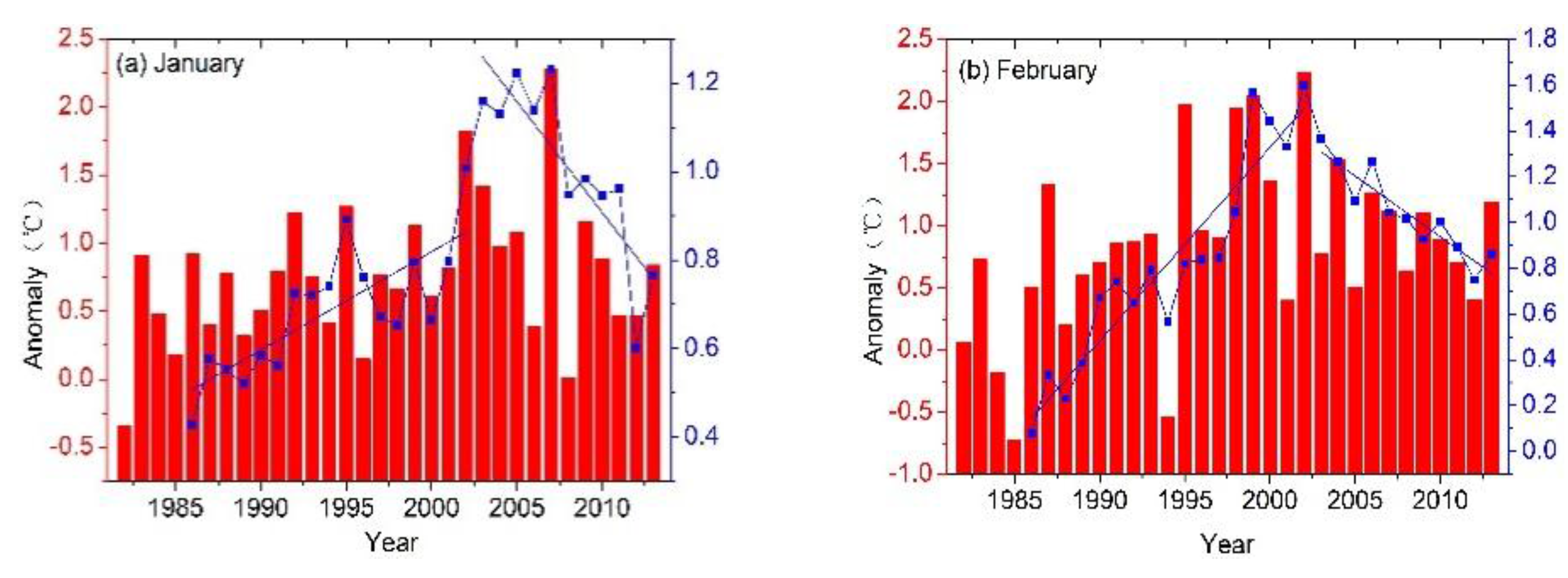
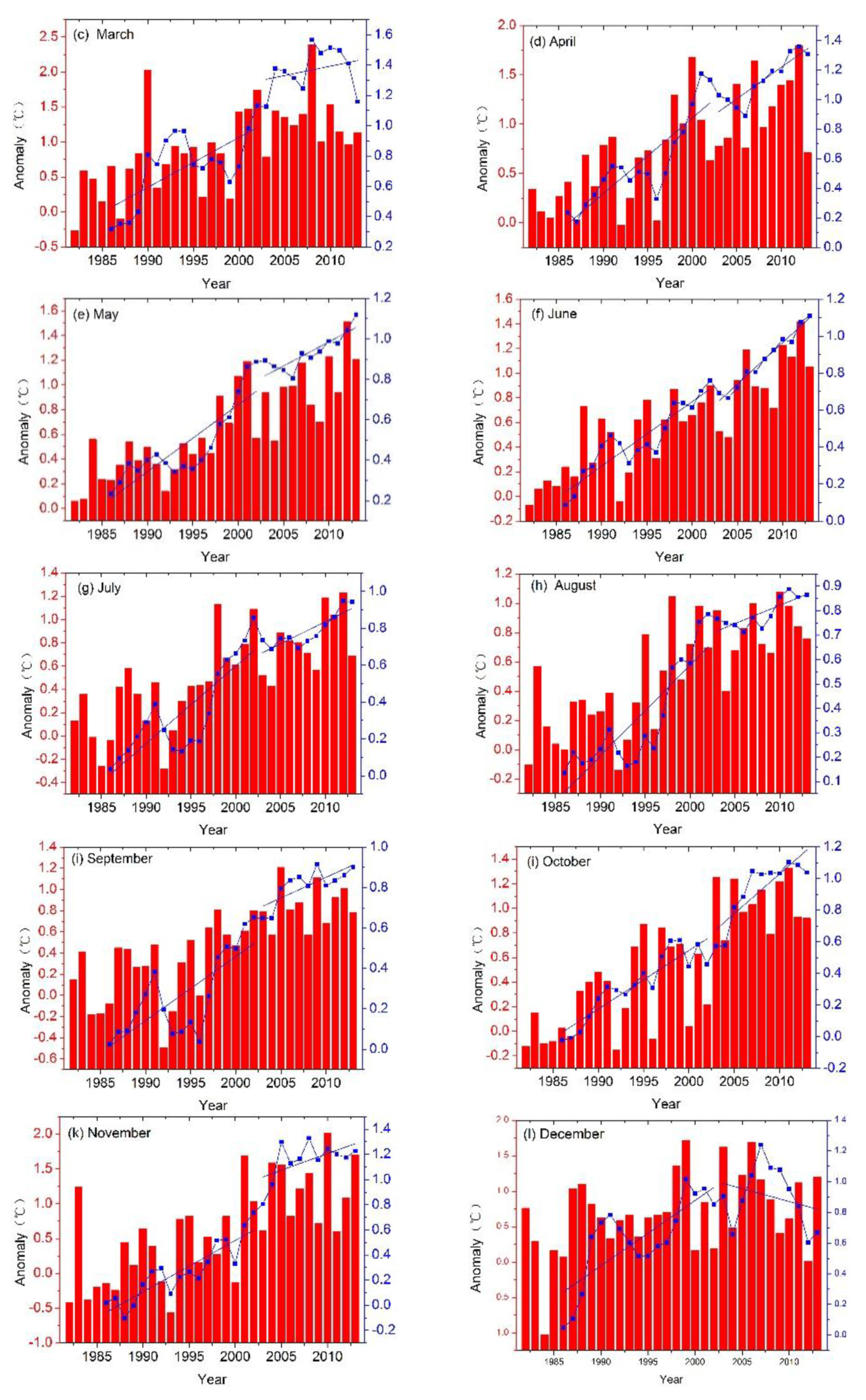
4.2. Climate Change and Phenology

This study shows that the delay trend of SOS and the advance trend of EOS decelerate and even reverse after 2002. Wang et al. [27] also showed that the advanced SOS in the Northern Hemisphere has decelerated or reversed over the last decade. The results of Jeong et al. [26] showed that the SOS advanced 5.2 days from 1982 to 1999 but only advanced 0.2 days from 2000 to 2008 and that the EOS had the same decelerating trend in the subsequent time period. These conclusions [26,27] also support our results that the advanced trend of SOS, the delayed trend of EOS, and the extended trend of LOS have decelerated over the last decade. Some authors show a shortened LOS for crops [51,52,53,54], whereas others authors’ results show an extended LOS [55,56]. Indeed, we have also observed a different SOS, EOS, and LOS across the different locations (Figure 3a–c). There have been large differences for the EOS and LOS in different continents and latitudes. Although we divide the study area into six vegetation types to analyze the phenology trends in different vegetation types, there has been a problem of mixed species in the large scale of the study area. Figure 3 shows that most pixels did not have significant trends for the entire study areas, with only 24.63% pixels of the SOS having a significant trend. These results offset some of the positive and negative trends when the large regional trends are calculated.
The large interannual variations in winter and spring climate significantly affect the interannual variations in the SOS [57]. Global warming deceleration over the past decade has been observed, and a variety of mechanisms have been suggested to explain it [58,59,60,61,62,63]. The Northern Hemisphere land temperature anomalies data from 1982 to 2013 were calculated (Figure 6), and the correlation between the temperature anomalies and phenology parameters was obtained (Table 3). The hottest 30 years recorded since 1880 have all occurred in the past three decades. However, the rate of increase since 2000 is higher than the rate of increase before 2000. The temperatures have slowed the trend after 2000, and temperature anomalies have decreased since 2003 in January and February. Since 2003, temperature anomalies show a downward trend from January to March and July to December, but the same trend from April to June does not appear. These temperature trends have a great influence on vegetation phenology changes. There were no significant correlation coefficients for shrub forest and grassland with temperature anomaly, but there were strong correlations for broad-leaved forest, coniferous forest, and mixed forest phenology parameters (Table 3). Although temperature is considered to be the main factor that affects grass phenology, water availability has also been identified as a key factor for grass phenology [64] Our results showed no significant correlation coefficient between grassland and temperature (Table 3). Previous studies suggest that climate change plays a dominant role in crop phenology [65,66,67]; in this paper, the results showed that there is a good correlation for the SOS from January to April, for the EOS from September to November, and for the LOS from January to November. Although the total length of the time periods is 32 years, it is short compared to the entire climate change time period. The phenology changes mainly caused by climate change also need to be examined. Although we strive to reduce the impact of noise, some interference remains, including fires, land use changes, etc.
Figure 6. (a–l)The monthly temperature anomaly form 1982 to 2013 (Monthly temperature anomaly means a departure value from long-term average from 1880 to 2014 for every month).
Remotesensing 07 10973 g006aRemotesensing 07 10973 g006b
Table 3. The relationship between phenology of different vegetation types and monthly temperature anomaly (a-broad-leaved forest, b-coniferous forest, c-mixed forest, d-shrub forest, e-grassland and f-farmland. Monthly temperature anomaly means a departure value from long-term average from 1880 to 2014 for every month).
JanFebMarAprMayJunJulAugSepOctNovDec
aSOS−0.35−0.45 −0.54 −0.70 −0.46 −0.62 −0.60 −0.65 −0.58 −0.51 −0.51 −0.14
EOS0.20.030.49 0.55 0.61 0.62 0.54 0.58 0.64 0.67 0.77 0.2
LOS0.32 *0.270.61 0.73 0.64 0.73 0.67 0.73 0.73 0.70 0.77 0.21
bSOS−0.34 *−0.28−0.31 *−0.43 −0.27−0.30 *−0.29−0.28−0.17−0.23−0.11−0.21
EOS0.190.0950.41 0.49 0.47 0.49 0.50 0.57 0.62 0.68 0.70 0.31 *
LOS0.35 *0.240.48 0.62 0.51 0.53 0.54 0.58 0.55 0.63 0.57 0.36
cSOS−0.36 −0.37 −0.59 −0.84 −0.70 −0.79 −0.72 −0.72 −0.66 −0.66 −0.51 −0.19
EOS0.220.060.48 0.59 0.62 0.65 0.57 0.64 0.69v0.73 0.77 0.27
LOS0.32 *0.220.61 0.81 0.76 0.82 0.74 0.78 0.79 0.81 0.76 0.27
dSOS−0.15−0.0900.030.110.160.0440.020.190.150.1340
EOS0.240.110.35 0.45 0.42 0.37 0.42 0.54 0.56 0.58 0.58 0.32 *
LOS0.250.130.180.210.120.060.180.260.130.180.190.15
eSOS−0.38 −0.19−0.35 −0.250.10.050.04−0.07−0.040−0.050
EOS0.270.190.19−0.120.030.10.120.160.20.250.49 0.35
LOS0.47 0.270.40 0.11−0.060.030.0450.160.150.170.36 0.23
fSOS−0.33 −0.43 −0.60 −0.49 −0.17−0.36 −0.36 −0.38 −0.32 *−0.27−0.39 −0.06
EOS0.230.050.230.20.32 0.36 0.36 0.37 0.46 0.50 0.63 0.2
LOS0.37 0.36 0.59 0.49 0.30 0.47 0.48 0.50 0.49 0.47 0.64 0.15
* p < 0.1, p < 0.05, p < 0.01

4.3. The Influence of Other Factors on Vegetation Phenology

The time period (1982–2013) investigated in the present study is relatively long and exhibits changes in the vegetation types of the Northern Hemisphere. In this study, only temporal-spatial variation in phenology is analyzed to understand the characteristics of vegetative growing seasons. However, many factors (such as temperature, precipitation, soil moisture, land cover changes, and disturbances) may contribute to changes in vegetation phenology. For example, cultivated land is most significantly affected by human factors, resulting in uncertain long-term variation trends in the vegetation phenology. The variation in phenology may be the result of changes in soil moisture due to an increase in precipitation rather than an increase in temperature. However, relatively good natural conditions have been maintained in certain areas over the past 32 years, reflecting the growth processes of natural vegetation. When studying long-term vegetation phenological and climatic changes, areas where good natural conditions have been maintained may better reflect the impact of climate change.
In this study, the phenology parameters are determined only by remote sensing data. The effects of the Bidirectional Reflectance Distribution Function (BRDF) on the NDVI remain as noise. Given that the BRDF is wavelength-specific, different reflectances are affected differently throughout the year, not only because of the change in the biophysical properties of the target but also because of the variable viewing and illumination geometry. Although the MVC method and time-series analysis can be considered to reduce the remaining noise, some BRDF bias may continue to remain in the GIMMS 3g NDVI data. Bhandari et al. [68]  reported that BRDF correction can have a significant impact on the phenological parameters. The BRDF effects are different from one environment to another, and more studies in different environments may be useful to obtain better insight [68]. The NDVI derived from the BRDF/albedo parameters product has clear benefits for monitoring vegetation phenology.
The phenologies for different types of crops are different; however, due to the low resolution of the data source, 8-km spatial resolution data have mixed pixels for crops. The land cover product is used in this study only to obtain the primary classification of farmland. There are no more finely grained categories for the types of crops planted. The phenology parameters are calculated based on the average value for all crops. The time period for the different types of crops planted cannot be distinguished. In future works, we can use higher resolution remote sensing data to analyze some vegetation or crop types
Despite the advantages of remote sensing over field observations, remote sensing data include a number of uncertainties. For example, remote sensing data are affected by the sensor and atmosphere, which can result in substantial noise. In addition, vegetation is often affected by external factors, such as winds, pests, fires, and human activities, which all have strong impacts on vegetation. Although this study performed noise reduction by filtering, the impact of external factors cannot be completely removed, and the presence of certain types of interference results in uncertainties in the extracted results for the phenological parameters.

5. Conclusions

This study uses vegetation phenology at the middle and high latitudes of the Northern Hemisphere as the study subject. An inversion of phenological parameters is performed using the GIMMS NDVI3g datasets for the period 1982–2013 to analyze the spatial patterns of means, spatial patterns of trends, spatial trends over the entire region, and different vegetation types. The main findings can be summarized as follows:
With respect to the spatial distribution of multi-year mean data, the SOS was generally delayed from low to high latitudes, and the EOS was progressively advanced in the Northern Hemisphere. Regarding the spatial distribution of phenological trends, the SOS showed a trend of significant advancement in Europe over the past 32 years, followed by North America, and the trend of advanced SOS was significant at high latitudes in Asia.
The phenology change trends did not increase with increasing latitude, and obvious changes primarily occurred at 50°N–70°N. These trends consist of advanced SOS, delayed EOS, and increased LOS. These areas consist mainly of forest. The trend of phenology is not obvious in grassland areas. This phenomenon may be largely related to the vegetation types.
On the study-area scale, SOS trends were significant at the middle and high latitudes (≥40°N) of the Northern Hemisphere over the past 32 years. Collectively, our results indicate that the trends of advanced SOS at the middle and high latitudes of the Northern Hemisphere from 1982 to 2013 were reduced or even reversed in the most recent decade.
The phenological trends are different with different vegetation types. The SOS trends of woody vegetation were significant and obviously higher than those of herbaceous vegetation at the middle and high latitudes of the Northern Hemisphere. Significant changes in the SOS were not observed for herbaceous vegetation. The trend of delayed EOS was greater than the trend of advanced SOS at different scales. Clearly, the EOS of vegetation has a strong response to climate change. Coniferous forest, shrub forest, grassland, and the entire study area have the same change trends for the two time periods (1982–2002 and 2003–2013), and the increased rate of the phenology parameters has decelerated over the last decade. The LOS of broad-leaved forest and mixed forest in the past 32 years shown a strong increased trend, and simultaneously, the SOS and the EOS shown an advanced trend and a delayed trend, respectively.
The results of this study strongly support the research on advanced SOS, delayed EOS, and increased LOS at the middle and high latitudes of the Northern Hemisphere over the initial two decades. Simultaneously, the change rate has decelerated over the most recent decades.

Acknowledgments

The authors would like to thank the entire GIMMS group for permitting the usage of the NDVI3g dataset. We thank Per Jonsson and Lars Eklundh for making available their TIMESAT routine. This study was supported by China Postdoctoral Science Foundation (Grant No. 2014M561272), the Science and Technology Development Project of Jilin Province (Grant No. 20150520069JH), Jilin Postdoctoral Science Foundation (Grant No. RB201353), the Fundamental Research Funds for the Central Universities (Grant No. 14QIVJJ025 and 11SSXT134) and National Natural Science Foundation of China (Grant No. 41501449 and 41371394).

Author Contributions

All authors contributed significantly to this manuscript. Specific contributions include data collection (Jianjun Zhao, Xiaoyi Guo), data analyses (Jianjun Zhao, Xiaoyi Guo, Chun Chen), methodology (Jianjun Zhao, Hongyan Zhang, Zhengxiang Zhang), and manuscript preparation (Jianjun Zhao, Hongyan Zhang, Zhengxiang Zhang, Xuedong Li).

Conflicts of Interest

The authors declare no conflict of interest.

References

  1. Parry, M.L.; Canziani, O.F.; Palutikof, J.P.; van der Linden, P.J.; Hanson, C.E. IPCC, 2007: Climate Change 2007: Impacts, Adaptation and Vulnerability; Contribution of Working Group II to the Fourth Assessment Report of the Intergovernmental Panel on Climate Change; Cambridge University Press: Cambridge, UK, 2007. [Google Scholar]
  2. Lucht, W.; Prentice, I.C.; Myneni, R.B.; Sitch, S.; Friedlingstein, P.; Cramer, W.; Bousquet, P.; Buermann, W.; Smith, B. Climatic Control of the High-Latitude Vegetation Greening Trend and Pinatubo Effect. Science 2002, 296, 1687–1689. [Google Scholar] [CrossRef] [PubMed]
  3. Jeong, S.-J.; Ho, C.-H.; Kim, B.-M.; Feng, S.; Medvigy, D. Non-linear response of vegetation to coherent warming over northern high latitudes. Remote Sens. Lett. 2013, 4, 123–130. [Google Scholar] [CrossRef]
  4. Barichivich, J.; Briffa, K.R.; Myneni, R.B.; Osborn, T.J.; Melvin, T.M.; Ciais, P.; Piao, S.; Tucker, C. Large-scale variations in the vegetation growing season and annual cycle of atmospheric CO2 at high northern latitudes from 1950 to 2011. Global Chang. Biol. 2013, 19, 3167–3183. [Google Scholar] [CrossRef] [PubMed]
  5. Berner, L.T.; Beck, P.S.; Bunn, A.G.; Lloyd, A.H.; Goetz, S.J. High-latitude tree growth and satellite vegetation indices: Correlations and trends in Russia and Canada (1982–2008). J. Geophys. Res. Biogeosci. 2011. [Google Scholar] [CrossRef]
  6. Zeng, H.; Jia, G.; Epstein, H. Recent changes in phenology over the northern high latitudes detected from multi-satellite data. Environ. Res. Lett. 2011, 6, 045508. [Google Scholar] [CrossRef]
  7. Badeck, F.-W.; Bondeau, A.; Böttcher, K.; Doktor, D.; Lucht, W.; Schaber, J.; Sitch, S. Responses of spring phenology to climate change. New Phytol. 2004, 162, 295–309. [Google Scholar] [CrossRef]
  8. Hurlbert, A.H.; Haskell, J.P. The effect of energy and seasonality on avian species richness and community composition. Am. Nat. 2003, 161, 83–97. [Google Scholar] [CrossRef] [PubMed]
  9. Hebblewhite, M.; Merrill, E.; McDermid, G. A multi-scale test of the forage maturation hypothesis in a partially migratory ungulate population. Ecol. Monogr. 2008, 78, 141–166. [Google Scholar] [CrossRef]
  10. Jönsson, A.M.; Eklundh, L.; Hellström, M.; Bärring, L.; Jönsson, P. Annual changes in MODIS vegetation indices of Swedish coniferous forests in relation to snow dynamics and tree phenology. Remote Sens. Environ. 2010, 114, 2719–2730. [Google Scholar] [CrossRef]
  11. Van Leeuwen, W.J.D. Monitoring the effects of forest restoration treatments on post-fire vegetation recovery with MODIS multitemporal data. Sensors 2008, 8, 2017–2042. [Google Scholar] [CrossRef]
  12. Sakamoto, T.; Yokozawa, M.; Toritani, H.; Shibayama, M.; Ishitsuka, N.; Ohno, H. A crop phenology detection method using time-series MODIS data. Remote Sens. Environ. 2005, 96, 366–374. [Google Scholar] [CrossRef]
  13. Heumann, B.W.; Seaquist, J.W.; Eklundh, L.; Jönsson, P. AVHRR derived phenological change in the Sahel and Soudan, Africa, 1982–2005. Remote Sens. Environ. 2007, 108, 385–392. [Google Scholar] [CrossRef]
  14. Cleland, E.E.; Chuine, I.; Menzel, A.; Mooney, H.A.; Schwartz, M.D. Shifting plant phenology in response to global change. Trends Ecol. Evol. 2007, 22, 357–365. [Google Scholar] [CrossRef] [PubMed]
  15. Hmimina, G.; Dufrêne, E.; Pontailler, J.-Y.; Delpierre, N.; Aubinet, M.; Caquet, B.; de Grandcourt, A.; Burban, B.; Flechard, C.; Granier, A. Evaluation of the potential of MODIS satellite data to predict vegetation phenology in different biomes: An investigation using ground-based NDVI measurements. Remote Sens. Environ. 2013, 132, 145–158. [Google Scholar] [CrossRef]
  16. Hermance, J.F.; Jacob, R.W.; Bradley, B.A.; Mustard, J.F. Extracting phenological signals from multiyear AVHRR NDVI time series: Framework for applying high-order annual splines with roughness damping. IEEE Trans. Geosci. Remote Sens. 2007, 45, 3264–3276. [Google Scholar] [CrossRef]
  17. Chen, X.; Tan, Z.; Schwartz, M.D.; Xu, C. Determining the growing season of land vegetation on the basis of plant phenology and satellite data in Northern China. Int. J. Biometeorol. 2000, 44, 97–101. [Google Scholar] [CrossRef] [PubMed]
  18. Wagenseil, H.; Samimi, C. Assessing spatio-temporal variations in plant phenology using Fourier analysis on NDVI time series: Results from a dry savannah environment in Namibia. Int. J. Remote Sens. 2006, 27, 3455–3471. [Google Scholar] [CrossRef]
  19. Myneni, R.B.; Keeling, C.D.; Tucker, C.J.; Asrar, G.; Nemani, R.R. Increased plant growth in the northern high latitudes from 1981 to 1991. Nature 1997, 386, 698–702. [Google Scholar] [CrossRef]
  20. Tucker, C.J.; Slayback, D.A.; Pinzon, J.E.; Los, S.O.; Myneni, R.B.; Taylor, M.G. Higher northern latitude normalized difference vegetation index and growing season trends from 1982 to 1999. Int. J. Biometeorol. 2001, 45, 184–190. [Google Scholar] [CrossRef] [PubMed]
  21. Piao, S.; Fang, J.; Zhou, L.; Ciais, P.; Zhu, B. Variations in satellite-derived phenology in China’s temperate vegetation. Global Chang. Biol. 2006, 12, 672–685. [Google Scholar] [CrossRef]
  22. Stöckli, R.; Vidale, P.L. European plant phenology and climate as seen in a 20-year AVHRR land-surface parameter dataset. Int. J. Remote Sens. 2004, 25, 3303–3330. [Google Scholar] [CrossRef]
  23. Zhou, L.; Tucker, C.J.; Kaufmann, R.K.; Slayback, D.; Shabanov, N.V.; Myneni, R.B. Variations in northern vegetation activity inferred from satellite data of vegetation index during 1981 to 1999. J. Geophys. Res. Atmos. 2001, 106, 20069–20083. [Google Scholar] [CrossRef]
  24. De Beurs, K.M.; Henebry, G.M. Land surface phenology and temperature variation in the International Geosphere–Biosphere Program high-latitude transects. Global Chang. Biol. 2005, 11, 779–790. [Google Scholar] [CrossRef]
  25. Zhu, W.; Tian, H.; Xu, X.; Pan, Y.; Chen, G.; Lin, W. Extension of the growing season due to delayed autumn over mid and high latitudes in North America during 1982–2006. Global Ecol. Biogeogr. 2012, 21, 260–271. [Google Scholar] [CrossRef]
  26. JEONG, S.-J.; HO, C.-H.; GIM, H.-J.; Brown, M.E. Phenology shifts at start vs. end of growing season in temperate vegetation over the Northern Hemisphere for the period 1982–2008. Global Chang. Biol. 2011, 17, 2385–2399. [Google Scholar] [CrossRef]
  27. Wang, X.; Piao, S.; Xu, X.; Ciais, P.; MacBean, N.; Myneni, R.B.; Li, L. Has the advancing onset of spring vegetation green-up slowed down or changed abruptly over the last three decades? Global Ecol. Biogeogr. 2015, 24, 621–631. [Google Scholar] [CrossRef]
  28. Zhu, Z.; Bi, J.; Pan, Y.; Ganguly, S.; Anav, A.; Xu, L.; Samanta, A.; Piao, S.; Nemani, R.R.; Myneni, R.B. Global data sets of vegetation leaf area index (LAI) 3g and Fraction of Photosynthetically Active Radiation (FPAR) 3g derived from Global Inventory Modeling and Mapping Studies (GIMMS) Normalized Difference Vegetation Index (NDVI3g) for the period 1981 to 2011. Remote Sens. 2013, 5, 927–948. [Google Scholar]
  29. Dardel, C.; Kergoat, L.; Hiernaux, P.; Mougin, E.; Grippa, M.; Tucker, C.J. Re-greening Sahel: 30 years of remote sensing data and field observations (Mali, Niger). Remote Sens. Environ. 2014, 140, 350–364. [Google Scholar] [CrossRef]
  30. Pinzon, J.E.; Tucker, C.J. A non-stationary 1981–2012 AVHRR NDVI3g time series. Remote Sens. 2014, 6, 6929–6960. [Google Scholar] [CrossRef]
  31. NASA Ames Ecological Forecasting Lab. Available online: http://ecocast.arc.nasa.gov/data/pub/gimms/3g.v0/ (accessed on 15 September 2014).
  32. Bartholomé, E.; Belward, A.S. GLC2000: A new approach to global land cover mapping from earth observation data. Int. J. Remote Sens. 2005, 26, 1959–1977. [Google Scholar] [CrossRef]
  33. NOAA’s National Centers. Available online: http://www.ncdc.noaa.gov/cag/time-series/global/ (accessed on 1 May 2015).
  34. Smith, T.M.; Reynolds, R.W.; Peterson, T.C.; Lawrimore, J. Improvements to NOAA’s Historical Merged Land–Ocean Surface Temperature Analysis (1880–2006). J. Clim. 2008, 21, 2283. [Google Scholar] [CrossRef]
  35. Viovy, N.; Arino, O.; Belward, A.S. The Best Index Slope Extraction (BISE): A method for reducing noise in NDVI time-series. Int. J. Remote Sens. 1992, 13, 1585–1590. [Google Scholar] [CrossRef]
  36. Jiang, N.; Zhu, W.; Mou, M.; Wang, L.; Zhang, J. A phenology-preserving filtering method to reduce noise in NDVI time series. In Proceedings of the 2012 IEEE International Geoscience and Remote Sensing Symposium (IGARSS), Munich, Germany, 22–27 July 2012; pp. 2384–2387.
  37. Song, Y.; Chen, P.; Wan, Y.; Shen, S. Application of Hybrid Classification Method Based on Fourier Transform to Time-Series NDVI Images. In Proceedings of the Congress on Image and Signal Processing, Sanya, China, 27–30 May 2008; pp. 634–638.
  38. Chen, J.; Jönsson, P.; Tamura, M.; Gu, Z.; Matsushita, B.; Eklundh, L. A simple method for reconstructing a high-quality NDVI time-series data set based on the Savitzky–Golay filter. Remote Sens. Environ. 2004, 91, 332–344. [Google Scholar] [CrossRef]
  39. White, M.A.; de Beurs, K.M.; Didan, K.; Inouye, D.W.; Richardson, A.D.; Jensen, O.P.; O’Keefe, J.; Zhang, G.; Nemani, R.R.; van Leeuwen, W.J.D. Intercomparison, interpretation, and assessment of spring phenology in North America estimated from remote sensing for 1982–2006. Global Chang. Biol. 2009, 15, 2335–2359. [Google Scholar] [CrossRef]
  40. Brown, M.E.; Beurs, K.D.; Vrieling, A. The response of African land surface phenology to large scale climate oscillations. Remote Sens. Environ. 2010, 114, 2286–2296. [Google Scholar] [CrossRef]
  41. Jonsson, P.; Eklundh, L. TIMESAT—A program for analyzing time-series of satellite sensor data. Comput. Geosci. 2004, 30, 833–845. [Google Scholar] [CrossRef]
  42. Martínez, B.; Gilabert, M.A. Vegetation dynamics from NDVI time series analysis using the wavelet transform. Remote Sens. Environ. 2009, 113, 1823–1842. [Google Scholar] [CrossRef]
  43. Metsämäki, S.; Vepsäläinen, J.; Pulliainen, J.; Sucksdorff, Y. Improved linear interpolation method for the estimation of snow-covered area from optical data. Remote Sens. Environ. 2002, 82, 64–78. [Google Scholar] [CrossRef]
  44. Jonsson, P.; Eklundh, L. Seasonality extraction by function fitting to time-series of satellite sensor data. IEEE Trans. Geosci. Remote Sens. 2002, 40, 1824–1832. [Google Scholar] [CrossRef]
  45. Bachoo, A.; Archibald, S. Influence of Using Date-Specific Values when Extracting Phenological Metrics from 8-day Composite NDVI Data. In Proceedings of the International Workshop on the Analysis of Multi-temporal Remote Sensing Images, Leuven, Belgium, 18–20 July 2007; pp. 1–4.
  46. Hird, J.N.; McDermid, G.J. Noise reduction of NDVI time series: An empirical comparison of selected techniques. Remote Sens. Environ. 2009, 113, 248–258. [Google Scholar] [CrossRef]
  47. Peppin, D.; Fulé, P.Z.; Sieg, C.H.; Beyers, J.L.; Hunter, M.E. Post-wildfire seeding in forests of the western United States: An evidence-based review. For. Ecol. Manag. 2010, 260, 573–586. [Google Scholar] [CrossRef]
  48. Steenkamp, K.; Wessels, K.; Archibald, S.; von Maltitz, G. Long-Term Phenology and Variability of Southern African Vegetation. In Proceedings of the IEEE International Geoscience and Remote Sensing Symposium, Boston, MA, USA, 7–11 July 2008; Volume 3, pp. 816–819.
  49. Zhao, J.; Wang, Y.; Hashimoto, H.; Melton, F.S.; Hiatt, S.H.; Zhang, H.; Nemani, R.R. The variation of land surface phenology from 1982 to 2006 along the Appalachian trail. IEEE Trans. Geosci. Remote Sens. 2013, 51, 2087–2095. [Google Scholar] [CrossRef]
  50. Cohen, J.L.; Furtado, J.C.; Barlow, M.; Alexeev, V.A.; Cherry, J.E. Asymmetric seasonal temperature trends. Geophys. Res. Lett. 2012, 39, 54–62. [Google Scholar] [CrossRef]
  51. Siebert, S.; Ewert, F. Spatio-temporal patterns of phenological development in Germany in relation to temperature and day length. Agric. For. Meteorol. 2012, 152, 44–57. [Google Scholar] [CrossRef]
  52. Menzel, A.; Sparks, T.H.; Estrella, N.; Koch, E.; Aasa, A.; Ahas, R.; Alm-Kübler, K.; Bissolli, P.; Braslavská, O.; Briede, A. European phenological response to climate change matches the warming pattern. Global Chang. Biol. 2006, 12, 1969–1976. [Google Scholar] [CrossRef]
  53. Estrella, N.; Sparks, T.H.; Menzel, A. Trends and temperature response in the phenology of crops in Germany. Global Chang. Biol. 2007, 13, 1737–1747. [Google Scholar] [CrossRef]
  54. Estrella, N.; Sparks, T.H.; Menzel, A.; Sparks, T. Effects of temperature, phase type and timing, location, and human density on plant phenological responses in Europe. Clim. Res. 2009, 39, 235–248. [Google Scholar] [CrossRef]
  55. Menzel, A.; Fabian, P. Growing season extended in Europe. Nature 1999, 397, 659. [Google Scholar] [CrossRef]
  56. Chmielewski, F.M.; Rotzer, T. Annual and spatial variability of the beginning of growing season in Europe in relation to air temperature changes. Clim. Res. 2002, 19, 257–264. [Google Scholar] [CrossRef]
  57. Maignan, F.; Bréon, F.M.; Bacour, C.; Demarty, J.; Poirson, A. Interannual vegetation phenology estimates from global AVHRR measurements : Comparison with in situ data and applications. Remote Sens. Environ. 2008, 112, 496–505. [Google Scholar] [CrossRef]
  58. Chen, X.; Tung, K.-K. Climate. Varying planetary heat sink led to global-warming slowdown and acceleration. Science 2014, 345, 897–903. [Google Scholar] [CrossRef] [PubMed]
  59. Guemas, V.; Doblas, F.J. Retrospective prediction of the global warming slowdown in the past decade. Nat. Clim. Chang. 2013, 3, 649–653. [Google Scholar] [CrossRef]
  60. Roberts, C.D.; Palmer, M.D.; Mcneall, D.; Collins, M. Quantifying the likelihood of a continued hiatus in global warming. Nat. Clim. Chang. 2015, 5, 337–342. [Google Scholar] [CrossRef]
  61. Easterling, D.R.; Wehner, M.F. Is the climate warming or cooling? Geophys. Res. Lett. 2009, 36, 262–275. [Google Scholar] [CrossRef]
  62. Solomon, S.; Rosenlof, K.H.; Portmann, R.W.; Daniel, J.S.; Davis, S.M.; Sanford, T.J.; Plattner, G.K. Contributions of stratospheric water vapor to decadal changes in the rate of global warming. Science 2010, 327, 1219–1223. [Google Scholar] [CrossRef] [PubMed]
  63. Kaufmann, R.K. Reconciling anthropogenic climate change with observed temperature 1998–2008. Proc. Natl. Acad. Sci. USA 2011, 108, 11790–11793. [Google Scholar] [CrossRef] [PubMed]
  64. García-Mozo, H.; Galán, C.; Belmonte, J.; Bermejo, D.; Candau, P.; Guardia, C.D. D.L.; Elvira, B.; Gutiérrez, M.; Jato, V.; Silva, I. Predicting the start and peak dates of the Poaceae pollen season in Spain using process-based models. Agric. For. Meteorol. 2009, 149, 256–262. [Google Scholar] [CrossRef]
  65. Ye, L.; Xiong, W.; Li, Z.; Yang, P.; Wu, W.; Yang, G.; Fu, Y.; Zou, J.; Chen, Z.; van Ranst, E.; Tang, H. Climate change impact on China food security in 2050. Agron. Sustain. Dev. 2013, 33, 363–374. [Google Scholar] [CrossRef] [Green Version]
  66. Challinor, A.J.; Ewert, F.; Arnold, S.; Simelton, E.; Fraser, E. Crops and climate change: progress, trends, and challenges in simulating impacts and informing adaptation. J. Exp. Bot. 2009, 60, 2775–2789. [Google Scholar] [CrossRef] [PubMed]
  67. Xiao, D.; Tao, F.; Liu, Y.; Shi, W.; Wang, M.; Liu, F.; Zhang, S.; Zhu, Z. Observed changes in winter wheat phenology in the North China Plain for 1981–2009. Int. J. Biometeorol. 2013, 57, 275–285. [Google Scholar] [CrossRef] [PubMed]
  68. Bhandari, S.; Phinn, S.; Gill, T. Assessing viewing and illumination geometry effects on the MODIS vegetation index (MOD13Q1) time series: implications for monitoring phenology and disturbances in forest communities in Queensland, Australia. Int. J. Remote Sens. 2011, 32, 7513–7538. [Google Scholar] [CrossRef]

