Article

The Potential of Forest Biomass Inversion Based on Vegetation Indices Using Multi-Angle CHRIS/PROBA Data

1
Harbin Institute of Technology, School of Electronics Information Engineering, Harbin 150001, China
2
Department of Surveying Engineering, Heilongjiang Institute of Technology, Harbin 150040, China
3
Department of Geography, Hunter College of CUNY, New York, NY 10065, USA
4
Institute of Forest Resource Information Techniques, Chinese Academy of Forestry, Beijing 100091, China
5
Department of Geography, University of Maryland, College Park, MD 20742, USA
*
Author to whom correspondence should be addressed.
Remote Sens. 2016, 8(11), 891; https://doi.org/10.3390/rs8110891
Submission received: 27 August 2016 / Revised: 17 October 2016 / Accepted: 19 October 2016 / Published: 28 October 2016
(This article belongs to the Special Issue Remote Sensing of Above Ground Biomass)

Abstract

:
Multi-angle remote sensing can either be regarded as an added source of uncertainty for variable retrieval, or as a source of additional information, which enhances variable retrieval compared to traditional single-angle observation. However, the magnitude of these angular and band effects for forest structure parameters is difficult to quantify. We used the Discrete Anisotropic Radiative Transfer (DART) model and the Zelig model to simulate the forest canopy Bidirectional Reflectance Distribution Factor (BRDF) in order to build a look-up table, and eight vegetation indices were used to assess the relationship between BRDF and forest biomass in order to find the sensitive angles and bands. Further, the European Space Agency (ESA) mission, Compact High Resolution Imaging Spectrometer onboard the Project for On-board Autonomy (CHRIS-PROBA) and field sample measurements, were selected to test the angular and band effects on forest biomass retrieval. The results showed that the off-nadir vegetation indices could predict the forest biomass more accurately than the nadir. Additionally, we found that the viewing angle effect is more important, but the band effect could not be ignored, and the sensitive angles for extracting forest biomass are greater viewing angles, especially around the hot and dark spot directions. This work highlighted the combination of angles and bands, and found a new index based on the traditional vegetation index, Atmospherically Resistant Vegetation Index (ARVI), which is calculated by combining sensitive angles and sensitive bands, such as blue band 490 nm/−55°, green band 530 nm/55°, and the red band 697 nm/55°, and the new index was tested to improve the accuracy of forest biomass retrieval. This is a step forward in multi-angle remote sensing applications for mining the hidden relationship between BRDF and forest structure information, in order to increase the utilization efficiency of remote sensing data.

Graphical Abstract

1. Introduction

Emissions from land surfaces are considered the most uncertain component of the global carbon cycle. Forest structure is an important factor in the estimation of energy and carbon fluxes between land and the atmosphere, and in the biodiversity of ecosystems. Forest structure is determined by several factors, including species composition and the three-dimensional distribution of leaves/needles, canopy size, tree height, and woody biomass [1]. Of primary importance is aboveground standing biomass, which represents an important constraint on process-based biogeochemical models, and can be used to validate these models; additionally, it is estimated in the field from basal area and canopy height using empirically-derived allometric functions [2,3]. It is important to accurately extract biomass using remote sensing data.
There are some indirect biomass measurements from remote sensors. Optical data provide the best global coverage and information on forest type, crown cover, Leaf Area Index LAI, etc.; however, they provide limited structural information. Synthetical Aperture Radar SAR provides volumetric scattering related to fresh biomass, but water contents, forest spatial structure, and terrain slopes cause errors and “saturation” [4]. Light Detection and Ranging (LiDAR) is an active remote-sensing laser technology, capable of providing detailed, spatially explicit, three-dimensional information on vegetation structure; however, regional or global repeat coverage will not be available in the near future, because its imaging method [5,6]. Extending LiDAR and field samples for regional or global coverage should make use of other image data.
Most traditional optical sensor observations are made near or normalized to the nadir, although they provide two-dimensional information of the horizontal extent of canopies, and allow us to measure vegetation cover types and density. They do not provide three-dimensional information on vegetation structure [7]. This requires the capability to remotely measure the vertical and spatial distribution of forest structural parameters, which are needed for more accurate inversion of aboveground standing biomass over regional, continental, and global scales. Compared with traditional nadir-viewed remote sensing, a multi-angle optical sensor can provide three-dimensional structural information of a forest through different directional observations [8]. The multi-angle information of the radiometric signal is often treated as noise, and is then removed through an angle normalization procedure [9]. However, canopy structure and disturbance information can be gained more accurately from multi-angle remote sensing [10,11]. There have been some studies demonstrating the utility of multiple angle measurements [12,13].
Some prediction methods, such as multivariable regression, neural networks, and nearest neighbor, were used to inverse forest biomass, of which input variables include spectral reflectance, vegetation indices, derived products (leaf area index, crown closure), etc. [14]. Many spectral vegetation indices (VIs) are designed to assess vegetation photosynthetic activities and biomass on the land surface [15], but the accuracy is low. It has already been demonstrated that VIs not only minimize, but, in fact, can also exaggerate the impacts of the solar zenith and view angle [16,17,18]. VIs do suffer from directionality, not only because of the reflectance anisotropy of surfaces, due to vegetation type and background contributions [19,20,21], but also because of the inherent viewing geometry of sensors, including canopy structure, tree height, stand density, shadowing, and local illumination, resulting from topography and sun position.
Some angle VIs, such as the hot spot–dark spot difference index (HDDI705), HDDI750, Hot spot–Dark Spot (HDS), and Normalized Difference between Hot spot and Dark spot (NDHD), were designed in order to characterize three-dimensional (3-D) vegetation structure [22,23]. In this study, the angle VIs were designed using all of the angles and bands of a look-up table (LUT), simulated by the Discrete Anisotropic Radiative Transfer (DART) model, to estimate forest biomass, and then the hidden relationship between the observation angles and bands and forest biomass was determined in order to get the sensitive angles and bands. Finally, Compact High Resolution Imaging Spectrometer (CHRIS) sensor data and field measurement were used to test the results, and the optimized angle VIs were built using the sensitive angle and band to extract forest biomass in order to increase the utilization efficiency of the multi-angle remote sensing data.

2. Materials and Methods
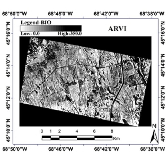
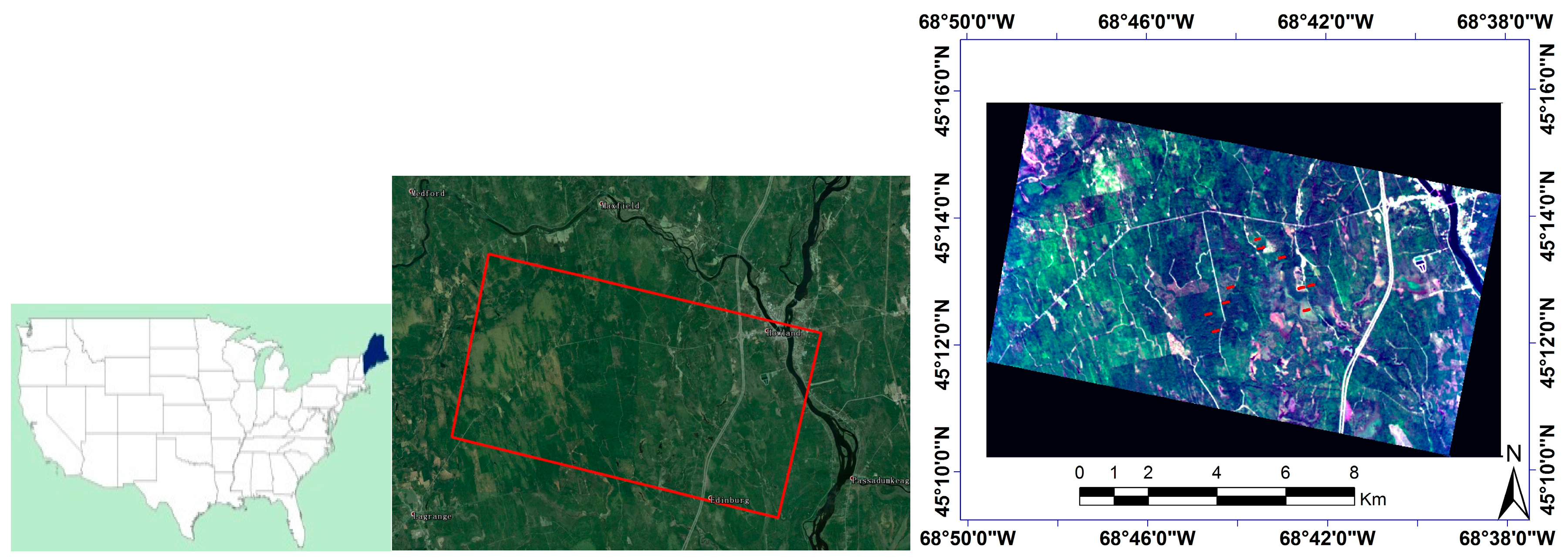
2.1. Study Site

In this paper, the study area is located in Howland, Maine, USA (45.17°N–45.26°N, 68.65°W–68.81°W), as shown in Figure 1. The forest of Howland has tremendous ecological value and plays host to researchers as a vital site in research on how forests remove carbon dioxide from the atmosphere and store it in plant biomass. The natural stands in this northern hardwood boreal transitional forest consist of hemlock–spruce–fir, aspen–birch, and hemlock–hardwood mixtures. Common species include quaking aspen, paper birch, eastern hemlock, red spruce, balsam fir, and red maple. The regional features are relatively level, where the elevation ranges from 20 m to 158 m within an area covered by the Compact High Resolution Imaging Spectrometer onboard the Project for On-board Autonomy (CHRIS/PROBA) data used in this study. Additionally, almost 450 ha of the surrounding area consist of bogs and other wetlands. Generally, the soils throughout the forest are glacial tills, acidic in reaction, with a low fertility and high organic composition. The climate is chiefly cold, humid, and continental. Summer maximum temperatures of 30 °C are common, and winter minimums can reach −30 °C. The mean annual air temperature (1996–2010) at Howland tower is 6.7 °C and average annual rainfall (1950–2000) is 1050 mm.

2.2. Field Samplings

Howland field measurements were conducted from 2009 to 2011 by the NASA Deformation, Ecosystem Structure and Dynamics of Ice (DESDynl) project. Twenty-four plots, measuring 1-ha (200 m × 50 m), were established in 2009 and 2010. Each plot was divided into neighboring 25 m × 25 m subplots, which can be aggregated into 96 subplots of 0.25-ha (50 m × 50 m). In total, 40 subplots were selected for testing the model after removing subplots outside of CHRIS image data, and the geographical locations are shown in Figure 1. In the paper the location of the sampling plots was measured using Real-time kinematic (RTK). For each subplot, Diameter at Breast Height (DBH, 1.3 m above ground), species, height of three highest trees, and typical tree crown information (crown width, live branch base height) were recorded. The biomass of subplots was calculated through the diameter-based allometric equations coming from the comprehensive report of USDA (United States Department of Agriculture) on North American forest given by Jenkins et al. [24]. Biomass was first calculated for each tree, and then total biomass was aggregated to subplot levels.

2.3. Satellite Data

The CHRIS sensor on PROBA provides spectral contiguous bands in the spectral wavelength range from 415 nm to 1050 nm, and a 17-m ground-sampling distance. PROBA is an experimental ESA space platform, which enables the sensor to capture images from five viewing angles. They were five CHRIS Fly-by Zenith Angles (FZA), namely: +36°, −36°, +55°, −55° and 0°. Five CHRIS modes were acquired for different observation tasks; CHRIS Mode 3 (Land) data were acquired over Howland. Data specifications are shown in Table 1, and the viewing geometry is shown in Figure 2. The sensor sweeps in the opposite direction, between two adjacent images, which results in the reversal of images of the Fly-by-Zenith Angle (FZA) ±36°, ±55° [25,26]; thus, it was rotated by the ENVI software. The swath effect of the images was eliminated using the official software, HDFclean, supplied by the European Space Agency (ESA). The geometric correction relied on ENVI orthorectification, considering the viewing geometry and geometric distortion due to the sensor, as well as the platform and topography, which used an ETM+ image from 23 August 2007, with a size of 28.5 × 28.5 m and a digital elevation model (DEM) of 1:50,000 [27].
The atmospheric correction of the CHRIS radiation data was performed using the fast line-of-sight atmospheric analysis of spectral hypercubes (FLAASH) model of ENVI, a MODerate resolution atmospheric TRANsmission (MODTRAN4)-based approach to remove scattering and absorption effects of atmosphere constituents for nadir and non-nadir viewing instruments, which enables the processing of data from tiled sensors by considering for varying path lengths through the atmosphere and varying transmittances. One distinct characteristic of this approach is that FLAASH is able to correct paths scattered by radiation and other adjacent effects. The surface reflectance generated by FLAASH represents BRDF through band response functions, imaging time, solar and sensor positions, and the location of the study area [28,29].

2.4. The Building of a Look-Up Table

The Look Up Table (LUT) database should include all kinds of combinations of environmental conditions and forest structures. Firstly, the forest growth model, ZELIG, is used to generate forest scenes, which are used to drive the Discrete Anisotropic Radiative Transfer (DART) model, as described in References [30,31]. ZELIG is an individual tree simulator that simulates the establishment, annual diameter growth, and mortality of each tree on an array of model plots. Table 2 shows the input parameters related to the growth and environmental response of the dominant tree species used in the Howland simulation. Because of the various random processes in the forest growth model, the ZELIG model runs five times to generate forest stands from 0 to 500 years with increments of five years. Secondly, from the forest stands, the parameters used as inputs for the DART model were determined, including tree species, tree location, height below crown, height within crown, diameter at breast height (BDH), crown type, crown height, crown geometry parameters, and leaf are index (LAI). The BRDF was simulated using the DART model and then the biomass was calculated using tree height and BDH.
The DART model was developed by the Center for the Study of the BIOsphere from Space, and simulates the radiation transfer in any complex 3D scene, using an innovative multispectral approach (ray tracing, exact kernel, and discrete ordinate techniques) over the entire optical domain [32]. The results are accurate; however, they demand a considerable number of calculations. The DART model simulates natural 3D forested scenes, and accurately reflects the effects of different factors on BRDF, which is affirmed by the international radiation transfer model intercomparison (RAMI3). In the calculation of forest BRDF, 29 local incidence angles from −70° to 70°, with 5° intervals, are used. The solar zenith angle was calculated using information from the CHRIS data. The main parameters are presented in Table 3.

2.5. Data Analysis

The following eight vegetation indices were selected for data analyses in order to represent forest structure and plant physiology, and are categorized into traditional VIs (1–6) and angle VIs (7–8) (Table 4). The equations and references are listed in Table 4. Because the reflectance properties of a land surface are anisotropic in nature, the vegetation indices are assumed to be sensitive to changing viewing angles, depending on the spectral bands used and the degree of surface anisotropy present in the observed scene [16]. Because forest surface anisotropy is affected by the canopy size, tree height, stands density, and shadow, there is a potential relationship between vegetation index and forest biomass. In the paper, the eight VIs were calculated using two types of reflectance, one from LUT and the other from CHRIS images. The pixels of the CHRIS images were selected according to the field measurement locations. CHRIS Land Mode 3 has 18 bands, and was categorized into four wavelength ranges: R BLUE (442 nm, 490 nm), R GREEN (530 nm, 551 nm, 570 nm), R RED (631 nm, 661 nm, 672 nm, 697 nm, 703 nm, 709 nm, 742 nm, 748 nm), and R NIR (781 nm, 872 nm, 895 nm, 905 nm, 1019 nm).
Firstly, in order to compare the off-nadir with the nadir, the six traditional VIs were calculated using the nadir angle reflectance from LUT, using the formula defined in Table 4, for example, the Simple Ratio Index (SRI) was calculated for 5 × 8 = 40 values. Then, the VIs were calculated using the 29 local incidence angle reflectances, the 29 angle reflectances can make up more than one value; for example, the SRI was calculated for 5 × 8 × 29 × 29 = 33,640 values, because there are five bands in the near infrared wavelength range and eight bands in the red wavelength range, and each band has 28 angles. The correlation coefficient (R) between the vegetation index and the biomass of LUT was calculated. RMSE (Root Mean Square Error) and rRMSE (Relative Root Mean Square Error) were calculated for each VI, rRMSE = RMSE / W i ^ ¯ , where W i ^ ¯ is average of W i ^ and W i ^ is the biomass estimated by a nonlinear regression model. According to the allometric functions and the nonlinear relationship between biomass and VIs, the following nonlinear regression model was used. lnY = A + BlnX , where Y is biomass, X is VIs, and A and B are coefficients. The minimum RMSE of SRI was determined and the corresponding wavelengths and angles from the 40 and 33,640 values were determined. Then, the ground measure biomass and CHRIS image data were used to calculate the five VIs, using the same method, in order to test the advantages of multi-angle remote sensing. The VIs, built by a sensitive angle and band, were used to calculate the corresponding A and B, and then the model was used to inverse the biomass. However, the two angle VIs, HDS and NDHD, were calculated using the same band and different angles, as defined in Reference [22].
Secondly, the correlation coefficient between BRDF and the biomass was calculated, based on the LUT, and 18 curves were calculated.
Thirdly, the VIs were calculated using the 29 angles from −70° to 70° with 5° intervals and 18 bands were used to find the sensitive angles and bands. For example, SRI was calculated to be 18 × 18 × 29 × 29 = 272,484 different values, R RED was not limited in the red wavelength range, and 18 bands × 29 angles = 522 values were determined, this was also the case for R NIR . The R correlation between each vegetation index and biomass was established and RMSE and rRMSE were calculated. The minimum RMSE of SRI was found, and the corresponding wavelength and angle from the 272,484 values was determined. The other VIs were processed using the same method, and then ground measure biomass and CHRIS image data were used to calculate the six VIs, using the same method. However, the two angle VIs, HDS and NDHD, have the same results as SRI and NDVI if calculated without the band limit, thus, the two VIs were not calculated again. This will help us to understand the viewing angle and the direction effects on biomass.

3. Results

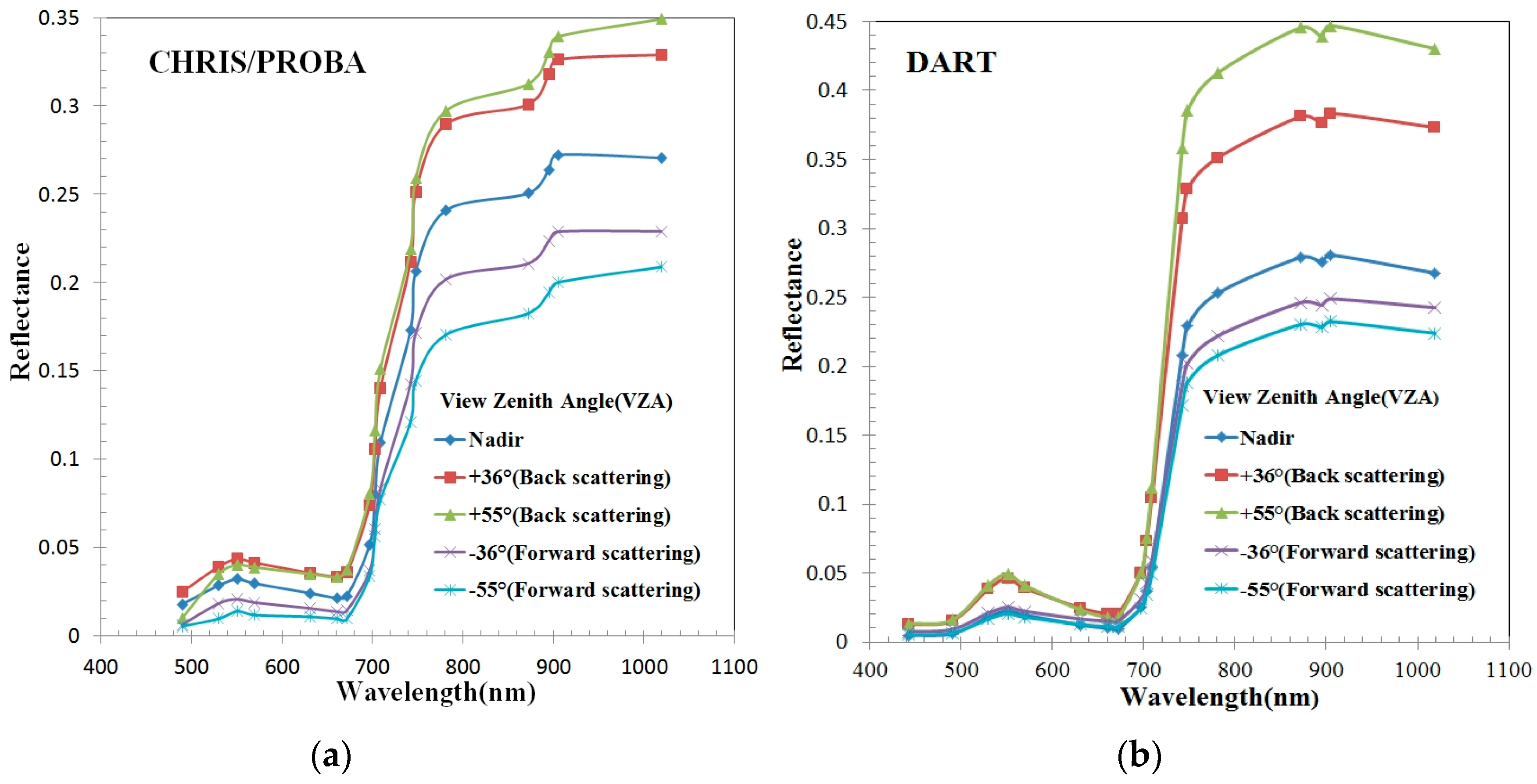
3.1. Comparison Nadir Angle with Off-Nadir Angle

In Table 5, every traditional vegetation index was calculated using the nadir angle and the off-nadir angle, as noted in the Comment column. The “Red/angle” represents the optimal red wavelength and angle when the RMSE is minimal. The results show that the off-nadir RMSE and rRMSE were reduced by an average of about 20% when compared with the nadir, and the greatest reduction is 64% for NDVI and 61% for ARVI. The R square was improved from 0.398 to 0.943 for ARVI. For the other two angle vegetation indices, HDS and NDHD, the RMSE and rRMSE were also very small, although not the minimum values. The off-nadir RMSE of eight VIs were smaller than the nadir, which shows that multi-angle remote sensing can reflect the three-dimensional structural information of forests and improve the accuracy of biomass retrieval, relative to the traditional single angle.
In order to prove the results, ground measure and CHRIS image data were used to find the optimal wavelength and angle, for both the nadir and off-nadir. In Table 6, the results show that, compared with the nadir, the off-nadir RMSE and rRMSE were reduced by an average of about 10%, and the maximum decrease is 23% for ARVI. The R square was also improved, from 0.612 to 0.697 for ARVI. The off-nadir RMSE of eight VIs were smaller than the nadir, and the result prove that multi-angle remote sensing can provide more structural information on forests than nadir angle observation.
In addition to the above-mentioned results, from Table 5 and Table 6 we can see the optimal wavelength focused on some bands, for example, in Table 5, the optimal red wavelengths are 709 nm and 703 nm, the optimal near-infrared wavelengths are 742 nm and 748 nm, and the optimal blue wavelengths are 490 nm and 442 nm. In Table 6, the optimal red wavelengths are 709 nm and 672 nm, the optimal near-infrared wavelengths are 742 nm and 748 nm, and the optimal blue wavelength is 490 nm. The results show that the structural information of forests is more sensitive to angle information. In order to test the results, the correlation coefficient between each band reflectance and biomass was calculated and are shown in Figure 3.

3.2. Band Effects on Biomass

From Table 5 and Table 6, we can see that the structural information of forests is more sensitive to angle information compared with band information. In order to test the results, the correlation coefficient between each band reflectance and biomass was calculated and are shown in Figure 3. In Figure 3, the horizontal axis is the view zenith angle and the vertical axis is the correlation coefficient between each band reflectance and biomass; the 18 curves represent the 18 bands of a CHRIS image. According to the curve shape, the 18 bands were separated into four groups. The curves in the near-infrared band group, of which the wavelengths are more than 709 nm, have a similar shape. The blue bands, 442 nm and 490 nm, have a similar shape, the green bands, 530 nm, 551 nm, and 709 nm have a similar shape, and the red bands, 631 nm, 661 nm, 972 nm, 697 nm, 703 nm, and 709 nm also have a similar shape. There is a great difference between the near infrared group and the other three groups, and, in the visible band group, the blue, green, and red band curves also have small differences. The correlations are much lower than the VIs; however, the highest correlations appear in the forward scattering direction (shadowed canopy) within the red band range. Because of the greater red reflectance dependence on its formulation when compared to the other indices, EVI showed sensitivity to view angle, view direction, and solar illumination. EVI has the highest R², as shown in Table 6.
There were greater reflectance differences in the CHRIS viewing directions in the NIR for Howland Forest (Figure 4a). Despite the differences in the magnitude of reflectance, results were generally consistent with the DART modeled spectra (Figure 4b). In both figures, the reflectance increased from the forward scattering to the backscattering, as expected, and the reflectance of each band within the four groups varied with angle, and is the same as is shown in Figure 4b, which can be tested to show that each group has a similar shape.

3.3. View-Illumination Effects on Biomass

The above-mentioned results highlight that view-illumination is the main factor effect BRDF value in the change of forest biomass, thus, the sensitive angle should been found in order to improve the accuracy of forest biomass retrieval. Then, six VIs were calculated using all angles and all bands, without limiting the band range, in considering the influence of the band and the results are shown in Table 7 and Table 8. In Table 7, LUT data were used, and, in Table 8, ground measure and CHRIS image data were used.
In order to compare Table 5 to Table 7, the RMSE and rRMSE of each VI were reduced, comparing the off-nadir with a limited band range with the off-nadir without limiting the band range. The greatest values are from 45.493 to 17.375 for PVI. The R square of each vegetation index was greater than 0.9. The results also show that multi-angle remote sensing can improve the accuracy of forest biomass retrieval. Table 7 also shows that the backward angles, 20°, 40°, 45°, and 60°, and the forward angles, −45°, −50°, −55°, −65°, and −70°, were found, and the most common backward angle value was 45° and the forward angles were –70° and –65°. These angles are the “hot” spot and “dark” spot angles, because the sun zenith angle is 44.3°. In addition, the vegetation index with the smallest RMSE is still ARVI, the angles of which are 45°, 60°, and −65°. In Table 5, the backward angles are 10°, 40°, 45°, and 70°, and the forward angles are −40°, −60°, −65°, and −70°, and the most common backward angle value is also 45°, and the forward angles are −70° and −65°. The present results implicate that the angles around the “hot” spot and the “dark” spot contain the main information about forest structure, and there was a maximum correlation relationship between them and forest biomass in Howland, where the tree species belong to coniferous forests and the forest structure is simple. However, in this paper, the results show that “hot” spots and “dark” spots should be combined in order to get better results and higher correlations with forest biomass. It is possible that the signal angle has a lower correlation with forest biomass.
The two angle VIs, HDS and NDHD, have the same results as SRI and NDVI if they are calculated without the band limit. In Table 7, HDS and NDHD were calculated using the different bands and different angles, and they have the same values as SRI and NDVI, respectively. The RMSE and rRMSE values were smaller than those calculated using same bands and different angles, which also show that the combination of sensitive angles and sensitive bands is suitable for forest biomass retrieval. The above-mentioned results were tested using a CHRIS image and field measured biomass, as shown in Table 8; the backward angles were 36° and 55°, which are around the “hot” spot angle, and the forward angle was –55°, which is around the “dark” spot angle, are the optimal angles.

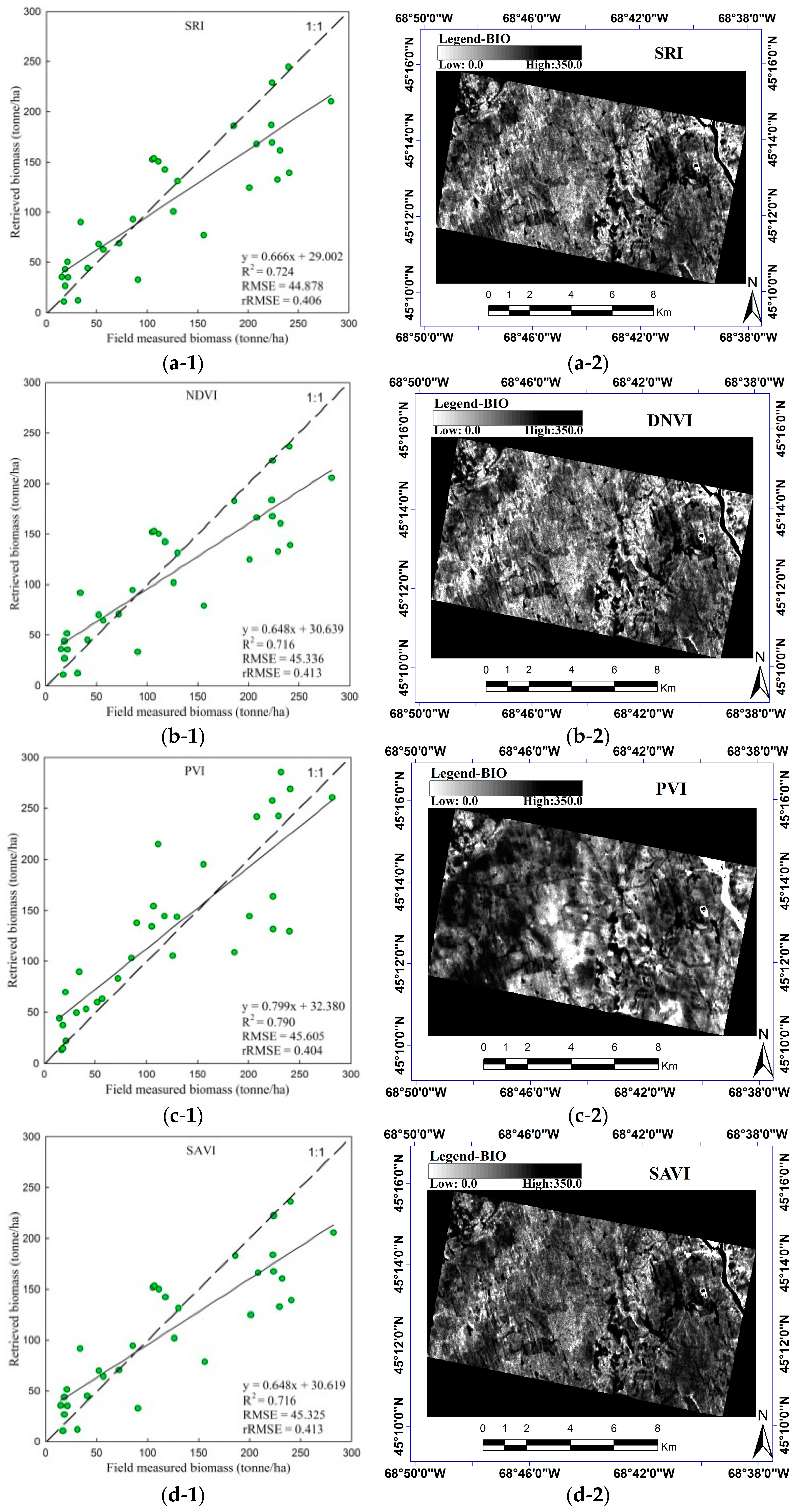
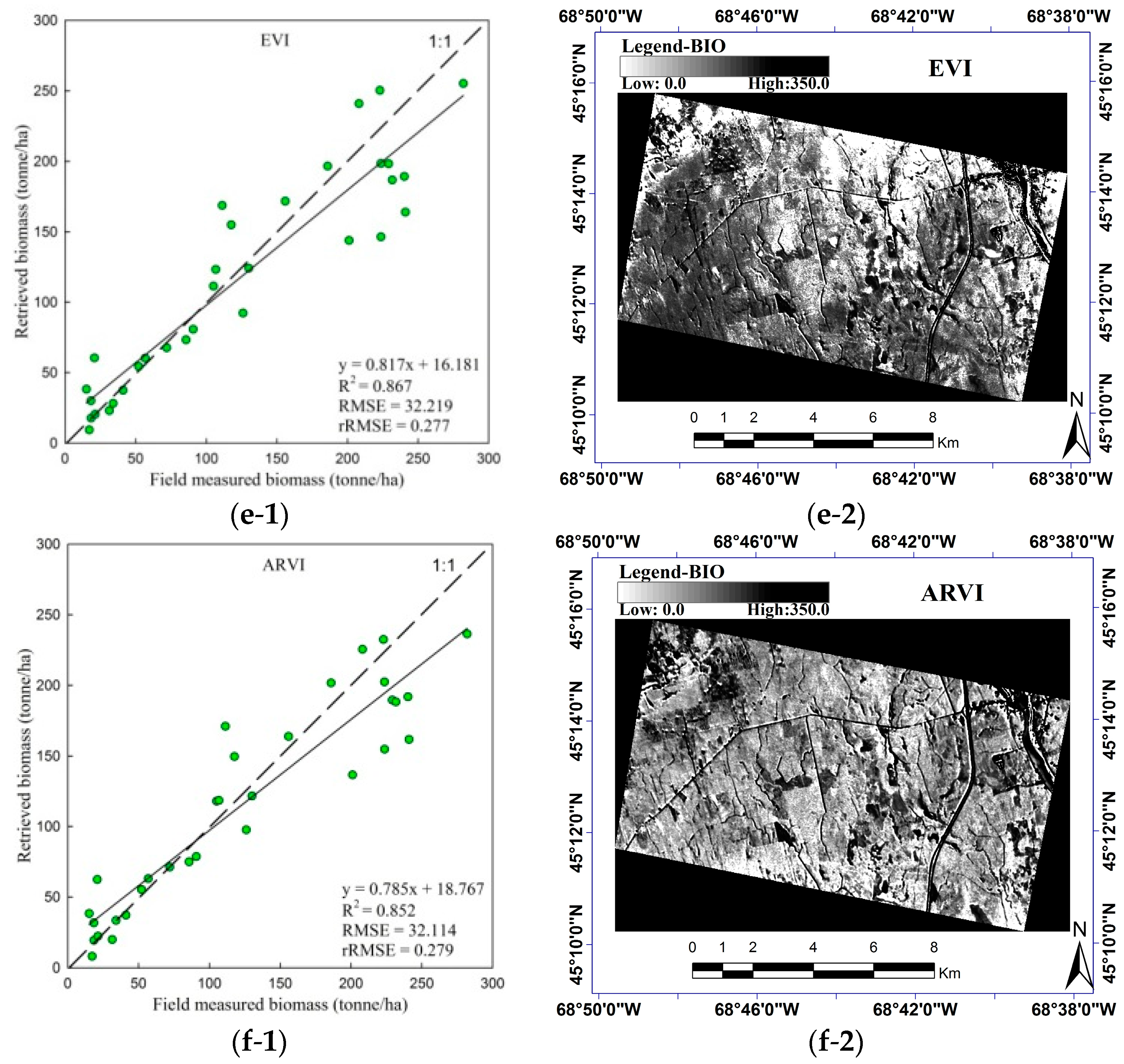
3.4. Biomass Estimation

From the scatter diagrams and biomass thematic maps of the six VIs in Figure 5, and the tables shown above, we found that ARVI is the best vegetation index to retrieval forest biomass from Howland. Because the points in the ARVI scatter diagrams are close to the dotted line, and the biomass thematic maps, are better for reflecting the actual forest distribution. The results are also shown in Table 4, Table 5, Table 6 and Table 7, and, in the four tables, the RMSEs and rRMSEs of ARVI are always minimal. However, the biomass inversion results tend to be over-estimate at lower values and under-estimate at higher one. It is important to note the reflectance values estimated from orbital data are explained by LAI and other structural parameters, but, as a tree grows, it accumulates biomass but LAI and others important structural data do not increase. Younger trees present higher LAI and lower biomass. When they are adult or mature, they present low LAI and high biomass. The VIs values are affected by LAI.

4. Discussion

Multi-angle remote sensing can provide more structural information regarding forests than nadir-angle observation. Compared with nadir angle observation, multi-angle can acquire some two-dimension images and then three-dimensional information can be extracted. The nadir image only provides one, two-dimension image, which loses the three-dimensional information.
Multiple scattering and shadowing are the main reasons that cause differences between the near-infrared and visible bands. The reflectance of leaf in NIR mainly depend on the inside structure of a cell, because the refraction index of a cell wall is high, which causes a high upward radiation energy. Because the chlorophyll in a leaf can perform photosynthesis, the reflectance is low in the red band [38]. Multiple scattering within canopies, among canopies, as well as between canopies and the background were increased [39]. A slight reflectance was observed in foliage and soil in the visible band, thus, the multiple scattering within canopies, among canopies, and between canopies and the background could be small.
However, in the visible band group, the blue, green, and red band curves also have small differences. As the effects of multiple scattering are the same for the visible band, there are other confounding factors affecting the relationship between BRDF and biomass, in addition to forest structure information. In the process of vegetation growth, not only does the forest three-dimensional structure change, but, also, the chemical composition and physical structure inside the tree components change, which cause blue, green, and red band curves to be of different shapes. This change also exists in the near infrared band. Some of chemical compositions include chlorophyll or carotenoid pigment levels [40]. The results show that the sensitive angle should be the main factor; at the same time, the effects of the bands should also be taken into account when the forest structure information is extracted using multi-angle remote-sensing data. However, considering orbital imagery, visible bands are also strongly influenced by shadowing. It is difficult to separate the influence of pigments and multiple shadowing, and the results aim to show that there is a primary relationship between angle and forest structures, such as biomass; however, there is a relationship between band and chemical composition that also vary in effects relative to biomass. Thus, the hope is to find a sensitive angle and suitable band in order to extract forest biomass.
The two VIs, PVI and SAVI, did not present well, because they were mainly influenced by soil background, and at the high angle of the viewed part of the ground is too small, near zero. Because view-illumination effects vary with canopy structure, angle is the key factor affecting the anisotropy of VIs determined from hyperspectral and multi-angle CHRIS/PROBA data. However, this is not the only factor that drives the VIs in Howland, in which the presence of within-canopy photosynthetic vegetation should be considered. Thus, there are other confounding factors, other than view-illumination effects, affecting the relationship between VIs and biomass. Some of them were reviewed by Middleton et al. (2011), and include chlorophyll and carotenoid pigments levels, and should be presented by different band reflectance [41].
The present results suggest that the angles around “hot” spots and “dark” spots contain the main forest structure information, and there were maximum correlation relationships between them and forest biomass in Howland. We also found that the angle values are greater, in several cases, and the optimal band/angle, with a minimum RMSE, occurs with a very high view geometry (70°). Thus, large view angles are suitable for extracting forest biomass. At a high view angle, more of the canopy can be seen and the viewed shadow and illumination canopy can include all of the vegetation information; however, the aerial proportions of the viewed ground are small. It may be reasonable to expect that the observed proportions of Photosynthetic Vegetation (PV) and Non-Photosynthetic Vegetation (NPV) depend on the viewing angle. For instance, it is likely that, at greater viewing angles, a lower proportion of PV and a greater proportion of NPV contribute to the observed canopy reflectance [16]. As the tree species of Howland are coniferous, the structure is simple. However, NPV includes canopy branches and twigs, which primarily make up canopy biomass, and there is a good relationship between canopy biomass and forest biomass [42].
Because vegetation and soil are composed of a complex non-Lambertian system, BRDF is a function of many variables, which include sensor viewing direction, solar radiation direction, geometric parameters (LAI, leaf angle distribution (LAD), canopy size, canopy spatial distribution and nelson foliage distribution, etc.), optical parameters (reflectance and transmittance of vegetation composition), etc. There is a direct relationship between some of the variables and forest biomass, which are called forest structural parameters. However, there is an indirect relationship between some of the variables and forest biomass, which are called forest non-structural parameters. Some variables are even unpredictable, such as LAD, of which the values are altered and does not only depend on forest scene, species, and growing season, but also change due to wind, plant diseases, and man-made factors. Obviously, single-band reflectance is greatly different due to changes to any single factor; thus, we need to use two or more wavelengths in order to reduce the influence on BRDF. Subtracting the different angle reflectance can highlight the structure information of a forest canopy, and dividing can reduce the influence of non-forest structure on BRDF. Therefore, ARVI, calculated by combining sensitive angles with sensitive bands, was suitable for retrieving forest biomass, and the RMSE value is minimal, which evolves based on NDVI and can reduce the influence of aerosol. The result show that the vegetation index, using three different angles, can extract the most forest structure information in Howland, and, further, it will improve the accuracy of forest biomass retrieval.

5. Conclusions

In this paper, we prove that multi-angle remote sensing can extract the biomass information of a forest via observation from different directions, and improves the accuracy of biomass retrieval compared with traditional single-angle remote sensing. The paper investigated how to determine the sensitive angle and band in order to build optimal angle vegetation indices for forest biomass retrieval. We have used ZELIG and DART models to simulate the BRDF of a forest canopy, and built a LUT for determining the sensitive angle and band; further, multi-angle CHRIS/PROBA data and field-measured biomass were used to test the results. We found that the reflectance around hot spots and dark spots include the main biomass information of a forest canopy, because the greater angle viewing is sensitive to non-photosynthetic leaf activity in a canopy (e.g., branches, trunks), which make up canopy biomass, and also has good relationship with forest biomass [43]. Crown size is considered to be one of the most important traits that affect radial tree growth, and because there is a relationship between canopy biomass and forest biomass [44]. The greater angle also reduces the influence of noise reflectance from the ground. The results also show that this mainly does not happen in the cold spot direction compared with hot spot direction; the hot spots included the main biomass information. However, the “hot” spot and “dark” spot should be combined in order to get better results and higher correlations with forest biomass. In addition, the signal angle may have a lower correlation with forest biomass. At a high view angle, the greater part of the canopy can be seen, and the viewed shadow and illumination canopy can include most of the vegetation information; however, the aerial proportions of the viewed ground are small.
Hence, the difference in the reflectance around a hot spot at different wavelength is normalized against that of a dark spot at different wavelength, and this accentuates the importance of canopy geometry on the new angle indices, and also takes into account of the influence of leaf optical properties on forest biomass. During the process of vegetation growth, as the biomass changes, not only does the forest’s biophysical structure change, but also the forest’s biochemical composition changes, which leads to changes in the reflectance of forest composition.
Finally, the authors presented a new and optimal angle vegetation index to retrieve the forest biomass from bidirectional signatures, based on the traditional vegetation index, ARVI, which is made of three bands with three directions. The results show that more than two bands can highlight forest biomass information and reduce the influence of other non-structural parameters on BRDF. The potential of forest biomass retrieval, based on angle vegetation indices using CHRIS/PROBA data, investigate how to take advantage of the implied information of BRDF; in particular, the two paramount directional signatures, which are around maximum (hot spot) and minimum (dark spot) reflectances. In this respect, the feasibility of retrieving the structural properties of vegetation from different satellite observations is a challenge. The POLarization and Directionality of the Earth's Reflectance onboard the Advanced Earth Observing Satellite (POLDER/ADEOS) mission fosters such an investigation, as it was shown that the angle effect is a major feature of BRDF in terrestrial biomes [45].

Acknowledgments

The research undertaken for this paper was funded by National Program on Key Basic Research Project-973 Program(Grant No. 2013CB733404),the National Natural Science Foundation of China (Grant No. 41471311, 41201435), Spatial Geography Information Laboratory Open Fund(Grant No. KJKF-12-02).

Author Contributions

Qiang Wang and Yong Pang conceived and designed the idea of paper; Zengyuan Li and Guoqing Sun performed the experiments; Erxue Chen, Wenge Ni-Meister contributed analysis methods and tools; Qiang Wang analyzed the data and wrote the paper.

Conflicts of Interest

The authors declare no conflict of interest.

References

  1. Kimes, D.S.; Ranson, K.J.; Sun, G.Q.; Blair, J.B. Predicting lidar measured forest vertical structure from multi-angle spectral data. Remote Sens. Environ. 2006, 100, 503–511. [Google Scholar] [CrossRef]
  2. Jenkins, J.C.; Chojnacky, D.; Heath, L.S.; Birdsey, R.A. Comprehensive Database of Diameter-Based Biomass Regressions for North American Tree Species; General Technical Report NE-319; U.S. Department of Agriculture, Forest Service, Northeastern Research Station: Newtown Square, PA, USA, 2004; p. 45.
  3. Tritton, L.M.; Hornbeck, J.W. Biomass Equations for Major Tree Species of the Northeast; General Technical Report NE-69; U.S. Department of Agriculture, Forest Service, Northeastern Forest Experiment Station: Newtown Square, PA, USA, 1982; p. 46.
  4. Ni, W.J.; Sun, G.Q.; Ranson, K.J.; Zhang, Z.Y.; He, Y.T.; Huang, W.L.; Guo, Z.F. Model based analysis of the influence of forest structures on the scattering phase center at L-band. IEEE Trans. Geosci. Remote Sens. 2014, 52, 3937–3946. [Google Scholar]
  5. Pang, Y.; Li, Z.Y. Inversion of biomass components of the temperate forest using airborne Lidar technology in Xiaoxing’an Mountains, Northeastern of China. Chin. J. Plant Ecol. 2012, 36, 1095–1105. [Google Scholar] [CrossRef]
  6. Lefsky, M.A.; Cohen, W.B.; Parker, G.G.; Harding, D.J. Lidar remote sensing for ecosystem studies. Bioscience 2002, 52, 19–30. [Google Scholar] [CrossRef]
  7. Wulder, M. Optical remote sensing techniques for the assessment of forest inventory and biophysical parameters. Proc. Phys. Geogr. 1998, 22, 449–476. [Google Scholar] [CrossRef]
  8. Wang, Q.; Pang, Y.; Li, Z.Y.; Chen, E.X.; Sun, G.Q.; Tan, B.X. Improvement and application of the conifer forest multiangular hybrid GORT Model-MGeoSAIL. IEEE Trans. Geosci. Remote Sens. 2013, 51, 5047–5059. [Google Scholar] [CrossRef]
  9. Leroy, M.; Roujean, J.L. Sun and view angle corrections on reflectances derived from NOAA/AVHRR data. IEEE Trans. Geosci. Remote Sens. 1994, 32, 684–697. [Google Scholar] [CrossRef]
  10. Asner, G.P. Contributions of multi-view angle remote sensing to land surface and biogeochemical research. Remote Sens. Rev. 2000, 18, 137–162. [Google Scholar] [CrossRef]
  11. Asner, G.P.; Braswell, B.H.; Schimel, D.S.; Wessman, C.A. Ecological research needs from multi-angle remote sensing data. Remote Sens. Environ. 1991, 63, 155–165. [Google Scholar] [CrossRef]
  12. Diner, D.J.; Asner, G.P.; Davies, R.; Knyazikhin, Y.; Muller, J.P.; Nolin, A.W.; Pinty, B.; Schaaf, C.B.; Stroeve, J. New directions in Earth observing: scientific application of multi-angle remote sensing. Bull. Am. Meteorol. Soc. 1999, 80, 2209–2228. [Google Scholar] [CrossRef]
  13. Sandmeier, S.; Deering, D.W. Structure analysis and classification of boreal forests using hyper-spectral BRDF data from ASAS. Remote Sens. Environ. 1999, 69, 281–295. [Google Scholar] [CrossRef]
  14. Kimes, D.S.; Nelson, R.F.; Manry, M.T.; Fung, A. Attributes of neural networks for extracting continuous vegetation variables from optical and radar measurements. Int. J. Remote Sens. 1998, 19, 2639–2663. [Google Scholar] [CrossRef]
  15. Myneni, R.B.; Maggion, S.; Iaquinto, J.; Privette, J.L.; Gobron, N.; Pinty, B.; Kimes, D.S.; Verstraete, M.M.; Williams, D.L. Optical remote-sensing of vegetation-modeling, caveats, and algorithms. Remote Sens. Environ. 1995, 51, 169–188. [Google Scholar] [CrossRef]
  16. Verrelst, J.; Schaepman, M.E.; Koetz, B.; Kneubühlerb, M. Angular sensitivity analysis of vegetation indices derived from CHRIS/PROBA data. Remote Sens. Environ. 2008, 112, 2341–2353. [Google Scholar] [CrossRef]
  17. Jackson, R.D.; Teillet, P.M.; Slater, P.N.; Fedosejevs, G.; Jasinski, M.F.; Aase, J.K.; Moran, M.S. Bidirectional measurements of surface reflectance for view angle corrections of oblique imagery. Remote Sens. Environ. 1990, 32, 189–202. [Google Scholar] [CrossRef]
  18. Pinter, P.J.; Zipoli, G.; Maracchi, G.; Reginato, R.J. Influence of topography and sensor view angles on NIR/red ratio and greenness vegetation indices of wheat. Int. J. Remote Sens. 1987, 8, 953–957. [Google Scholar] [CrossRef]
  19. Roberts, D.A.; Roth, K.L.; Perroy, R.L. Chapter 14. Hyperspectral vegetation indices. In Hyperspectral Remote Sensing of Vegetation; Thenkabail, P.S., Lyon, J.G., Huete, A., Eds.; CRC Press, Taylor and Francis Group: Boca Raton, FL, USA, 2011; pp. 309–327. [Google Scholar]
  20. Garbulsky, M.F.; Penuelas, J.; Gamon, J.; Inoue, Y.; Filella, I. The Photochemical Reflectance Index (PRI) and the remote sensing of leaf, canopy and ecosystem radiation use efficiencies: A review and meta-analysis. Remote Sens. Environ. 2011, 115, 281–297. [Google Scholar] [CrossRef]
  21. Huete, A.R.; Kim, Y.; Ratana, P.; Didan, K.; Shimabukuro, Y.E.; Miura, T. Chapter 11. Assessment of phenologic variability in Amazon tropical rainforests using hyperspectral Hyperion and MODIS satellite data. In Hyperspectral Remote Sensing of Tropical and Sub-tropical Forests; Kalacska, M., Anchez-Azofeifa, G.A., Eds.; CRC Press, Taylor and Francis Group: Boca Raton, FL, USA, 2008; pp. 233–259. [Google Scholar]
  22. Chen, J.M.; Liu, J.; Leblanc, S.G.; Lacaze, R.; Roujean, J.L. Multi-angular optical remote sensing for assessing vegetation structure and carbon absorption. Remote Sens. Environ. 2003, 84, 516–525. [Google Scholar] [CrossRef]
  23. Wu, C.Y.; Niu, Z.; Wang, J.D.; Gao, S.; Huang, W.J. Predicting leaf area index in wheat using angular vegetation indices derived from in situ canopy measurements. Can. J. Remote Sens. 2010, 36, 301–312. [Google Scholar] [CrossRef]
  24. Jenkins, J.C.; Chojnacky, D.C.; Heath, L.S.; Birdsey, R.A. National-scale biomass estimators for United States tree species. Forest Sci. 2003, 49, 12–35. [Google Scholar]
  25. Barnsley, J.M.; Settle, J.J.; Cutter, M.A.; Lobb, D.R. The PROBA/CHRIS mission: A low-cost smallsat for hyperspectral multi-angle observations of the earth surface and atmosphere. IEEE Trans. Geosci. Remote Sens. 2004, 42, 1512–1520. [Google Scholar] [CrossRef]
  26. Guanter, L.; Alonso, L.; Moreno, J. A method for the surface reflectance retrieval from PROBA/CHRIS data over land: Application to ESA SPARC campaigns. IEEE Trans. Geosci. Remote Sens. 2005, 43, 2907–2917. [Google Scholar] [CrossRef]
  27. Kneubühler, M.; Kötz, B.; Richter, R.; Schaepman, M.; Ltten, K. Geimetric and radionmetric pre-processing of CHRIS/PROBA over mountainous terrain. In Proceedings of the 3rd CHRIS/PROBA Workshop, Frascati, Italy, 21–23 March 2005; pp. 59–64.
  28. Verrelst, J.; Clevers, J.G.P.; Schaepman, M.E. Merging the Minnaert-k parameter with spectral unmixing to map forest heterogeneity with CHRIS/PROBA data. IEEE Trans. Geosci. Remote Sens. 2010, 48, 4014–4022. [Google Scholar]
  29. Chan, J.C.W.; Ma, J.; van de Voorde, T.; Canters, F. Preliminary results of superresolution-enhanced angular hyperspectral (CHRIS/PROBA) images for land-cover classification. IEEE Trans. Geosci. Remote Sens. 2011, 8, 1011–1015. [Google Scholar] [CrossRef]
  30. Urban, D.L.; Bonan, G.B.; Smith, T.M.; Shugart, H.H. Spatial applications of gap models. Forest Ecol. Manag. 1991, 42, 95–110. [Google Scholar] [CrossRef]
  31. Gastellu-Etchegorry, J.P. DART User Manual. 2015. Available online: http://www.cesbio.upstlse.fr/dart/license/documentationsDart/DART_User_Manual.pdf (accessed on 27 October 2016).
  32. Gastellu-Etchegorry, J.P.; Martin, E.; Gascon, F. DART: A 3-D model for simulating satellite images and studying surface radiation budget. Int. J. Remote Sens. 2004, 25, 73–96. [Google Scholar] [CrossRef]
  33. Tucker, C.J. Red and photographic infrared linear combinations for monitoring vegetation. Remote Sens. Environ. 1979, 8, 127–150. [Google Scholar] [CrossRef]
  34. Richardson, A.J.; Everitt, J.H. Using spectral vegetation indices to estimate rangeland productivity. Geocarto Int. 1992, 7, 63–77. [Google Scholar] [CrossRef]
  35. Huete, A.R. A Soil-Adjusted Vegetation Index (SAVI). Remote Sens. Environ. 1988, 25, 295–309. [Google Scholar] [CrossRef]
  36. Huete, A.R.; Didan, K.; Miura, T.; Rodriguez, E.P.; Gao, X.; Ferreira, L.G. Overview of the radiometric and biophysical performance of the MODIS vegetation indices. Remote Sens. Environ. 2002, 83, 195–213. [Google Scholar] [CrossRef]
  37. Kaufman, Y.J.; Tanre, D. Atmospherically resistant vegetation index (ARVI) for EOS-MODIS. IEEE Trans. Geosci. Remote Sens. 1992, 30, 261–270. [Google Scholar] [CrossRef]
  38. Fang, X.Q.; Zhang, W.C. The application of remotely sensed data to the estimation of the leaf area index. Remote Sens. Land Res. 2003, 57, 58–62. [Google Scholar]
  39. Chen, J.M.; Leblanc, S.G. Multiple-scattering scheme useful for geometric optical modeling. IEEE Trans. Geosci. Remote Sens. 2001, 39, 1061–1071. [Google Scholar] [CrossRef]
  40. Galvao, L.S.; Breunig, F.M.; dos Santos, J.R.; de Moura, Y.M. View-illumination effects on hyperspectral vegetation indices in the Amazonian tropical forest. Int. J. Appl. Earth Obs. Geoinf. 2013, 21, 291–300. [Google Scholar] [CrossRef]
  41. Middleton, E.M.; Huemmrich, K.F.; Cheng, Y.; Margolis, H.A. Chapter 12. Spectral bioindicators of photosynthetic efficiency and vegetation stress. In Hyperspectral Remote Sensing of Vegetation; Thenkabail, P.S., Lyon, J.G., Huete, A., Eds.; CRC Press, Taylor and Francis Group: Boca Raton, FL, USA, 2011; pp. 265–288. [Google Scholar]
  42. Mäkelä, A.; Valentine, H.T. Crown ration influences allometric scaling in trees. Ecology 2006, 87, 2967–2972. [Google Scholar] [CrossRef]
  43. Vauhkonen, J.; Holopainen, M.; Kankare, V.; Vastaranta, M.; Viitala, R. Geometrically explicit description of forest canopy based on 3D triangulations of airborne laser scanning data. Remote Sens. Environ. 2016, 173, 248–257. [Google Scholar] [CrossRef]
  44. Fichtner, A.; Sturm, K.; Rickert, C.; Oheimb, G.; Härdtle, W. Crown size-growth relationships of European beech (Fagus sylvatica L.) are driven by the interplay of disturbance intensity and inter-specific competition. Forest Ecol. Manag. 2013, 302, 178–184. [Google Scholar] [CrossRef]
  45. Lacazea, R.; Chen, J.M.; Roujeana, J.L.; Leblanc, S.G. Retrieval of vegetation clumping index using hot spot signatures measured by POLDER instrument. Remote Sens. Environ. 2002, 79, 84–95. [Google Scholar] [CrossRef]
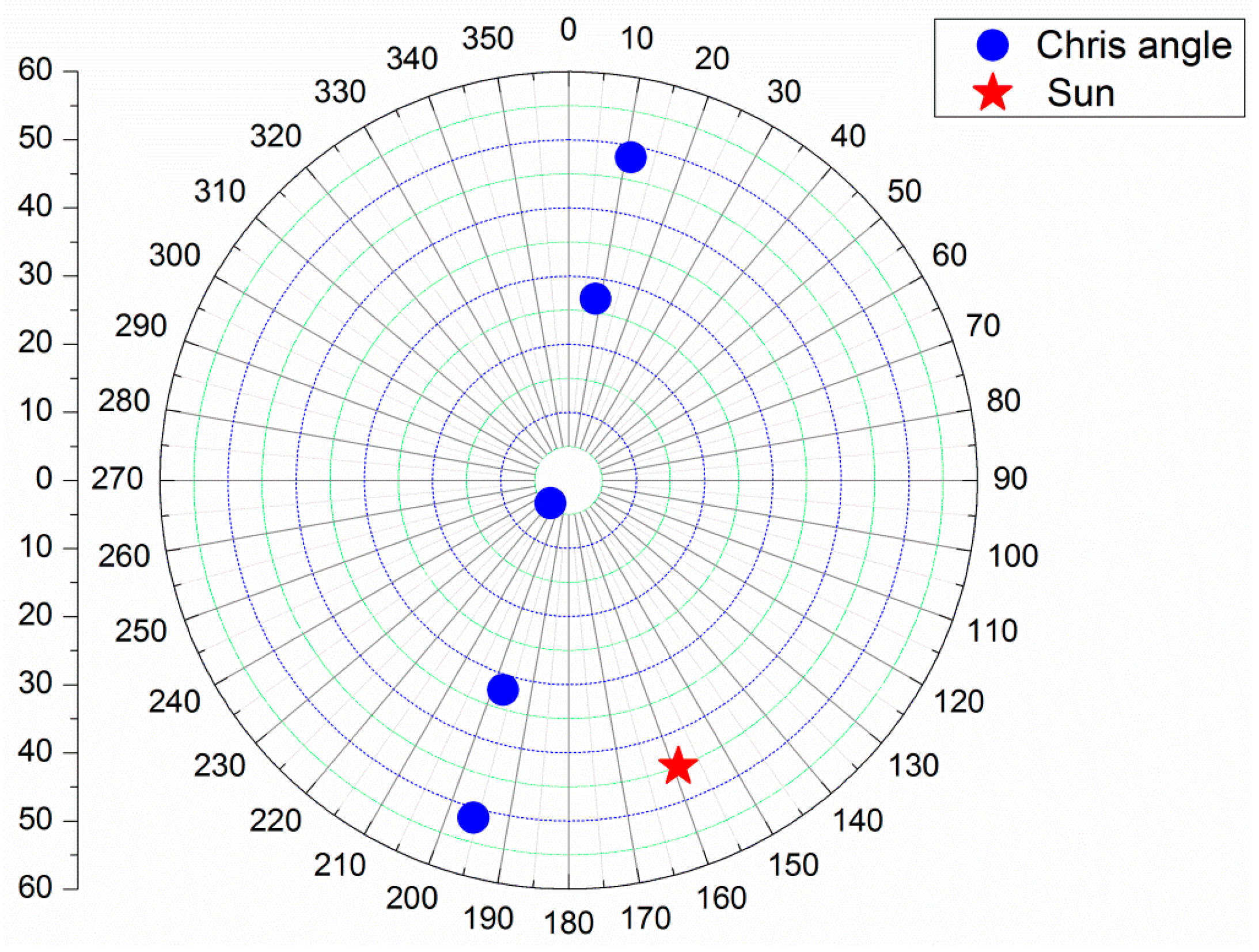
Figure 1. The spatial coverage of CHRIS data used in the Howland study area, and the geographical locations of field samplings (red square).
Remotesensing 08 00891 g001
Figure 2. Polar plot of the CHRIS image-viewing geometry.
Remotesensing 08 00891 g002
Figure 3. Correlation coefficients between all band reflectances and biomass.
Remotesensing 08 00891 g003
Figure 4. (a) Measured CHRIS/PROBA reflectance spectra; (b) simulated DART reflectance spectra of Howland for CHRIS/PROBA view zenith angles and directions.
Remotesensing 08 00891 g004
Figure 5. The performance of biomass inversion using six VIs, combining all angles with all bands in Table 8. (a-1) a scatter diagram comparing the measured biomass with the inversion biomass using SRI, and (a-2) the inversion biomass thematic map using SRI; (b-1,b-2) are for NDVI; (c-1,c-2) are for PVI; (d-1,d-2) are for SAVI; (e-1,e-2) are for EVI; (f-1,f-2) are for ARVI.
Remotesensing 08 00891 g005aRemotesensing 08 00891 g005b
Table 1. CHRIS specifications.
Study AreaImage AreaSamplingCentral Latitude and LongitudeViewing AnglesSpectral BandsSun ZenithSun Azimuth
Howland14 × 14 km
(744 × 748 pixels)
17 × 17 m @
662 km altitude
42°2′24′′
127°47′24′′
5 nominal angles @
−55°, −36°, 0°, +36°, +55°
18 bands, 442~1019 nm with 6~11 nm width44.3°159°
Table 2. Input parameters of growth and environmental response of dominant tree species used in the ZELIG simulation.
SpeciesAmaxDmaxHmaxGDDminDDmaxLightDrtNutri
aspen1506025004008002300522
birch15060300040010003000522
spruce3001103300605501800153
fir200703000505001800151
Amax: Maximum age, Dmax: Maximum diameter at breast height (cm), Hmax: Maximum height(m), G: Growth rate scaling coefficient, DDmin and DDmax: Minimum and maximum growing degree-days (5.56o base), Light: Shade-tolerance class (rank: 1 = very shade tolerant, 5 = very intolerant), Drt: Drought tolerance (rank: 1 = very drought-intolerant, 5 = very drough-tolerant), Nutri: Soil fertility response class (1 = nutrient stress intolerant, 3 = tolerant).
Table 3. Parameters of the look-up table.
ParametersRangeComments
Solar zenith44.3°The same as CHRIS data
View zenith0°–70°5° interval
Azimuth angle0°, 180°Principal and vertical plane
Bands18 bandsThe same as CHRIS data
Mean tree height3.25–16.93 (m)From Zelig model
Leaf area index0.13–9.7From Zelig model
Biomass0.166–41.694 (ton/ha)From Zelig model
Table 4. Eight Hyperion-derived vegetation indices used in the study.
Vegetation IndexFormulaDescriptionReference
Traditional vegetation index
SRI
Simple Ratio Index
R NIR / R RED Measure of green vegetation cover.Tucker (1979) [33]
NDVI
Normalized Difference Vegetation Index
( R NIR R RED ) / ( R NIR + R RED ) Measure of green vegetation cover.Tucker (1979)
PVI
perpendicular vegetation index
( R NIR aR RED b ) ( 1 + a 2 )
where a = 0.96916, b = 0.084726, and L = 0.5
To deduce information about soil surface conditions based on soil background lineRichardson and Everitt (1992) [34]
SAVI
A soil-adjusted vegetation index
( R NIR R RED ) ( 1 + 0.5 ) ( R NIR + R RED + 0.5 ) Similar as NDVI while correcting for high soil reflectanceHuete (1988) [35]
EVI
Enhanced Vegetation Index
2.5 ( ( R NIR R RED ) ( R NIR + 6 R RED 7.5 R BLUE + 1 ) ) More sensitive to plant canopy differences and reduce the influence of atmospheric conditionsHuete et al. (2002) [36]
ARVI
Atmospherically Resistant Vegetation Index
( R NIR ( 2 R RED R BLUE ) ) ( R NIR + ( 2 R RED R BLUE ) ) Similar as NDVI while being less sensitive to aerosol effectsKaufman and Tanre (1992) [37]
Angle vegetation index
HDS
Hot spot–Dark Spot index
( R HS R DS ) / R DS Measure of plant canopy structure informationChen et al., (2003) [20]
NDHD
Normalized Difference between Hot spot and Dark spot
( R HS R DS ) / ( R HS + R DS ) Measure of plant canopy structure information while reduce the influence of leaf optical propertiesChen et al., (2003)
Table 5. Comparison of nadir with off-nadir using the LUT.
R SquareRed/AngleNear-Infrared/AngleBlue/AngleRMSErRMSEComment
SRI0.880709/70742/45 27.7320.236off-nadir
0.327709/0905/0 46.6440.419nadir
NDVI0.956709/−65748/45 16.8500.142off-nadir
0.450709/0872/0 45.1220.340nadir
PVI0.823709/−70742/45 34.1410.287off-nadir
0.045709/0872/0 52.6810.505nadir
SAVI0.834709/−70742/40 35.4520.295off-nadir
0.114709/0872/0 50.9220.481nadir
EVI0.654709/−55742/55442/−5540.7830.349off-nadir
0.131709/0872/0442/050.4340.474nadir
ARVI0.943703/−70742/45490/−6518.6110.157off-nadir
0.398709/0872/0490/045.3040.404nadir
HDS0.931709/−40
709/45
21.0700.176off-nadir
NDHD0.893709/40
709/10
24.2750.203off-nadir
Table 6. View-illumination effects for the nadir with the off-nadir angle, using ground measures and CHRIS data.
R SquareRed/AngleNear-Infrared/AngleBlue/AngleRMSErRMSEComment
SRI0.712 672/−36748/−36 54.5180.482off-nadir
0.651 672/0742/0 57.9290.534nadir
NDVI0.643 672/−36742/−55 55.9260.535off-nadir
0.551 697/0742/0 61.5700.599nadir
PVI0.312 709/55742/0 76.0470.761off-nadir
0.232 709/0742/0 79.7760.843nadir
SAVI0.643 672/−36742/−55 55.9320.535off-nadir
0.551 697/0742/0 61.5730.599nadir
EVI0.724 672/−36742/−36490/–3647.1480.434off-nadir
0.677 672/0742/0490/052.919 0.489nadir
ARVI0.697 672/−36742/−55490/5545.4270.421off-nadir
0.612672/0742/0490/058.6630.565nadir
HDS0.572672/−36
672/55
57.0180.527off-nadir
NDHD0.618672/36
672/−36
59.3680.542off-nadir
Note: Wavelength unit is nanometer, angle unit is degrees.
Table 7. Optimal bands and angles using LUT.
R SquareRed/AngleNear-Infrared/AngleBlue/AngleGreen/AngleRMSErRMSE
SRI0.958709/−70781/45 15.9400.135
NDVI0.958 748/45 551/−6516.4320.139
PVI0.945709/−45 442/20 17.3750.147
SAVI0.910 490/−55570/−5018.7340.158
EVI0.941709/45
709/−70
551/4016.0030.135
ARVI0.964 781/45
781/60
551/−6514.6540.133
Note: Wavelength unit is nanometers, angle unit is degrees.
Table 8. Optimal bands and angles using ground measure and a CHRIS image.
R SquareRed/AngleNear-Infrared/AngleBlue/AngleGreen/AngleRMSErRMSE
SRI0.724697/36 570/3644.8780.406
NDVI0.716697/36 570/3645.3360.413
PVI0.790 781/55
1019/55
45.6050.404
SAVI0.716697/36 570/3645.3250.413
EVI0.867697/55 490/–55530/5532.2190.277
ARVI0.852697/55 490/–55530/5532.1140.279
Note: Wavelength unit is nanometer, angle unit is degrees.

