Urban–Rural Contrasts in Central-Eastern European Cities Using a MODIS 4 Micron Time Series

Abstract

A primary impact of urbanization on the local climate is evident in the phenomenon recognized as the Urban Heat Island (UHI) effect. This urban thermal anomaly can increase the health risks of vulnerable populations to heat waves. The surface UHI results from emittance in the longer wavelengths of the thermal infrared; however, there are also urban anomalies that are detectable from radiance in the shorter wavelengths (3–5 micron) of the Middle Infrared (MIR). Radiance in the MIR can penetrate urban haze which frequently obscures urban areas by scattering visible and near infrared radiation. We analyzed seasonal and spatial variations in MIR for three Central European cities from 2003 through 2012 using Moderate Resolution Imaging Spectrometer (MODIS) band 23 (~4 micron) to evaluate whether MIR radiance could be used to characterize heat anomalies associated with urban areas. We examined the seasonality of MIR radiance over urban areas and nearby croplands and found that the urban MIR anomalies varied due to time of year: cropland MIR could be larger than urban MIR when there was more exposed soil at planting and harvest times. Further, we compared monthly mean MIR with the Normalized Difference Vegetation Index (NDVI) to analyze contrasts between urban and rural areas. We found that the seasonal dynamic range of the MIR could exceed that of the NDVI. We explored the linkage between meteorological data and MIR radiance and found a range of responses from strong to weak dependence of MIR radiance on maximum temperature and accumulated precipitation. Our results extend the understanding of the anomalous characteristics of urban areas within a rural matrix.

1. Introduction

Among the many transformational anthropogenic activities, perhaps the most striking human impact on the global biosphere is the transformation of Earth’s land surface into urban areas [1]. This land cover conversion affects a wide range of processes, including the surface radiation and energy budgets, the water, carbon, and nutrient cycles, soil dynamics, vegetation productivity and phenology, and local and regional biotic diversity [2]. A primary impact of urbanization is on the local climate at multiple temporal scales. The structure of the urban built environment shows increased impervious surface area and more aboveground mass with higher thermal storage capacity than rural environments. Buildings, roofs, parking lots, and roads increase run-off, decrease evapotranspiration, and store absorbed sunlight and re-radiate it as heat, thereby increasing sensible heat flux. Thus, urban areas are usually warmer than nearby rural areas, a phenomenon recognized as the Urban Heat Island (UHI) effect [3,4]. Studies have shown that the environmental impacts of urban areas can extend well beyond administrative boundaries [5,6], and urban heat islands can increase the health risk of vulnerable populations to heat waves [7]. Intensity of the UHI effect depends on many factors, including building density, height, and arrangement; thermal and reflective properties of construction, paving, and roofing materials structures; size and arrangement of green spaces within the city; local and regional wind fields; season and time of year; and recent weather [7,8]. The UHI has been primarily characterized by near surface air temperature measurements and by remote sensing of the land surface temperature using thermal infrared sensors [9,10,11,12,13,14,15].

What constitutes the extent of an urban area is often not an easy question to answer, particularly in rapidly developing cities where administrative boundaries may not capture informal settlements or recent growth. Indeed, estimates of global urban area using remote sensing data range widely from 0.27 to 3.52 milion km² [15], due to various definitions of the urban area and the sensors and techniques for urban areas identification [16]. For many decades, researchers have measured differences in air temperatures at “urban” and “rural” sites to assess the magnitude of the UHI effect in specific cities [4,17]. Many methods of classification were developed. However, none of them was designed to classify field sites in recognition of the heat island effect [18]. To address this shortcoming, a new protocol, based on medium (30–100 m) resolution remote sensing data, has been proposed [18]. The combination of building types and land cover types creates distinct Local Climate Zones that promise to enable standardization and facilitate the exchange of urban temperature observations [18]. However, medium-resolution data have only been available at a resolution of 8–16 days, at best, or several weeks due to cloud cover [19], in contrast to lower spatial resolution data for which temporal resolution may be daily. In addition to cloudiness, anthropogenic aerosols from combustion sources complicate remote sensing analyses by enhancing the scattering of visible and near infrared wavelengths.

The Middle Infrared (MIR) region of the electromagnetic spectrum spans 3–5 μm, longer wavelengths than the nominal size of PM2.5 (particulate matter at 2.5 μm) [20,21]. The MIR region remains under-utilized for land monitoring studies due, in part, to a mixture of reflected solar and emitted terrestrial radiation during the daytime [21]. The mix of reflectance and emittance stabilizes the contrast signal [20], which means that very low variation in solar irradiance in the MIR occurs [21]. Finally, the differential partitioning of the surface energy budget between sensible and latent heat flux results in a strong spectral contrast between anthropogenic surface/bare soils and vegetation areas [20,21,22,23]. It makes the middle infrared region potentially useful for urban monitoring [24,25] and suggests the possibility of using it to explore a broader understanding of the UHI effect. Specifically, seasonal anomalies in MIR radiance associated with cities embedded in a rural matrix can further illustrate how the urban areas modify the local radiation environment.

Recent research has shown that MIR radiance is strongly affected by both land surface seasonality and a View Zenith Angle (VZA) [22]. In a comparative analysis of eight global megacities using MIR radiance [22], it was found that MIR seasonality was more pronounced at higher latitudes, that extended periods of precipitation attenuated MIR radiance, and that spectral similarities in the MIR between exposed soils and urban areas at lower latitudes complicates characterizing urban areas on the basis of a single MIR band [23]. However, the potential for using multispectral MIR indices has been demonstrated, albeit only with the airborne MASTER sensor [21]. An open question remains: How consistent are MIR radiance patterns across land covers and through time?

Here we compared urban areas with their surroundings to explore the consistency of the relationships across multiple years. We analyzed time series of MIR radiance at about four microns (band 23 of the Moderate Resolution Imaging Spectrometer (MODIS) on the Aqua satellite) for the period 2003–2012 focusing on urban and cropland land covers for three large cities in Central-Eastern Europe—Bucharest, Romania; Budapest, Hungary; and Warsaw, Poland—with an emphasis on characterizing the contrasts between the land covers. Is an urban anomaly evident in the MIR in each case?

We sought to characterize the geographic and seasonal patterns of MIR radiance [23,26] by using a Convex Quadratic (CxQ) model.

This modeling approach was first developed for land surface phenology studies, where accumulated growing degree-days, a measure of thermal time, was linked to time series of vegetation indices [27]. In our recent study [23] we fitted a CxQ model to MIR radiance to explore broad geographical patterns of urban MIR. We found a strong positive linear relationship (r² = 0.93) for megacities in the northern hemisphere, and a strong latitudinal pattern of accumulated MIR radiance to peak (r² = 0.84). The results have shown that latitude alone has a strong effect on the seasonal pattern of MIR radiance. Depending on the latitude and climate, we are expecting higher peak radiance height at a lower latitude.

Finally, MIR time series were compared with meteorological data to understand better the linkages between weather and MIR radiance. We found a general but variable attenuation of peak MIR by precipitation and temperature, but context is important. Given the expectation of increasing heatwave frequency and severity [28,29], it is relevant to explore how the seasonality of MIR radiance shapes urban–rural contrasts in climate.

2. Materials and Methods

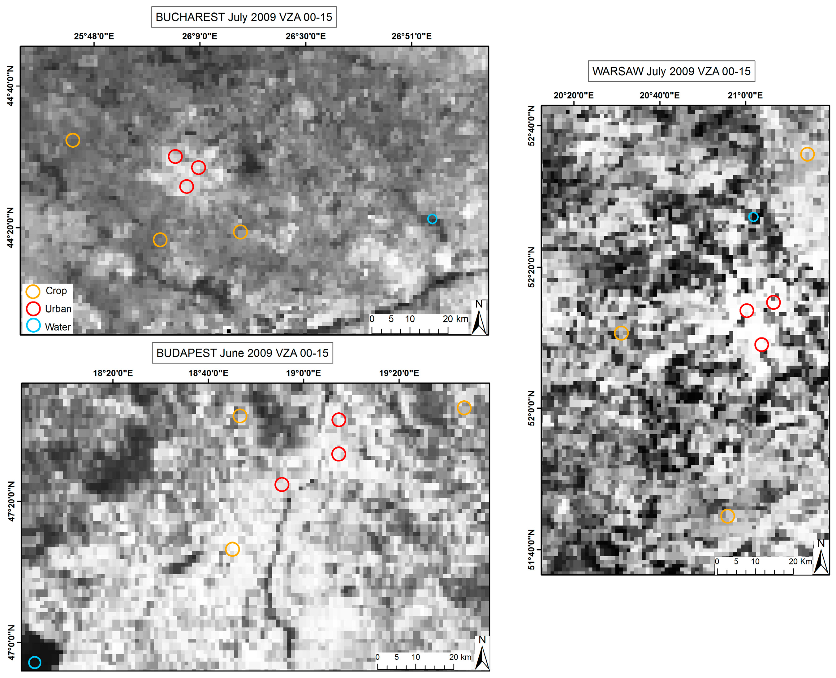
2.1. Study Area

The three study cities—Warsaw, Budapest, and Bucharest—are located in East-Central Europe (Figure 1). They are similar in population, but the area of Budapest and Warsaw is each more than twice the area of Bucharest (

Table 1. Population and area of the three study cities.

City	Population (Millions)		Area (km2)
	2003	2012
Bucharest	1.90	1.88	238
Budapest	1.71	1.72	525
Warsaw	1.68	1.71	517

).

The key similarity between these three capital cities is the shared legacy of centralized planning in which the state had a near-monopoly on urban development until 1990. As a result, their spatial characteristics are sufficiently different from those in Western European cities of comparable size [24]. The original type of spatial structure is characterized by a dense and more compact city center with an abundance of governmental buildings, with the massive size of the socialist pre-fabricated estates and panel-made residential areas [25]. Now, “post-socialist” cities are mostly from the west side of the former Iron Curtain, however, they remain similar to each other.

According to the Köppen–Geiger climate classification, Bucharest has a humid subtropical climate (Cfa), Budapest has an oceanic climate (Cfb), and Warsaw has a warm, humid continental climate (Dfb) [30].

We selected samples of five land cover classes in and around each city, based on the International Geosphere–Biosphere Programme (IGBP) land cover scheme from the MODIS land cover product (MCD12Q1): croplands, forest, mixed croplands-natural vegetation, urban/impervious surface, and open water. We focused on three strongly contrasting classes: croplands, urban, and open water.

2.2. Data Sets

We used Level 1B calibrated radiance data from band 23 (4.020–4.080 μm) of the AQUA MODIS sensor at ascending passes during 2003–2012, with a nominal spatial resolution of 1 km, and near-daily temporal resolution. The MYD021KM product data were downloaded from Level 1 and Atmosphere Archive and Distribution System (LAADS) website (http://ladsweb.nascom.nasa.gov/) as post-processed images that included reprojection into the Universal Transverse Mercator (UTM) coordinate system.

We acquired vegetation product (MYD13A2) of the AQUA MODIS sensor from the LAADS website. Data are provided every 16 days as a composite of maximum value at 1 km spatial resolution. We used the Normalized Difference Vegetation Index (NDVI) from April to October (vegetation season) from 2003 to 2012. The data processing steps were equivalent to those used for MIR data to facilitate comparisons.

We acquired weather data—average monthly air temperature (°C), and average monthly total precipitation (mm)—for each year from the World Weather Website (http://www.tutiempo.net/en), and from the NOAA National Centers for Environmental Information (NCEI) (http://www.ncdc.noaa.gov).

2.3. Methods

Data for each city were processed into one of four different time series depending on the viewing geometry: VZA classes of 0°–15°, 15°–30°, 30°–45°, and 45°–60°. For each year, daily images were sorted by VZA class and stacked and processed into a monthly image based on the maximum MIR values to attenuate effects of cloud cover. Composites from the winter period (October to March) were often affected by compositing artifacts such as dark or bright stripes in either horizontal or vertical orientation.

In each city, we selected quasi-homogeneous areas, each comprising ~9 km² (usually 3 × 3 pixels, but water samples’ shapes varied) for each of the three cover classes. To select our test sites, we used the International Geosphere–Biosphere Programme (IGBP) land cover scheme (Type 1) which provided the same definition of classes for all the three cities. We used class number 13: (urban and built-up) for urban class and 12 (croplands) for agriculture class. While the area of cities is not equal, we used MODIS land cover product (MCD12Q1) with a higher spatial resolution of 500 m to reduce uncertainty. The samples, each for urban and cropland classes, were averaged, but only a single dark open water sample was selected in each scene.

We averaged samples by the city, by VZA, by cover class, and by month for each year, as well as for the decade to characterize the seasonal behavior of MIR radiance. These averaged samples were used for the comparisons among the three east central European capital cities. The NDVI data were processed the same way as MIR. We used the same locations as MIR samples and averaged them in a similar manner.

We compared MIR radiance in cover classes between cities and the simple difference in MIR radiance between urban and croplands. We also used the water sample in each city to normalize the simple difference (urban MIR-cropland MIR)/water MIR). MIR radiance from open water was relatively stable with a lower dynamic range radiance [31], although changes in the temperature of the water body will affect MIR radiance slightly. We analyzed MIR radiance by class as a function of VZA, and we compared the seasonal pattern of MIR radiance with the NDVI. According to the previous studies [23], results show promise in usage for the discrimination of different vegetation types, the estimation of total and leaf biomass of forest ecosystems, and—most important in the light of our study—monitoring intra- and inter-annual changes in vegetation. These results also show that MIR reflectance has been more useful than the NDVI for areas with very high and dense biomass because of larger spectral contrast compared to visible and near-infrared wavelengths, and/or high aerosol loads in the atmosphere [22]. So, MIR was successfully incorporated into vegetation index VI3 (NIR–MIR/NIR + MIR) where it was used instead of red wavelength, as in the NDVI, where atmospheric attenuation effects are reduced [31]. Furthermore, the reflected component of MIR radiation from a vegetation canopy is a function of the liquid water content of the canopy, and water content within leaves is usually less variable than chlorophyll content [32] which makes MIR more stable. Additionally, studies comparing the NDVI response and canopy water amount for forest environments have noted a limited range in NDVI compared with canopy water amount [32]. This reasoning encouraged us to examine the MIR and NDVI response especially in the context of seasonality and distinguishability of different land cover classes.

We explore the influence of latitude on MIR seasonality through the lens of the convex quadratic model as follows:

MIR_m = α + β × AMMIR − γ × AMMIR²

(1)

where MIR_m is the monthly value of MIR radiance, AMMIR is the accumulated monthly MIR radiance, and α, β, and γ are parameter coefficients. From the fitted coefficients, two metrics can be calculated to summarize the model:

Peak_MIR = α − (β²/4 × γ)

(2)

TTP_MIR = −β/2 × γ

(3)

where Peak_MIR is the peak value of MIR in the fitted model, and TTP_MIR is the time to peak, i.e., the accumulated MIR radiance at the point of the peak value of MIR in the fitted model.

This model relates monthly MIR radiance with accumulated monthly MIR radiance. Two shape metrics of the model—time to peak (in terms of accumulated radiance) and peak height (in terms of radiance amplitude)—aid comparisons across cover classes and cities.

Finally, we explored the influence of meteorological variables—accumulated monthly precipitation and maximum monthly air temperature—on MIR seasonality to identify some simple associations between weather and observed MIR radiance.

3. Results

3.1. Multiannual Analyses

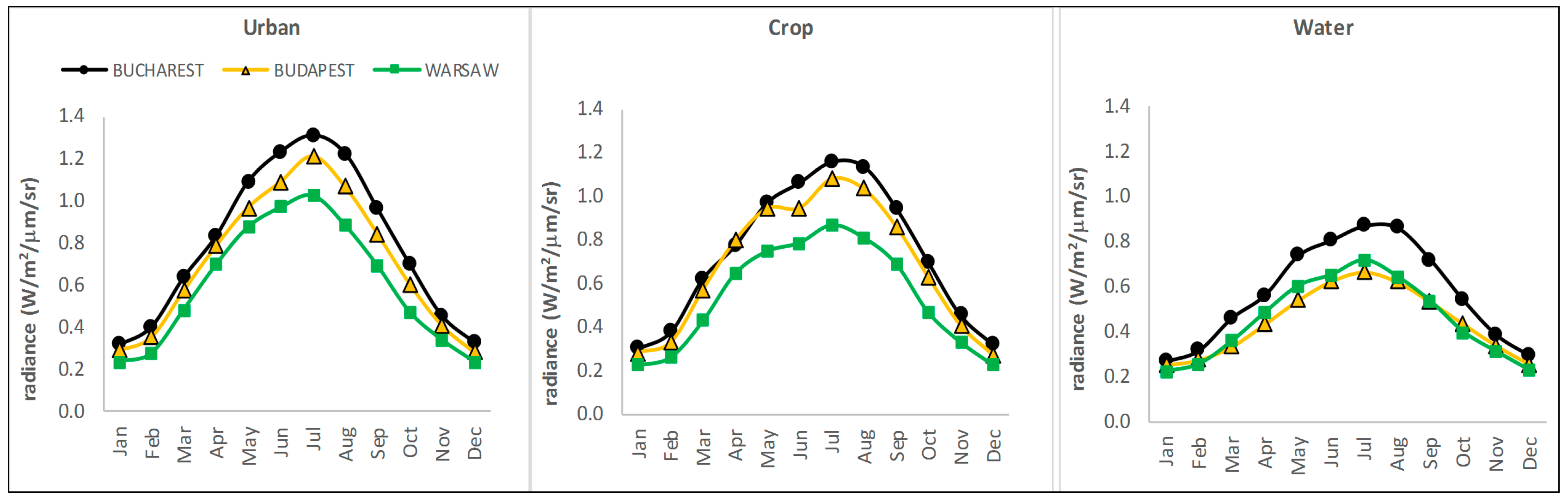
3.1.1. Multiannual Average Comparison and Water Normalization

The first step was to explore the pattern of MIR response by calculating multiannual monthly values. The seasonal pattern of MIR radiance is similar across the three cities. The unimodal seasonality peaks in July and is lowest during the winter months, with values for Warsaw that are consistently lower than Bucharest and Budapest, in between for urban and cropland and sometimes lower than Warsaw for the open water samples (Figure 2). As the year progresses, the differences between the cities increase and peak in mid-summer. Urban trajectories are almost symmetrical in contrast to croplands, which show a two-phase pattern that includes a pause or slowing of the increase of MIR radiance in June. The difference between maximum radiance of urban and cropland classes is about 0.15 W/m²/µm/sr. The dynamic ranges of water samples are more muted but show distinct seasonality (Figure 2).

The simple difference and normalized difference data show similar seasonal patterns, but the normalization helps to underscore the differences in MIR radiance between urban and cropland covers (Figure 3). Differences are lowest in Bucharest and highest in Warsaw. In early spring (March) and autumn (September and October), the differences between Bucharest and Budapest are negligible but positive in Warsaw, suggesting that snow cover might be attenuating MIR radiance in Poland. In Budapest, negative values occurred both in April and during autumn. Negative values indicate higher MIR radiance from cropland than urban cover, which is to be expected from large expanses of MIR-bright bare soils that occur at planting and again at harvest.

3.1.2. NDVI Comparison

Vegetation cover is common in urban areas. Green vegetation appears bright in the near infrared in contrast to its dark appearance in the MIR [20]. The normalized difference vegetation index (NDVI) is calculated based on the difference between near-infrared and red reflectances normalized by their sum [33]; thus, the NDVI has higher values when a pixel has a larger fraction of green vegetation cover. Thus, for urban impervious surfaces and bare soils the NDVI is low. To compare the “greenness” of the urban–rural groupings and their seasonality relative to the seasonality of MIR radiance, we first extracted the average April to October NDVI patterns from the urban and cropland sites for each city (Figure 4).

Budapest and Warsaw exhibit almost similar values for the whole season (the maximum values are 0.48 and 0.49, respectively). In Bucharest, the maximum value is equal to 0.37, which is comparable to the growing seasonal minimum value of other cities. This low NDVI likely results from fewer green space areas within Bucharest compared to other cities [34,35]. Additionally, the relative change of the NDVI during the season is limited (0.08, 0.09, 0.12 for Bucharest, Budapest, and Warsaw, respectively). A different situation was found for cropland areas. Peaks occurred early (May for southerly Bucharest and June for Budapest and Warsaw) with gradual declines as the season progressed. The seasonal amplitude was found in Budapest (0.26), then for Bucharest (0.18) and Warsaw (0.16). Both latitudinal effects on climate and regional crop differences likely explain these differences in timing and amplitude.

Does MIR radiance inversely mirror NDVI seasonality (Figure 5)? The MIR shows a larger dynamic range between land covers than the NDVI: ~0.30 vs. ~0.15. The changes in the normalized MIR radiances are rapid relative to the NDVI, particularly in the early growing season: the pace of divergence between city and cropland are faster in the MIR than the NDVI. An interesting feature occurs in October in Budapest where MIR radiance of croplands is greater than the city, and the NDVI of the city is larger than the croplands (Figure 6).

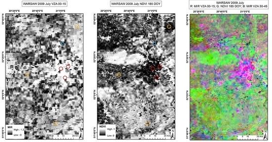
3.1.3. View Zenith Angle Effects

The MYD021KM product includes the view zenith angle (VZA) for each acquisition. Evaluating MIR radiance by VZA is important because the MIR signal is low [21,22]. Early in the year, every VZA class increases in a similar manner but divergence starts in April after the vernal equinox, and peaks in July after the summer solstice (Figure 7 and Figure 8).

A higher dynamic range in MIR radiance in all VZA classes occurs in Bucharest than Warsaw. In Warsaw, the off-nadir sequences (higher VZAs) show the lower dynamic range and smoother transitions for both urban (Figure 7) and cropland (Figure 8) samples.

The temporal variation in MIR radiance is more pronounced in the croplands with an evident bimodality, particularly in Budapest (Figure 8). The influence on MIR response is a result of the bare soil surface detection, which is pronounced by bimodality during summer season (especially in Budapest).

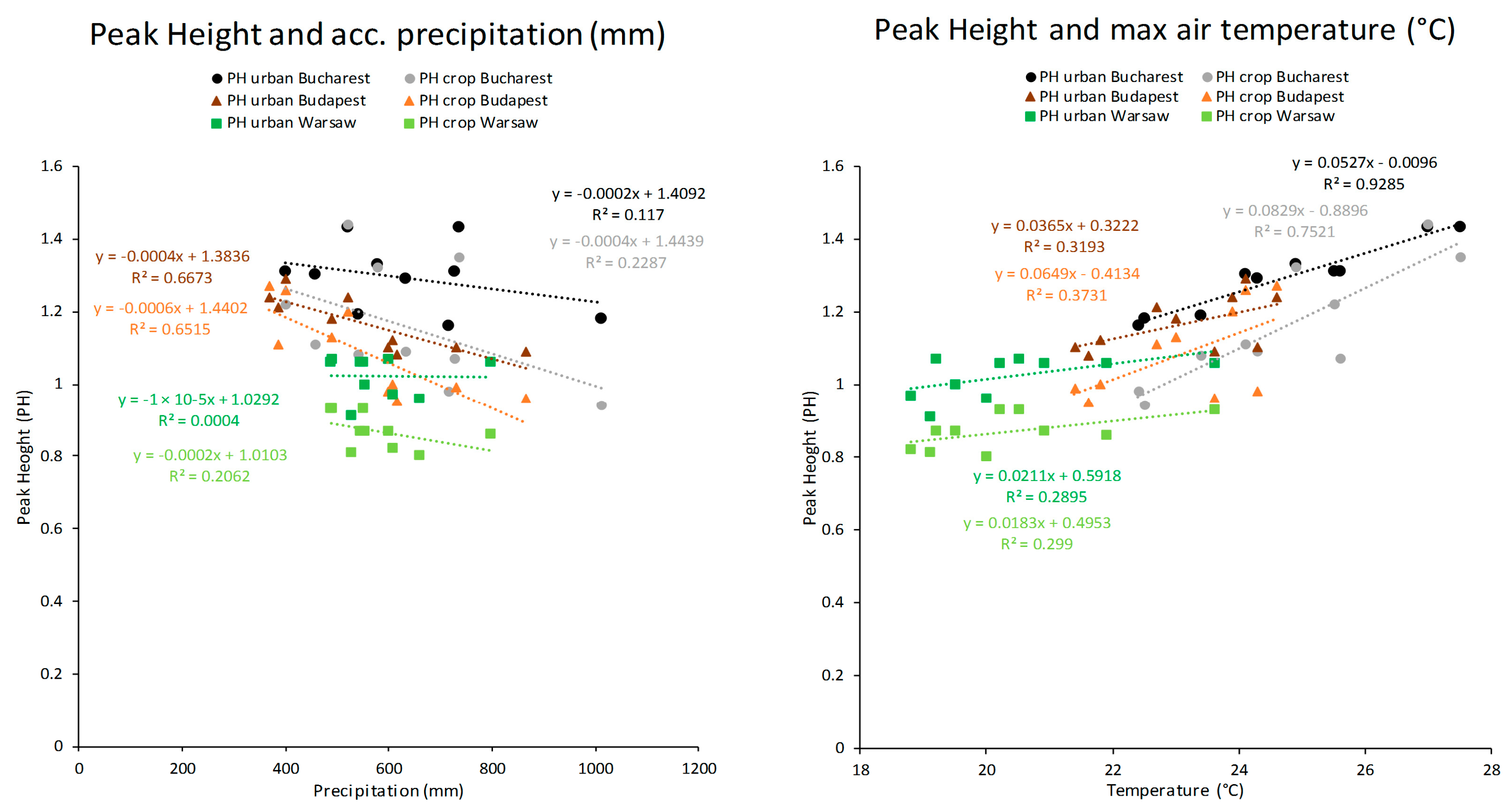
3.1.4. Accumulated Radiance and the Convex Quadratic (CxQ) Model

As the final step in the analysis of multiyear averages, we fitted a CxQ model of the monthly MIR radiance as a function of accumulated monthly MIR radiance (Figure 9). The quadratic model reveals how much the accumulated MIR radiance varies by latitude: greatest in Bucharest at 44.4° N and least in Warsaw at 52.2° N (

Table 2. Metrics characterizing the fitted curves of Figure 9: modeled annual peak MIR radiance (Peak Height: PH) and accumulated monthly MIR radiance at annual peak (Time to Peak: TTP).

	Urban		Crop		Urban-Crop
	TTP	PH	TTP	PH	TTP	PH
Bucharest	5.07	1.29	4.76	1.16	0.31	0.13
Budapest	4.53	1.17	4.37	1.08	0.16	0.09
Warsaw	3.73	1.02	3.41	0.87	0.32	0.15

).

For all cities in urban class, a very strong (r² higher than 0.97) parabolic pattern is visible. The highest accumulated monthly MIR (Table 2) is in Bucharest (5.07 W·m⁻²) with the peak of 1.29 (W·m⁻²). The lowest values of TTP and PH are in Warsaw. Within the cropland class; the pattern has r² higher than 0.95. While the difference of TTP and PH between Bucharest and Warsaw is the same apart from the land cover class (TTP: 1.34 and 1.36, PH: 0.27 and 0.29 for urban and cropland respectively), then the difference between Budapest and Warsaw increased (TTP: 0.80 and 0.97, PH: 0.14 and 0.21). Consequently, the difference between Bucharest and Budapest decreased (TTP: 0.54 and 0.39, PH: 0.13 and 0.08).

The difference in TTP and PH between urban and crop is the biggest for Warsaw, then for Bucharest. Budapest expresses the lowest difference.

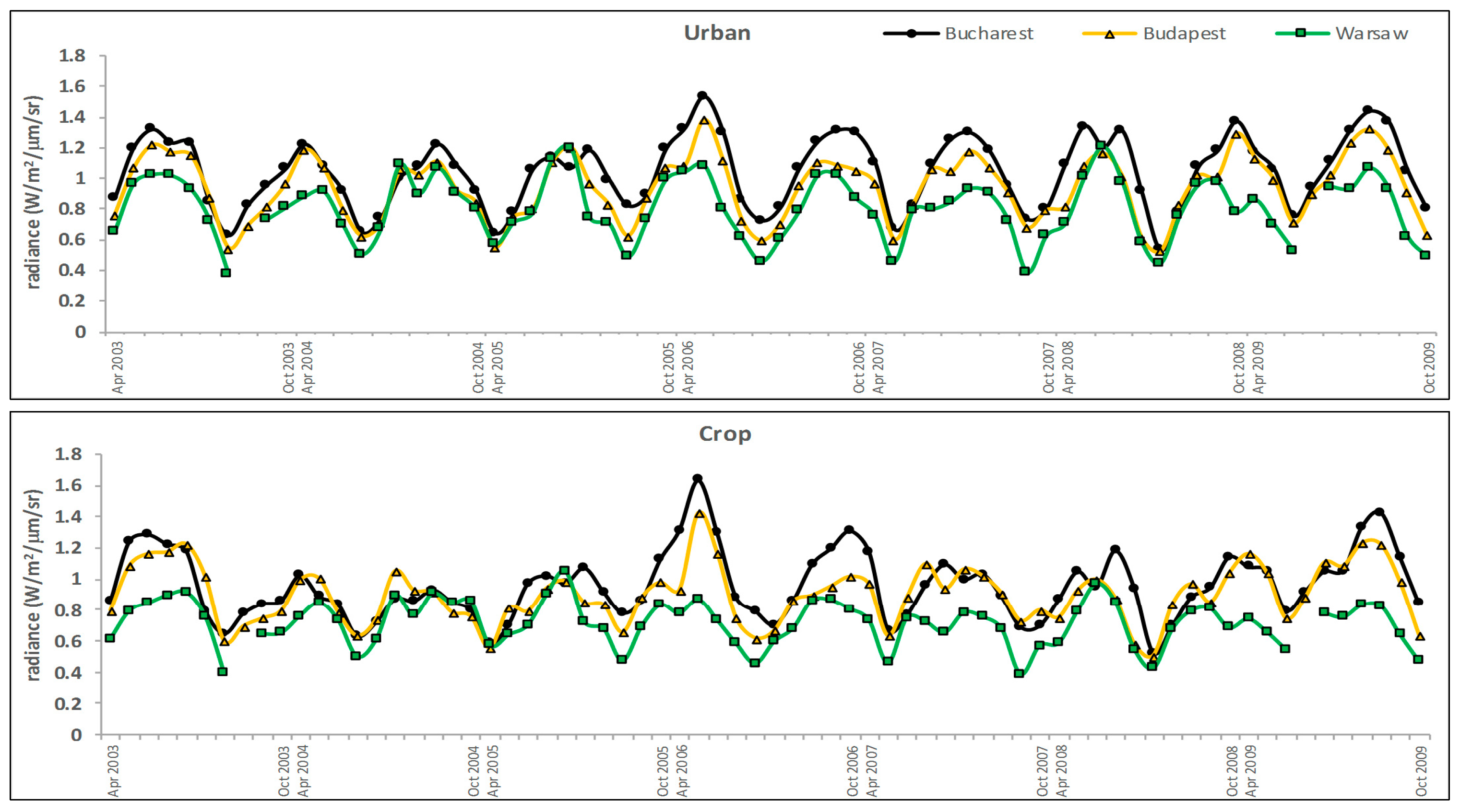
3.2. Time Series Analyses over Years 2003–2012 from April to October

In the second part of this study, we focused on seasonal MIR behavior over 2003–2012 from April to October (Figure 10). We investigated time series data of MIR using additional information about monthly mean temperature and accumulated mean monthly precipitation for each year (Figure 11). Generally, as seen above, the MIR radiance is greatest in Bucharest and the lowest in Warsaw. However, in some years, the weather impact was strong enough to change this pattern [28,29]. The MIR radiation, as explained in the introductory part, is a mix of reflected and emitted radiation. Our contemplation about weather impact is connected with the insolation and ground warming. Precipitation cools the ground and affects the emittance; additionally, cloudiness increases. However, the indirect influence on reflectance can be a result of a higher groundwater lever (higher moisture—darker color—lower spectral response) which results in better vegetation health. The more dense the vegetation, the lower is the MIR radiance. Drier conditions can lead to sparser vegetation, a shortened growing season, and higher MIR brightness due to more exposed soil. The timing of weather events is also important. For example, intense precipitation occurring after the maximum MIR radiance, such as in autumn, may generate a rapid decrease in MIR radiance but have no effect on the composited maximum MIR value.

3.2.1. Bucharest

In 2007, the annual maximum MIR radiance was highest (

Table 3. The maximum values of MIR radiance from each year for urban and cropland class for three cities. Red indicates the highest value and blue indicates the lowest value in the time series.

	Max MIR	2003	2004	2005	2006	2007	2008	2009	2010	2011	2012	MEAN
Bucharest	Urban	1.32	1.22	1.22	1.18	1.53	1.32	1.30	1.34	1.37	1.44	1.33
	Crop	1.29	1.03	0.93	1.08	1.64	1.31	1.10	1.19	1.15	1.43	1.21
Budapest		1.22	1.19	1.11	1.20	1.39	1.10	1.18	1.17	1.30	1.32	1.22
		1.23	1.01	1.05	0.99	1.43	1.02	1.10	1.00	1.17	1.23	1.12
Warsaw		1.03	0.92	1.09	1.20	1.09	1.02	0.94	1.21	0.98	1.07	1.05
		0.92	0.85	0.91	1.05	0.87	0.87	0.79	0.98	0.81	0.84	0.89

) for both urban (1.53) and cropland (1.64) classes. There was a notable heat wave in southeastern Europe in 2007, with the average monthly maximum temperature reaching 27 °C (

Table 4. Accumulated annual precipitation (mm) and maximum air temperature for each city (°C). Red color indicates the maximum value and blue color the minimum value in the annual time series.

	Weather	2003	2004	2005	2006	2007	2008	2009	2010	2011	2012	MEAN
Bucharest	(mm)	578.6	716.8	1013.4	541.2	520.9	400.3	632.6	728.0	459.2	736.9	632.79
	(°C)	24.9	22.4	22.5	23.4	27.0	25.5	24.3	25.6	24.1	27.5	24.72
Budapest		369.0	616.2	732	597.9	522.8	608.6	488.7	867.1	387.6	400.6	559.05
		24.6	21.6	21.4	24.3	23.9	21.8	23.0	23.6	22.7	24.1	23.10
Warsaw		550.9	527.0	490.5	488.1	599.9	552.9	659.2	796.5	608.7	544.1	581.78
		20.2	19.1	20.5	23.6	19.2	19.5	20.0	21.9	18.8	20.9	20.37

). The precipitation in 2007 was very low (520.9 mm) and even lower the following year (400.3 mm). The lowest max MIR (1.18) for the urban class was in 2006 (in July). We explain it by the fact that in the images for three VZA classes—0°–15°, 15°–30°and 30°–45°—the pixels from urban and cropland samples had no values because of a compositing artifact. So, considering the second lowest max MIR radiance for urban which happened in years 2004 and 2005 (1.22), we see that these two years were very wet by high precipitation and the lowest maximum air temperature (lower than mean air temperature from 2003 to 2012). The lowest maximum MIR radiance in cropland occurred in 2005 (0.93) when the accumulated precipitation was the highest (1013.4 mm). Higher precipitation may increase vegetation cover, thereby darkening the surface in the MIR.

3.2.2. Budapest

Similar to Bucharest, the highest maximum MIR radiances occurred in 2007 with 1.39 for urban and 1.43 for cropland (Table 3). During 2007, accumulated precipitation was below the mean from 2003 to 2012 and the maximum air temperature was higher (Table 4). The 2003 European heatwave [36] impacted Budapest with the highest maximum air temperature and the lowest accumulated precipitation (Table 4). However, the MIR radiance from the urban areas equaled the multiyear average; in contrast, the cropland’s maximum MIR radiance was 10% greater than the average, lower than 2007.

3.2.3. Warsaw

The extreme heat occurred in Poland in 2006: maximum air temperature was greatest, and precipitation was least (Table 4). In 2006 the maximum urban MIR radiance was the second highest, and the cropland MIR radiance was the highest (Table 3). Curiously, it was very wet in Warsaw and Budapest in 2010 (although the heat and drought in European Russia were extreme [37]); yet, maximum urban MIR radiance was greatest the same year. The lowest maximum MIR radiance for urban occurred in 2004 and in 2009 for cropland (Table 3).

Finally, we examined the relationships between the two fitted CxQ model metrics for 2003–2012 years and weather conditions. Figure 12 shows the relationship between TTP and accumulated precipitation (Figure 12left) and maximum air temperature (Figure 12right). The TTPs for urban and cropland exhibit negative correlations with accumulated precipitation, but the strength of the relationships is strong in Budapest, marginal in Bucharest, and very weak in Warsaw. The TTPs show strong positive correlations with maximum air temperature in Bucharest, but not in either Budapest or Warsaw. Peak heights for urban and cropland in Budapest are negatively correlated with accumulated precipitation (Figure 13left). While there is a strong positive correlation between maximum air temperature and peak heights for Bucharest, the positive relationships for Budapest and Warsaw are modest (Figure 13right).

4. Discussion

The urban heat island effect results not just from emittance in the longer wavelengths of the thermal infrared, but also from the emittance in the shorter wavelengths of the middle infrared. During the daytime, there is also a minor contribution from reflected sunlight. The 4 μm wavelengths from band 23 of MODIS has the advantage of penetrating urban haze and smoke and, thus, may be able to provide more consistent views of the urbanizing land surface, particularly in the tropics where the aerosol optical depth over cities is frequently very high. We do not, however, quantify the influence of the MIR on sensible heat. Instead, we have illustrated here how MIR time series can reveal the urban radiation anomaly at wavelengths shorter than TIR and how this effect has a distinct seasonality that arises from multiple factors.

First, latitudinal variation affects the radiation anomaly in MIR due to the weaker insolation at higher latitudes. A second and related factor is the climate zone. Warsaw is exposed to air masses from the Baltic Sea and therefore has a more humid climate than in Budapest. Bucharest is located in a different climate zone in warmer southeastern Europe. Third, the contrast between urban and cropland in the MIR is not constant due to changes in the amount and timing of exposed soils due to crop types and agricultural practices. Urban MIR seasonality is unimodal with peak radiance shortly after the summer solstice. In contrast, cropland seasonality can be slightly bimodal as the process of planting exposes MIR-bright soils, and then the surface darkens in the MIR due to crop growth covering the soil surface, and then brightens again due to the drying of the vegetation prior to harvest. Fourth, both temperature and precipitation modulate MIR seasonality, but not in a simple way. Temperature may provide a proxy of insolation and dryness, driving the land surface to a brighter MIR state. Precipitation may be driving the land surface to a darker MIR state through stimulating vegetation growth and development. However, the sequence of weather—the mixture of sun and rain—can force the vegetated land surface in various directions, some MIR brightening, and some MIR darkening. Thus, the MIR data provide a complement to other remote sensing approaches to the characterization of urban structure and function.

Using open water to normalize the differences between urban and cropland MIR radiance helped to emphasize the contrasts. Yet, not all areas have sufficiently large bodies of open water nearby, and the depth of the lake or reservoir should affect how MIR-dark the surface is and, thus, affect the strength of the normalization. A shallower or smaller lake may heat more quickly than a large body; thus, comparisons of normalized differences must be done with caution [24]. However, it appears as a simple first approximation to facilitate comparisons in the MIR. It is clear that the phenomenology of the MIR is not a simple inverse of the NDVI, but rather responds to surface conditions and environmental forcing in a manner that is complementary to vegetation indices [20]. Likewise, the use of the accumulated radiance through the CxQ model was able to capture differences among the cities and other cover types.

There are limitations to the broader use of the MIR in urban studies. The coarse spatial resolution (~1 km at nadir) of current orbital sensors with MIR capability makes it difficult to resolve the spatially heterogeneous land cover patterns that exemplify most cities. Although there are airborne sensors with finer spatial resolution in the MIR [22], we do not expect a new satellite system in the foreseeable future with higher MIR resolution. The European Space Agency’s environmental satellite Sentinel 3—Global Sea/Land Monitoring Mission that launched 16 February 2016—has two bands centered at 3.74 μm in the Sea and Land Surface Temperature Radiometer (SLSTR) for the measurement of skin temperature and the detection of active fires. While resolving the MIR seasonality of particular buildings or blocks may not be possible at 1 km, there might be potential to compare the MIR behaviors of different elements in the urban fabric using Local Climate Zones [19].

5. Conclusions

We have shown that there exists an urban radiation anomaly in the middle infrared region and that this anomaly has a strong seasonality which results from multiple factors. There are many studies about UHI using land surface temperature derived from thermal infrared data, but there are few studies exploring the benefits and limitations of using MIR for urban science. Cities are complex and changing entities on the land surface that interact across multiple scales with their environment. Within these heterogeneous landscapes, there are many factors which contribute to urban radiation anomalies: type of buildings, density and spatial arrangement, properties of construction and roofing materials, urban geometry or green areas’ size. By viewing the urbanizing surface at wavelengths between the familiar regions of the thermal infrared and the visible to near infrared, we expect new insights, particularly where air pollution may veil the variegated city much of the year. These results on the urban–rural contrasts in three cities in central-eastern Europe pave the way to extending this analysis to burgeoning cities of tropical South Asia.

References

1. Seto, K.C.; Fragkias, M.; Güneralp, B.; Reilly, M.K. A meta-analysis of global urban land expansion. PLoS ONE 2011, 6, 8. [Google Scholar] [CrossRef]
2. Grimm, N.B.; Faeth, S.H.; Golubiewski, N.E.; Redman, C.L.; Wu, J.; Bai, X.; Briggs, J.M. Global change and the ecology of cities. Science 2008, 319, 756–760. [Google Scholar] [CrossRef]
3. Martin, P.; Baudouin, Y.; Gachon, P. An alternative method to characterize the surface urban heat island. Int. J. Biometeorol. 2015, 59, 849–861. [Google Scholar] [CrossRef]
4. Oke, T.R. The energetic basis of the urban heat island. Q. J. R. Meteorol. Soc. 1982, 108, 1–24. [Google Scholar] [CrossRef]
5. Krehbiel, C.P.; Jackson, T.; Henebry, G.M. Web-Enabled Landsat Data time series for monitoring urban heat island impacts on land surface phenology. IEEE J. Sel. Top. Appl. Earth Observ. Remote Sens. 2016, 9, 2043–2050. [Google Scholar] [CrossRef]
6. Krehbiel, C.P.; Henebry, G.M. A comparison of multiple datasets for monitoring thermal time in urban areas over the U.S. Upper Midwest. Remote Sens. 2016, 8, 297. [Google Scholar] [CrossRef]
7. Lemonsu, A.; Viguié, V.; Daniel, M.; Masson, V. Vulnerability to heat waves: Impact of urban expansion scenarios on urban heat island and heat stress in Paris (France). Urban Clim. 2015, 14, 586–605. [Google Scholar] [CrossRef]
8. Arnfield, A.J. Two decades of urban climate research: A review of turbulence, exchanges of energy and water, and the urban heat island. Int. J. Climatol. 2003, 23, 1–26. [Google Scholar] [CrossRef]
9. Hooke, R.L.; Martín-Duque, J.F. Land transformation by humans: A review. GSA Today 2012, 22, 4–10. [Google Scholar] [CrossRef]
10. Tran, H.; Uchihama, D.; Ochi, S.; Yasuoka, Y. Assessment with satellite data of the urban heat island effects in Asia mega cities. Int. J. Appl. Earth Observ. Geoinform. 2006, 8, 34–48. [Google Scholar] [CrossRef]
11. Imhoff, M.L.; Zhang, P.; Wolfe, R.E.; Bounoua, L. Remote sensing of the urban heat island effect across biomes in the continental USA. Remote Sens. Environ. 2010, 144, 504–513. [Google Scholar] [CrossRef]
12. Streutker, D.R. Satellite-measured growth of urban heat island of Houston, Texas. Remote Sens. Environ. 2003, 85, 282–289. [Google Scholar] [CrossRef]
13. Weng, Q. Thermal infrared remote sensing for urban climate and environmental studies: Methods, applications, and trends. ISPRS J. Photogramm. Remote Sens. 2009, 64, 335–344. [Google Scholar] [CrossRef]
14. Voogt, J.A.; Oke, T.R. Thermal remote sensing of urban climates. Remote Sens. Environ. 2003, 86, 370–384. [Google Scholar] [CrossRef]
15. Tomlinson, C.J.; Chapman, L.; Thorne, J.E.; Baker, C. Remote sensing land surface temperature for meteorology and climatology: A review. Meteorol. Appl. 2011, 18, 296–306. [Google Scholar] [CrossRef]
16. Potere, D.; Schneider, A. A critical look at representations of urban areas in global maps. GeoJournal 2007, 69, 55–80. [Google Scholar] [CrossRef]
17. Gallo, K.P.; McNab, A.L.; Karl, T.R.; Brown, J.F.; Hood, J.J.; Tarpley, J.D. The use of NOAA AVHRR data for assessment of the urban heat island effect. J. Appl. Meteorol. 1993, 32, 899–908. [Google Scholar] [CrossRef]
18. Stewart, I.D.; Oke, T.R. Local climate zones for urban temperature studies. Bull. Am. Meteorol. Soc. 2012, 93, 1879–1900. [Google Scholar] [CrossRef]
19. Ju, J.; Roy, D.P. The availability of cloud-free Landsat ETM+ data over the conterminous United States and globally. Remote Sens. Environ. 2008, 112, 1196–1211. [Google Scholar] [CrossRef]
20. Henebry, G.M. Mapping Human Settlements Using the mid-IR: Advantages, Prospects, and Limitations, in Urban Remote Sensing; Weng, Q., Quattrochi, D., Eds.; CRC Press: Boca Raton, FL, USA, 2007; pp. 339–355. [Google Scholar]
21. Krehbiel, C.P.; Kovalskyy, V.; Henebry, G.M. Exploring the middle infrared region for urban remote sensing: Seasonal and view angle effects. Remote Sens. Lett. 2013, 4, 1147–1155. [Google Scholar] [CrossRef]
22. Boyd, D.S.; Petitcolin, F. Remote sensing of the terrestrial environment using middle infrared radiation (3.0–5.0 μm). Int. J. Remote Sens. 2004, 25, 3343–3368. [Google Scholar] [CrossRef]
23. Tomaszewska, M.; Kovalskyy, V.; Small, C.; Henebry, G.M. Viewing global megacities through MODIS radiance: Effects of time of year, latitude, land cover, and view zenith angle. IEEE J. Sel. Top. Appl. Earth Observ. Remote Sens. 2016, 9, 3753–3760. [Google Scholar] [CrossRef]
24. Ianoş, I.; Sîrodoev, I.; Pascariu, G.; Henebry, G.M. Divergent patterns of built-up urban space growth following post-socialist changes. Urban Stud. 2015. [Google Scholar] [CrossRef]
25. Hirt, S. Whatever happened to the (post) socialist city? Cities 2013, 32 (Suppl. 1), S29–S38. [Google Scholar] [CrossRef]
26. Henebry, G.M.; de Beurs, K.M. Remote sensing of land surface phenology: A prospectus. In Phenology: An Integrative Environmental Science; Schwartz, M.D., Ed.; Springer: New York, NY, USA, 2013; pp. 385–411. [Google Scholar]
27. De Beurs, K.M.; Henebry, G.M. Land surface phenology and temperature variation in the IGBP high-latitude transects. Glob. Chang. Biol. 2005, 11, 779–790. [Google Scholar] [CrossRef]
28. Coumou, D.; Robinson, A.; Rahmstorf, S. Global increase in record-breaking monthly-mean temperatures. Clim. Chang. 2013, 118, 771–782. [Google Scholar] [CrossRef]
29. Meehl, G.A.; Tebaldi, C. More intense, more frequent and longer lasting heat waves in the 21st century. Science 2004, 305, 994–997. [Google Scholar] [CrossRef]
30. Kottek, M.; Grieser, J.; Beck, C.; Rudolf, B.; Rubel, F. World Map of the Köppen-Geiger climate classification updated. Meteorol. Z. 2006, 15, 259–263. [Google Scholar] [CrossRef]
31. Cracknell, A.; Boyd, D.S. Interactions of Middle Infrared (3–5 µm) Radiation with the Environment. In The Sage Handbook of Remote Sensing; Warner, T.A., Nellis, M.D., Foody, G.M., Eds.; Sage: Thousand Oaks, CA, USA, 2009. [Google Scholar]
32. Boyd, D.S.; Wicks, T.E.; Curran, P.J. Use of middle infrared radiation to estimate the leaf area index of a boreal forest. Tree Physiol. 2000, 20, 755–760. [Google Scholar] [CrossRef]
33. Tucker, C.J. Red and photographic infrared linear combinations for monitoring vegetation. Remote Sens. Environ. 1979, 8, 127–150. [Google Scholar] [CrossRef]
34. Fuller, R.A.; Gaston, K.J. The scaling of green space coverage in European cities. Biol. Lett. 2009, 5, 352–355. [Google Scholar] [CrossRef]
35. Petrişor, A. Assessment of the green infrastructure of Bucharest using Corine and Urban Atlas data. Urban. Archit. Constr. 2015, 6, 19–24. [Google Scholar]
36. García-Herrera, R.; Diaz, J.; Trigo, R.M.; Luterbacher, J.; Fischer, E.M. A review of the European summer heat wave of 2003. Crit. Rev. Environ. Sci. Technol. 2010, 40, 267–306. [Google Scholar] [CrossRef]
37. Wright, C.K.; de Beurs, K.M.; Henebry, G.M. Land surface anomalies preceding the 2010 Russian heat wave and a link to the North Atlantic Oscillation. Environ. Res. Lett. 2014, 9, 124015. [Google Scholar] [CrossRef]
Figure 1. Image of Bucharest (top), Budapest (bottom), Warsaw (right) with samples of land cover classes: orange—croplands, red—urban, blue—water. Images are the July 2009 middle infrared radiance at a View Zenith Angle (VZA) class of 0°–15°.
Remotesensing 08 00924 g001
Figure 2. Mean monthly MIR radiance across cities for three classes: urban, cropland, and water.
Remotesensing 08 00924 g002
Figure 3. Differences between land cover classes: urban and cropland of multiannual monthly mean values of MIR radiance for all cities (left) and these differences normalized by MIR radiance from open water class (right).
Remotesensing 08 00924 g003
Figure 4. Average normalized difference vegetation index (NDVI) for urban (left) and cropland (right) classes for the three study cities.
Remotesensing 08 00924 g004
Figure 5. Image of Warsaw with samples of land cover classes: orange—croplands, red—urban, blue—water. Images are: July 2009 MIR composite at a view zenith angle (VZA) class of 0°–15° (left); NDVI July 2009 (middle); and False color composite for July 2009 R: MIR VZA 0°–15°, G: NDVI, B: MIR VZA 30°–45° (right).
Remotesensing 08 00924 g005
Figure 6. Simple differences in mean MIR radiance between urban and cropland classes (left); Normalized differences in mean MIR radiance between urban and cropland classes (middle); Simple differences in mean NDVI between urban and cropland classes (right).
Remotesensing 08 00924 g006
Figure 7. Mean monthly values of MIR radiance in four VZA classes for the urban cover class.
Remotesensing 08 00924 g007
Figure 8. Mean monthly values of MIR radiance in four VZA classes for the cropland class.
Remotesensing 08 00924 g008
Figure 9. Fitted Convex Quadratic (CxQ) models for urban (left) and cropland (right) classes for each city.
Remotesensing 08 00924 g009
Figure 10. Time series chart of MIR radiance for urban (top) and cropland (bottom) classes from April to October over 2003–2012.
Remotesensing 08 00924 g010
Figure 11. Weather conditions in Bucharest, Budapest, and Warsaw. Red color indicates monthly mean air temperature (°C) and blue color indicates accumulated monthly precipitation (mm). Dots represent months.
Remotesensing 08 00924 g011
Figure 12. Relationships between time to peak and accumulated precipitation (left) and maximum air temperature (right).
Remotesensing 08 00924 g012
Figure 13. Relationships between peak height and accumulated precipitation (left) and maximum air temperature (right).
Remotesensing 08 00924 g013