An Optimal Sample Data Usage Strategy to Minimize Overfitting and Underfitting Effects in Regression Tree Models Based on Remotely-Sensed Data

Abstract

Regression tree models have been widely used for remote sensing-based ecosystem mapping. Improper use of the sample data (model training and testing data) may cause overfitting and underfitting effects in the model. The goal of this study is to develop an optimal sampling data usage strategy for any dataset and identify an appropriate number of rules in the regression tree model that will improve its accuracy and robustness. Landsat 8 data and Moderate-Resolution Imaging Spectroradiometer-scaled Normalized Difference Vegetation Index (NDVI) were used to develop regression tree models. A Python procedure was designed to generate random replications of model parameter options across a range of model development data sizes and rule number constraints. The mean absolute difference (MAD) between the predicted and actual NDVI (scaled NDVI, value from 0–200) and its variability across the different randomized replications were calculated to assess the accuracy and stability of the models. In our case study, a six-rule regression tree model developed from 80% of the sample data had the lowest MAD (MAD_training = 2.5 and MAD_testing = 2.4), which was suggested as the optimal model. This study demonstrates how the training data and rule number selections impact model accuracy and provides important guidance for future remote-sensing-based ecosystem modeling.

1. Introduction

Satellite remote sensing has become an important tool for land surface and terrestrial ecosystem monitoring [1,2,3,4,5,6,7,8,9,10,11,12]. The main advantages of satellite remote sensing observations include (1) wide and continuous spatial coverages that allow regional to global studies; and (2) high spatial and temporal resolutions that can capture rapid land surface changes (e.g., wildland fire) and seasonal dynamics at fine scales [5,13,14,15,16,17,18,19].

Data-driven regression tree models based on satellite observations, climate and environmental variables, and ground truth data have been successfully used for regional and global land cover mapping and ecosystem modeling [6,20,21,22,23,24,25,26]. The data-driven regression tree approach divides the multi-dimensional data domain of environmental variables into many segments and derives one (or multiple) regression equation(s) for each segment. Results from these previous studies help better understand the regional land surface changes and trends, ecosystem services, and climate change impacts on land surface dynamics.

Cubist software [27], a common tool for predicting continuous ecosystem attributes, develops a generalized set of rules with associated multiple regression models (a series of piecewise regressions) which are constrained by the training data [28,29,30,31]. Generally, a simple sample data usage strategy (e.g., 90% of the sample data for model training and 10% of the sample data for testing the reliability of the model) is applied in the Cubist regression tree model development [4]. However, improper use of the sample data (percentage of the data used for model training and testing) can cause overfitting or underfitting effects [32] and may lead to a bias evaluation of the derived regression tree models [33,34]. Therefore, an approach that seeks to identify optimal model parameters for a dataset (e.g., training and testing sample size, number of rules) is often needed.

The main objective of this study is to develop a method that identifies an optimal sample data usage strategy and rule numbers that minimize over- and underfitting effects and maximize prediction accuracy on unseen data in regression tree mapping models. Regression tree models were developed using nine randomized replications at each training data size from 10% to 90% of the sample data, in 10% increments, using GNU General Public License (GPL) Cubist (version 2.07 GPL Edition) and Python scripts. Accuracy assessments (i.e., training and testing error magnitudes and variation across a wide range of training data sizes) for the derived regression tree models were quantified. Results from this study reveal trends of prediction error and provide an approach for optimizing the accuracy of a Cubist regression tree model [35], which will likely be useful for future remote-sensing-based ecosystem parameter mapping and modeling studies.

2. Materials and Methods

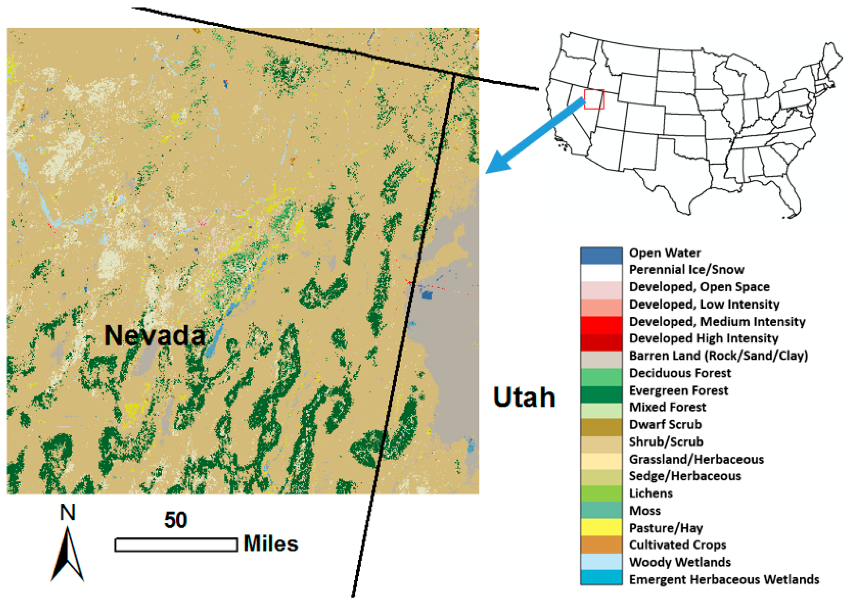
2.1. Case Study Area

A pilot study area located mainly in Northeastern Nevada (Figure 1) was selected for testing. Based on the 2011 National Land Cover Database (NLCD 2011), the main land cover types for the study area are shrub/scrub (75.4%) and forest (10.2%). Other land cover types include barren land (6.6%), herbaceous (4.9%), and hay/pasture (1.2%) [5]. The broad range of land cover types and vegetation biomass productivity in the study area helped to ensure the robustness of the testing results.

2.2. Data Used for Developing and Evaluating Regression Tree Models

2.2.1. Background

The satellite-derived Normalized Difference Vegetation Index (NDVI) is the normalized reflectance difference between the near infrared (NIR) and visible red bands [36,37]. NDVI represents the vigor and photosynthetic capacity (or greenness) of the vegetation canopy [37,38]. The time series of Moderate Resolution Imaging Spectroradiometer (MODIS) NDVI data have been widely used for vegetation dynamic (e.g., land surface phenology) [39] and ecosystem monitoring (e.g., biomass productivity mapping) [40]. The advantages of MODIS data include (1) high temporal resolution (one- to two-day revisit time), which can capture the rapid land changes during the growing season, and (2) a wide range of wavelengths that make the MODIS land surface products robust and reliable (e.g., atmospherically corrected for cloud, cloud shadows, and aerosols) [41]. However, the 250 m MODIS productivity map can only provide coarse-scale pattern information and cannot capture more detailed site-specific information of a region. To solve this problem, an approach that integrated 250 m MODIS growing season NDVI (GSN, used as a proxy for vegetation biomass productivity) [40,42,43] and 30 m Landsat 8 Operational Land Imager data to downscale MODIS GSN to 30 m was developed [29,44]. These downscaling studies illustrate the strong correlation between Landsat multiple-band data and MODIS NDVI (i.e., the MODIS NDVI can be predicted by multi-band Landsat data).

In this case study, Landsat 8 spectral band data and MODIS NDVI were selected to develop approaches for optimizing Cubist model parameterization, build the data-driven regression tree models, and demonstrate the optimal data usage strategy that minimizes possible over- and underfitting effects in the regression tree models.

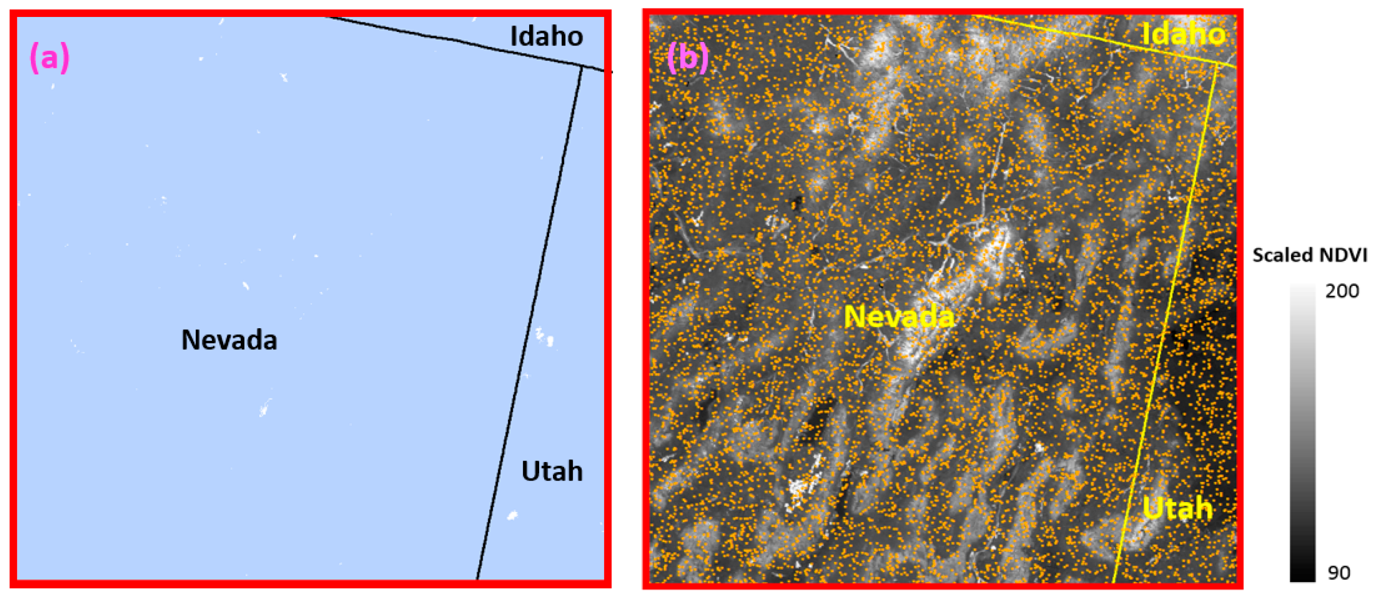
2.2.2. Landsat 8 Observations and MODIS NDVI Data

A LANDFIRE tile (r04c03), which is a composite made up of multiple Landsat 8 scenes for a target date, was selected in this study. To minimize any cloud and bad detection effects in the original Landsat 8 data, a compositing approach using cosine-similarity was used [45], which combines pixels from multiple observations based on data quality and temporal proximity to a target date. In this case, Julian date 212 which yielded relatively low “no data and/or cloudy” pixels, was used as the target date with observations from days 140–240 in 2013. The derived 30 m composite data were then upscaled to 250 m using the “spatial averaging” method [29]. Based on our previous study results [29,44], six Landsat 8 spectral bands (bands 1–6) at 250 m resolution were used as independent variables for developing the piecewise regression tree models to predict the 250 m MODIS NDVI (dependent variables). Furthermore, to ensure the high quality of the derived 250 m Landsat 8 data, and avoid any additional cloud and atmospheric effects, the percentage of 30-m pixel(s) with “0” value(s) within a 250 m pixel was calculated. Only those 250 m pixels with 0% of “0” values (i.e., all the 30 m pixels within a 250 m pixel are none “zero vales” pixels) were selected (Figure 2a, light blue color) to develop regression tree models.

The seven-day maximum value composites of 250-m MODIS NDVI (scaled NDVI, value from 0 to 200) for the year 2013 were obtained from the USGS expedited MODIS (eMODIS) data archive [46]. Pixels with bad quality, negative values, clouds, snow cover, and low view angles were filtered out based on the MODIS quality assurance data [47] to ensure high quality eMODIS NDVI data. The 2013 weekly NDVI data were then stacked and temporally smoothed using a weighted least-squares approach to reduce additional atmospheric noise [48]. Temporal smoothing helps to ensure reliable NDVI values for weekly or longer cloudy periods [49]. Finally, the 250 m MODIS NDVI for the date around Julian date 212 (similar date as the Landsat scene date) was extracted and used as the dependent variable in the regression tree model.

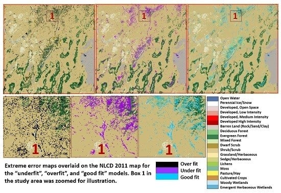
2.2.3. Spatial Evaluations of Large Model Prediction Errors Using NLCD 2011

The USGS 30-m NLCD 2011 map for the study area was obtained from the NLCD 2011 data archive [50] (Figure 1). This NLCD map was used to evaluate where and what land cover types are likely to have large prediction errors (i.e., over- and underfitting effects; see the next section for a detailed explanation) and investigate the potential cause of the large errors.

2.3. Method and Procedures

2.3.1. Method

As described earlier, the main goal and focus of this study is to develop an approach that identifies the optimal sample data usage strategy for regression tree models by minimizing over- and underfitting effects in the model. The mean absolute difference (MAD) between the predicted NDVI and the actual NDVI (scaled NDVI, value from 0–200) was calculated (Equation (1)) and used to evaluate model over- and underfitting tendencies. The standard deviation of the MAD (SD) from the nine different randomized tests using the same criteria for building the regression tree models was also calculated (Equation (2)) and used to assess regression tree model performance.

$$\mathrm{MAD}=\frac{1}{\mathrm{N}}{\displaystyle \sum }_{\mathrm{k}=1}^{\mathrm{N}}\mathrm{abs}({\mathrm{NDVI}}_{{\mathrm{predicted}}_{\mathrm{k}}}-{\mathrm{NDVI}}_{{\mathrm{actual}}_{\mathrm{k}}})$$

(1)

N: total number of samples.

$$\mathrm{SD}=\sqrt{\frac{1}{9}{\displaystyle \sum }_{\mathrm{i}=1}^9{({\mathrm{MAD}}_{\mathrm{i}}-{\mathrm{MAD}}_{\mathrm{mean}})}^2}$$

(2)

In this study, “underfitting” is defined as the highest errors (MAD) for both training and testing (i.e., validation), and “overfitting” means training error is low while testing error is high (i.e., MAD_training < MAD_testing). “Good fit” (i.e., optimal model) is defined as the lowest errors for both validation and training and with relatively low SD [32].

Table 1. Mean absolute difference (MAD) between predicted NDVI and actual NDVI and standard deviation of the MAD (SD) for regression tree model performance.

	Overfitting	Underfitting	Good Fit
MAD	MADtraining < MADtesting	Highest MADtraining and highest MADtesting	Lowest MADtraining and lowest MADtesting
SD	High	High	Relatively low

is a summary of the criteria used to assess regression tree model performance.

A series of tests was performed that include (1) small training data size with a large testing data size (large training and testing MADs were expected primarily from overgeneralization); (2) large training data size with small testing size (high testing MAD with relatively low training MAD were expected primarily from overfitting); and (3) the “happy medium” (robust model with minimal errors) with different maximum allowed number of rules to build Cubist regression tree models. Models with overfitting, underfitting, and good fit conditions were identified based on the criteria in Table 1.

2.3.2. Processing Procedures

Python is a programming language that allows a programmer to develop code (e.g., batch processing) and subsequently uses an interpreter to run the code [51]. A Python script was developed to automatically perform two Cubist modeling procedures (version 2.07 GPL Edition). The first procedure replicates a Cubist model nine times utilizing 10%–90% of the subsamples of a given dataset (i.e., training data) incrementally by 10%, resulting in a total of 81 model runs. Training data were randomly sampled from the entire dataset per 10% subsample. The maximum number of rules (i.e., regression trees) that could be used was set to 100 and the maximum extrapolation (values can range between 0 and 100%; increasing numbers indicate the percent adjustment of the rules to the training set) was set to 10%. The MAD and SD for both testing and training were subsequently calculated and were output as a summary file. The summary file also includes the minimum and maximum number of rules at each 10% increment. The second procedure held the random sampling percentage for training constant at a user-defined value (40%, 60%, and 80%), varied the number of rules between 1 and 100, and set the maximum extrapolation to 10%. The MAD was subsequently calculated for each of the rules. The following steps describe an application of this approach (a case study), demonstrating the detailed processing procedures of this method:

1. Classify the MODIS NDVI map into three classes (low, medium, and high NDVI) with each class having an equal amount of pixels. Selected ~10,000 randomly stratified samples from the study area based on the three NDVI classes (Figure 2b, each class had ~3330 random samples). The 250 m six-band Landsat 8 data (independent variables) and 250 m MODIS NDVI (dependent variable) were extracted for each of the selected samples [52].

2. Develop data-driven rule-based piecewise regression tree models using 10%, 20%, 30%, 40%, 50%, 60%, 70%, 80%, and 90% of the sample data as the model training data in Cubist (nine different randomized tests were run and nine models for each percentage were built). Mean training and testing MAD and SD from the nine randomized tests for each of the training data percentages were calculated and models with overfitting, underfitting, and good fit potentials (Table 1) were identified. All procedures were accomplished utilizing the above Python script.

3. Used different rule numbers (i.e., rule numbers from one to maximum observed rule numbers determined by Cubist regression tree algorithm, in our case, from 1–12) with the selected optimal percentage of sample training data (40%, 60%, and 80% from step 2 in this case study) to build the Cubist regression tree models. Calculated the MAD for each model and identified the optimal rule numbers that mitigate over- and underfitting effects and minimize the prediction errors.

4. Based on the results from steps 2 and 3, additional testing was performed to determine the final model parameters (percent of training data size and number of rules) for overfitting and underfitting models in this case study. These tests include (1) using 10% training data size (overfitting tendency) with different rule numbers (1–12 rules), and (2) using one rule (underfitting tendency) with different training data sizes (10%–90%) to build the Cubist regression tree models.

Additionally, the following procedures were performed in our case study application to quantify and understand the mapping impacts of overfitting, underfitting, good fit, and all sample prediction models:

A. Predicted the 250 m MODIS-Landsat NDVI using overfitting, underfitting, good fit, and all samples (100% of the samples used for model development) regression tree models. Mapped the absolute difference (AD) between the predicted NDVI and the actual NDVI for the study areas for each model. Since the scaled NDVI (value from 0–200) was used in this study, the AD and MAD values calculated from this study were also scaled (i.e., the real AD and MAD values should be divided by 100).

B. Generated the extreme AD (i.e., scaled AD > 10, real AD > 0.01) maps for the “overfit”, “underfit”, “good fit”, and “all samples” models. Compared the four extreme AD maps and investigated the potential causes (where and why) of the extreme AD based on the NLCD 2011 map.

C. Evaluated the MAD comparison graphics for the four models (overfit, underfit, good fit, and all samples) based on the three categories (i.e., MAD ≤ 10, MAD > 10, and all cases).

3. Results and Discussion

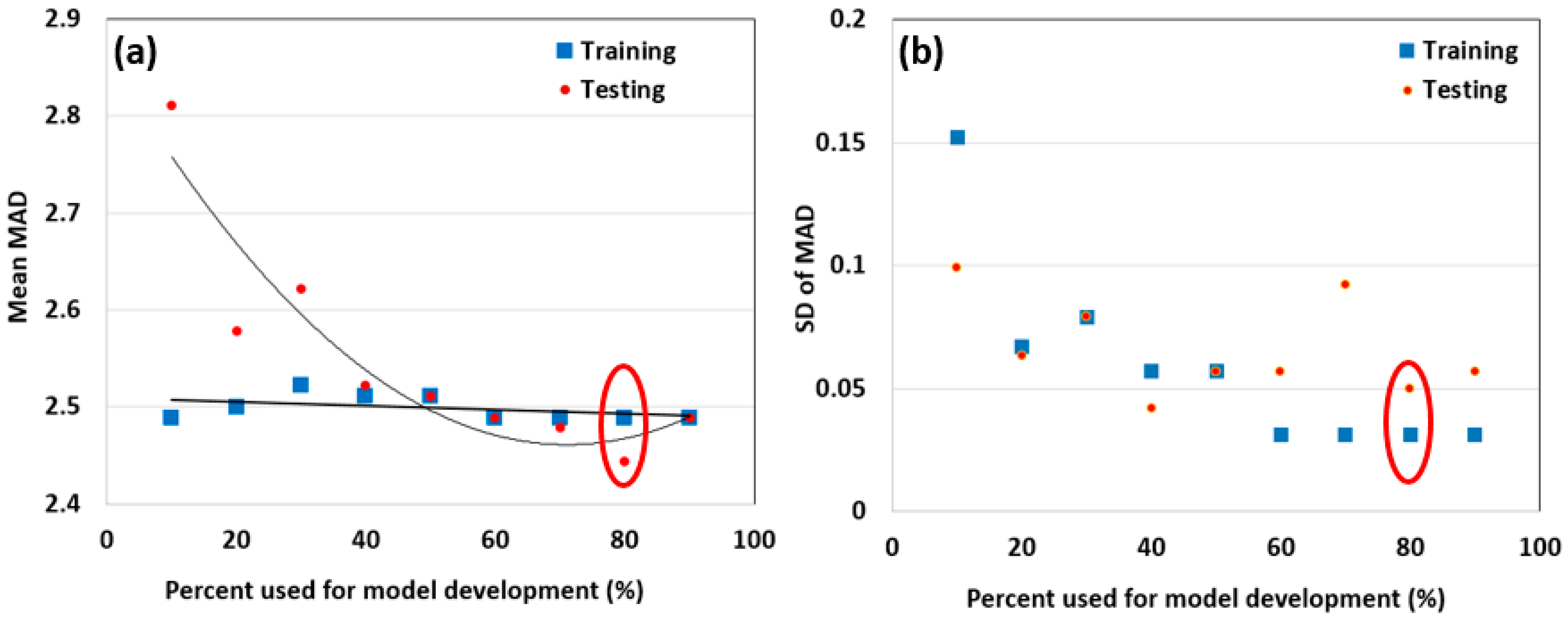
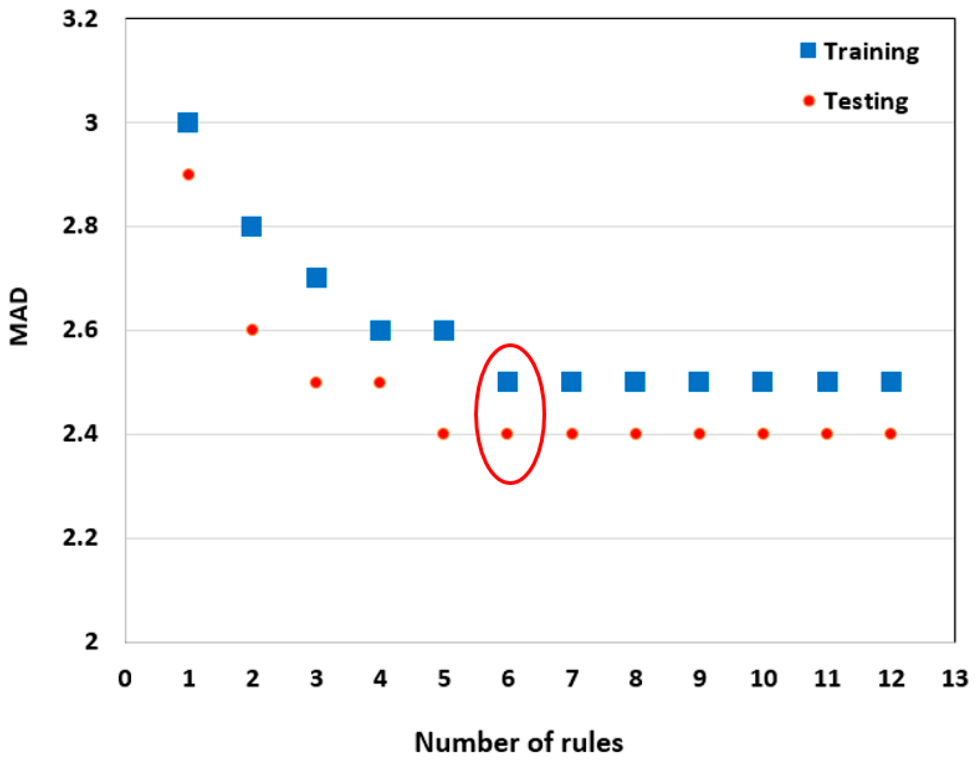
3.1. Identification of the Optimal Regression Tree Model Complexity and Associated Model Parameters

Results from the Cubist model replication tests (step 2) show that there are only minor differences in error observed across all of the training data sizes (Figure 3a, all mean values of MAD < 3), suggesting that Cubist was resistant to overfitting. The training MAD was constant across the gradient of training data sizes (blue color in Figure 3a), while the testing MAD was higher at low training data sizes, indicting improved model robustness with larger training sizes. The Cubist model derived from the 80% sample training data size had the lowest MAD and SD (red circles in Figure 3a,b) for both training and testing, indicating the optimal sample data usage for the regression tree model (Table 1). On the other hand, using a 10% training data size to develop the Cubist regression tree model, the MAD for testing is much higher than the MAD for training and the SDs for both training and testing are high (Figure 3), indicating an overfitting tendency in these models (Table 1).

To further optimize the rule numbers, regression tree models were built using 80% of the sample data with varying maximum number of rules from 1–12 (processing step 3). Results show that the MADs for both training and testing were stable when the rule number was greater than approximately six (Figure 4). Therefore in this case study, we concluded that an accurate and parsimonious model occurred at the 80% training data size with six rules (MAD_training =2.5 and MAD_testing = 2.4). Furthermore, the validation error (testing error) is expected to be reliable and consistent (the testing SD was low for the 80% training data size model replications, Figure 3b). Description of this optimal regression tree model (6 rules) can be found from the “Supplementary Materials”.

Based on the rule number tests in processing steps 3 and 4 (Figure 4), we found that the regression tree models with one rule resulted in large MAD for both training and testing (ranges from 2.9–3.1), which indicated an underfitting tendency in these models. In this case study, using 40% of the data for training with one rule in the regression tree model (MAD_training =3.0 and MAD_testing =3.0) met our criteria for the underfitting condition (Table 1). In addition, a Cubist model trained on 10% of the sample data with 11 rules in the regression tree model (MAD_training =2.2 and MAD_testing =2.8) was used as an example for the overfitting condition.

3.2. Model Accuracy Assessments for the Four Conditions

To provide a clear view of how the MADs varied through the “overfit”, “underfit”, “good fit”, and all samples in the regression tree models, the MAD histograms for the three AD categories (all AD; low error with AD ≤10; and high error with AD >10) are illustrated in Figure 5a. Both “good fit” and “all samples” have the lowest MADs when compared with “overfit” and “underfit” model predictions. Since independent testing data are desirable to quantify the model error rates, in this case study the “good fit” model was considered as the “best” model, which optimized both model parameters (number of rules) and sample data usage (suitable portion for training and testing) compared with the “all samples” model.

The “underfit” model had the highest overall MAD (Figure 5a) and a slightly higher frequency of occurrence in the AD ≤10 class than the “overfit” model (Figure 5b). This suggests that the prediction errors from the “underfit” model generally occurred within the low error group. Within the large error (AD > 10) category, the “overfit” model had a slightly higher MAD than the “underfit” model (Figure 5a), but it also had the highest frequency of occurrence in comparison with the other models (Figure 5b), implying that the “overfit” model tends to produce larger magnitudes of errors (or large outliers) than the other models. The “overfit” model may develop rules based on the noise signals within the training data or develop over-specific, non-robust rulesets, resulting in a tendency for more frequent extreme errors in model predictions.

The “all sample” and the “good fit” models have the lowest overall AD (Figure 5a), the most frequent perfect predictions (i.e., AD = 0), and the least frequent large errors (AD > 10) compared with the other model predictions (Figure 5b). The “overfit” model had over-specified conditions, which had a tendency to either predict very well (i.e., AD = 0) or very poorly (frequency of AD >10) across the study area. In general, the “overfit” model, with its limited robustness, performed better than the “underfit” model (low overall AD in Figure 5a). It appears that the model diagnostic approach proposed in this study can successfully identify the “overfit”, “underfit”, and “good fit” models.

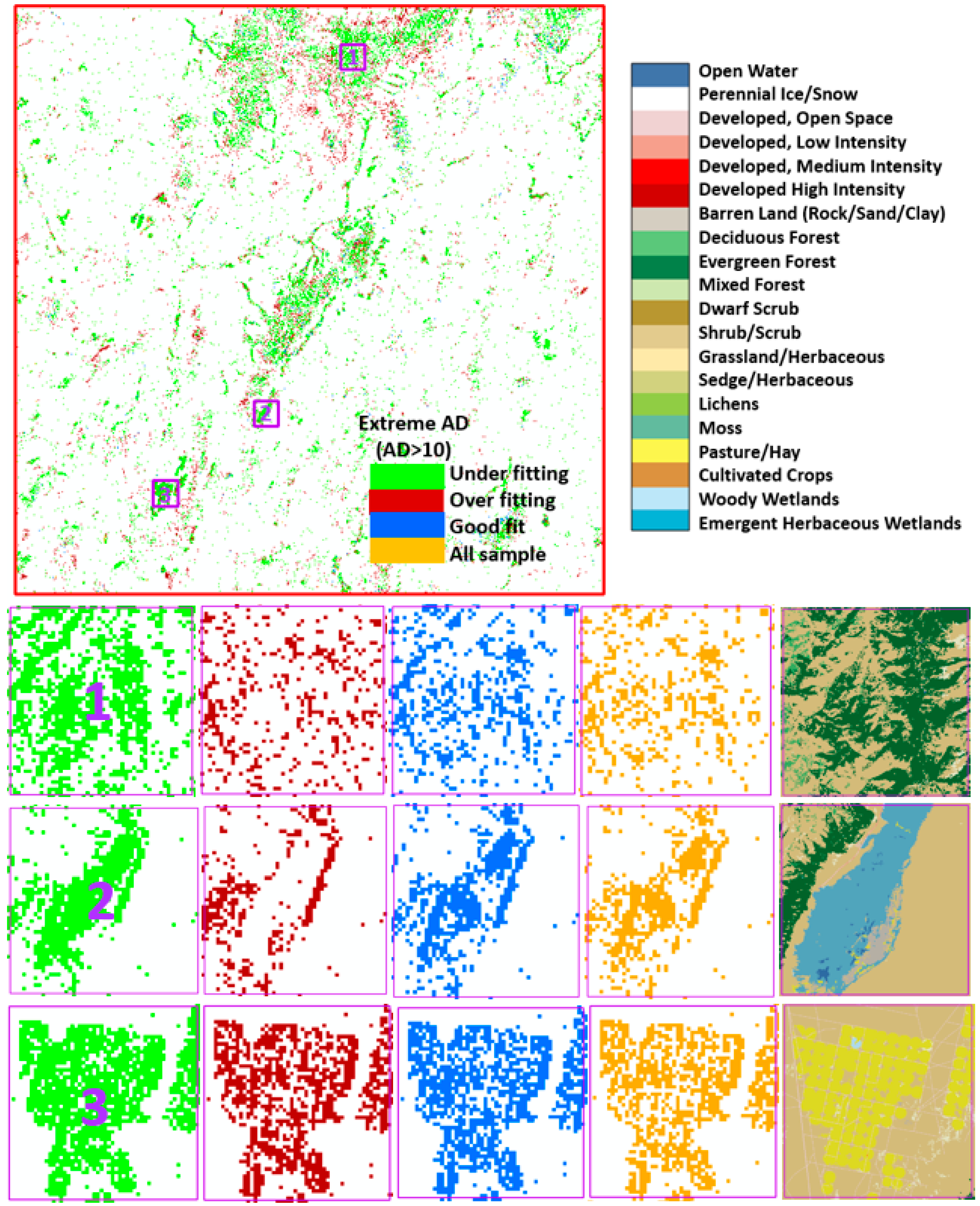
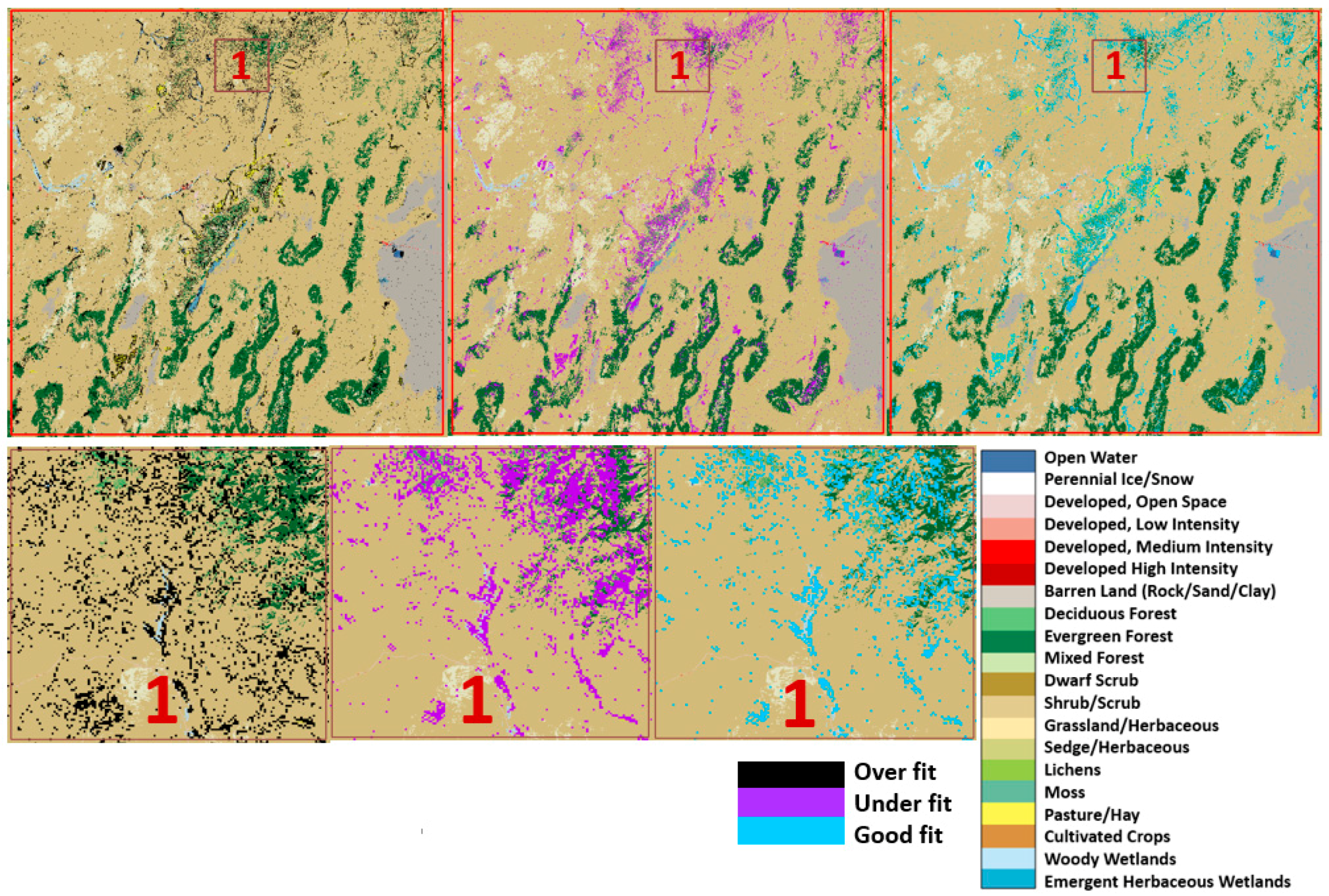
3.3. Evaluation of the Extreme AD Regions for the Four Models Using NLCD 2011

To understand and demonstrate the prediction errors in a mapping application, locations and land cover types for the large prediction error pixels (AD > 10) from the four models (“underfit”, “overfit”, “good fit”, and all samples) were mapped for the study area (Figure 6). Three boxes representing different locations with large numbers of high AD pixels were selected for evaluation. The extreme AD maps from the four models with 30 m land cover type (NLCD 2011) maps for the three boxes are illustrated in Figure 6 boxes 1–3. Results show that pixels with large prediction errors (particularly for the overfitting model) are usually mixed land cover types (within a 250 m model training resolution) and located along the edges of riparian zones, croplands, and forests (Figure 6, boxes 1–3). Mixed land cover types within 250 m pixels can confound satellite spectral signals and lead to large model prediction errors. These same mixed pixel errors would also exist in the 30 m land cover product used in this study. The locations and the spatial patterns of the large AD regions are similar for the four models; however, differences can still be found especially for the “underfit” model. For example, there are more extreme high AD pixels within boxes 1 and 2 (Figure 6) from the “underfit” model than the other models, implying that the “underfit” model is less reliable in these regions than the other models.

3.4. Discussion

Overall, there were only minor differences in accuracy across all the models. Results from this case study indicate that Cubist software was generally quite resistant to overfitting and underfitting tendencies. The generalization of the regression tree into “rules” by Cubist helps mitigate overfitting effects [27]. The mean absolute error modified by the ratio of the number of cases and the number of parameters is the cost function employed by Cubist, which weighs the process toward having fewer parameters and trying to simplify the model as a whole. This function is used in both parameter elimination during the regression fitting and pruning the regression trees. In our case study, the model accuracy was stable with rule numbers greater than five (Figure 4). However, different datasets may vary in the optimal number of rules and training to testing data size ratios needed for the regression tree model. Our approach, which could be applied to other Cubist modeling applications, is to identify a parsimonious number of rules and training to testing data size ratios to minimize the prediction errors.

As described in Section 3.2, both the “good fit” and “all samples” models have the lowest MADs. The “good fit” model was selected as the “best” model in this case study to allow the quantification of model errors. However, when the reference data (sample data) are limited and maximizing model accuracy while mitigating overfitting tendencies is important (e.g., carbon flux mapping based on observations from several flux towers), the “best” model is suggested to be developed from all of the available sample points. Using leave-one-out cross-validation [26,53], random k-fold validation [54,55,56,57], or randomized test replication methods can provide reasonable error rate expectations on unseen data (particularly if testing accuracies are stable over multiple replications).

Although the locations and the spatial patterns of the large AD error regions are similar for the four models, differences can still be found, especially for the “underfit” and the “overfit” models. Figure 7 shows the extreme AD (AD > 10) maps overlaid on the NLCD 2011 land cover for the “overfit” (black), “underfit” (magenta), and “good fit” (light blue) models. Additionally, a small box in the study area was selected and zoomed for illustration (Figure 7). The extreme AD regions for the “underfit” model usually occurred along ecotones, while the “overfit” model had more outliers (large errors) in the middle of the rangelands, indicating tight data space envelopes from the training data for rangelands are being exceeded in the rangeland population being mapped (Figure 7). The “good fit” model had fewer extreme AD pixels than the other two models (Figure 5b and Figure 7).

4. Conclusions

This study developed a Cubist model optimization approach that uses variation in training sizes and rule numbers to identify combinations that minimize over- and underfitting effects on unseen data and improve the accuracy and robustness of the Cubist model. Our case study demonstrated that using 80% of the data as the training data (saving 20% of the data as independent test) with six rules in the regression tree model had the lowest prediction errors (MAD_training = 2.5 and MAD_testing = 2.4) (the scaled NDVIs with values from 0–200 were used in this study) and was chosen as the “good fit” (or optimal) model. However, when the sample data size is limited and maximizing model accuracy is a high priority (e.g., carbon flux mapping based on observations from several flux towers), using all the available data to build the Cubist model and employing a cross-validation accuracy assessment method is recommended to maximize model robustness for unseen data.

Using 10% of the sample data as the model training data with 11 rules in the regression tree model has relatively low MAD for training but high MAD for testing (MAD_training = 2.2 and MAD_testing = 2.8), which was considered an “overfit” model. When 40% of the sample data was used as training data with one rule in the regression tree model, the MADs are high for both training and testing (MAD_training = 3.0 and MAD_testing = 3.0) and was considered an “underfit” model in this case study. Results from this study provide useful information on how the training data selection impacts the accuracy of the regression tree model and which data usage strategy can minimize the model overfitting and underfitting impacts. This regression tree model optimization approach will be useful for future remote-sensing-based ecosystem parameter (e.g., biomass, cover, and carbon flux) mapping.

References

1. Anderson, J.R.; Hardy, E.E.; Roach, J.T.; Witmer, R.E. A Land Use and Land Cover Classification System for Use with Remote Sensor Data; P 0964; U.S. Geological Survey: Reston, VA, USA, 1976; p. 28.
2. Gu, Y.; Brown, J.F.; Miura, T.; van Leeuwen, W.J.; Reed, B.C. Phenological classification of the United States: A geographic framework for extending multi-sensor time-series data. Remote Sens. 2010, 2, 526–544. [Google Scholar] [CrossRef]
3. Wylie, B.K.; Zhang, L.; Bliss, N.B.; Ji, L.; Tieszen, L.L.; Jolly, W.M. Integrating modelling and remote sensing to identify ecosystem performance anomalies in the boreal forest, Yukon River Basin, Alaska. Int. J. Digit. Earth 2008, 1, 196–220. [Google Scholar] [CrossRef]
4. Gu, Y.; Wylie, B.K. Detecting ecosystem performance anomalies for land management in the upper colorado river basin using satellite observations, climate data, and ecosystem models. Remote Sens. 2010, 2, 1880–1891. [Google Scholar] [CrossRef]
5. Homer, C.; Dewitz, J.; Yang, L.; Jin, S.; Danielson, P.; Xian, G.; Coulston, J.; Herold, N.; Wickham, J.; Megown, K. Completion of the 2011 national land cover database for the conterminous United States–representing a decade of land cover change information. Photogramm. Eng. Remote Sens. 2015, 81, 345–354. [Google Scholar]
6. Homer, C.G.; Aldridge, C.L.; Meyer, D.K.; Schell, S.J. Multi-scale remote sensing sagebrush characterization with regression trees over wyoming, USA: Laying a foundation for monitoring. Int. J. Appl. Earth Obs. Geoinf. 2012, 14, 233–244. [Google Scholar] [CrossRef]
7. Peters, A.J.; Walter-Shea, E.A.; Ji, L.; Viña, A.; Hayes, M.; Svoboda, M.D. Drought monitoring with ndvi-based standardized vegetation index. Photogramm. Eng. Remote Sens. 2002, 68, 71–75. [Google Scholar]
8. Potter, C.S.; Randerson, J.T.; Field, C.B.; Matson, P.A.; Vitousek, P.M.; Mooney, H.A.; Klooster, S.A. Terrestrial ecosystem production: A process model based on global satellite and surface data. Glob. Biogeochem. Cycles 1993, 7, 811–841. [Google Scholar] [CrossRef]
9. Tucker, C.J.; Vanpraet, C.L.; Sharman, M.J.; van Ittersum, G. Satellite remote sensing of total herbaceous biomass production in the senegalese sahel: 1980–1984. Remote Sens. Environ. 1985, 17, 233–249. [Google Scholar] [CrossRef]
10. Reed, B.C.; Brown, J.F.; Vanderzee, D.; Loveland, T.R.; Merchant, J.W.; Ohlen, D.O. Measuring phenological variability from satellite imagery. J. Veg. Sci. 1994, 5, 703–714. [Google Scholar] [CrossRef]
11. Loveland, T.R.; Reed, B.C.; Brown, J.F.; Ohlen, D.O.; Zhu, Z.; Yang, L.; Merchant, J.W. Development of a global land cover characteristics database and IGBP DISCover from 1 km AVHRR data. Int. J. Remote Sens. 2000, 21, 1303–1330. [Google Scholar] [CrossRef]
12. Washington-Allen, R.A.; West, N.E.; Ramsey, R.D.; Efroymson, R.A. A protocol for retrospective remote sensing-based ecological monitoring of rangelands. Rangel. Ecol. Manag. 2006, 59, 19–29. [Google Scholar] [CrossRef]
13. Burgan, R.E.; Klaver, R.W.; Klarer, J.M. Fuel models and fire potential from satellite and surface observations. Int. J. Wildland Fire 1998, 8, 159–170. [Google Scholar] [CrossRef]
14. Zhu, Z.; Woodcock, C.E. Continuous change detection and classification of land cover using all available Landsat data. Remote Sens. Environ. 2014, 144, 152–171. [Google Scholar] [CrossRef]
15. Chen, J.; Chen, J.; Liao, A.; Cao, X.; Chen, L.; Chen, X.; He, C.; Han, G.; Peng, S.; Lu, M.; et al. Global land cover mapping at 30 m resolution: A pok-based operational approach. ISPRS J. Photogramm. Remote Sens. 2015, 103, 7–27. [Google Scholar] [CrossRef]
16. Giri, C.; Pengra, B.; Long, J.; Loveland, T.R. Next generation of global land cover characterization, mapping, and monitoring. Int. J. Appl. Earth Obs. Geoinform. 2013, 25, 30–37. [Google Scholar] [CrossRef]
17. Reed, B.C.; White, M.A.; Brown, J.F. Remote sensing phenology. In Phenology: An Integrative Environmental Science; Schwartz, M.D., Ed.; Kluwer Academic Publ.: Dordrecht, The Netherlands, 2003; pp. 365–381. [Google Scholar]
18. Tan, Z.; Liu, S.; Wylie, B.K.; Jenkerson, C.B.; Oeding, J.; Rover, J.; Young, C. MODIS-informed greenness responses to daytime land surface temperature fluctuations and wildfire disturbances in the Alaskan Yukon River Basin. Int. J. Remote Sens. 2012, 34, 2187–2199. [Google Scholar] [CrossRef]
19. White, M.A.; de Beurs, K.M.; Didan, K.; Inouye, D.W.; Richardson, A.D.; Jensen, O.P.; O’Keefe, J.; Zhang, G.; Nemani, R.R.; van Leeuwen, W.J.D.; et al. Intercomparison, interpretation, and assessment of spring phenology in North America estimated from remote sensing for 1982–2006. Glob. Chang. Biol. 2009, 15, 2335–2359. [Google Scholar] [CrossRef]
20. Becker-Reshef, I.; Vermote, E.; Lindeman, M.; Justice, C. A generalized regression-based model for forecasting winter wheat yields in Kansas and Ukraine using MODIS data. Remote Sens. Environ. 2010, 114, 1312–1323. [Google Scholar] [CrossRef]
21. Howard, D.M.; Wylie, B.K.; Tieszen, L.L. Crop classification modelling using remote sensing and environmental data in the greater Platte River Basin, USA. Int. J. Remote Sens. 2012, 33. [Google Scholar] [CrossRef]
22. Wylie, B.K.; Boyte, S.P.; Major, D.J. Ecosystem performance monitoring of rangelands by integrating modeling and remote sensing. Rangel. Ecol. Manag. 2012, 65. [Google Scholar] [CrossRef]
23. Park, S.; Im, J.; Jang, E.; Rhee, J. Drought assessment and monitoring through blending of multi-sensor indices using machine learning approaches for different climate regions. Agric. Forest Meteorol. 2016, 216, 157–169. [Google Scholar] [CrossRef]
24. Yang, F.; Ichii, K.; White, M.A.; Hashimoto, H.; Michaelis, A.R.; Votava, P.; Zhu, A.X.; Huete, A.; Running, S.W.; Nemani, R.R. Developing a continental-scale measure of gross primary production by combining MODIS and ameriflux data through support vector machine approach. Remote Sens. Environ. 2007, 110, 109–122. [Google Scholar] [CrossRef]
25. Xiao, J.; Zhuang, Q.; Law, B.E.; Chen, J.; Baldocchi, D.D.; Cook, D.R.; Oren, R.; Richardson, A.D.; Wharton, S.; Ma, S.; et al. A continuous measure of gross primary production for the conterminous United States derived from MODIS and ameriflux data. Remote Sens. Environ. 2010, 114, 576–591. [Google Scholar] [CrossRef]
26. Zhang, L.; Wylie, B.K.; Ji, L.; Gilmanov, T.G.; Tieszen, L.L.; Howard, D.M. Upscaling carbon fluxes over the great plains grasslands: Sinks and sources. J. Geophys. Res. Biogeosci. 2011, 116. [Google Scholar] [CrossRef]
27. RuleQuest Research. Available online: http://www.rulequest.com/ (accessed on 10 November 2016).
28. Zhang, L.; Wylie, B.K.; Ji, L.; Gilmanov, T.G.; Tieszen, L.L. Climate-driven interannual variability in net ecosystem exchange in the Northern Great Plains Grasslands. Rangel. Ecol. Manag. 2010, 63, 40–50. [Google Scholar] [CrossRef]
29. Gu, Y.; Wylie, B. Downscaling 250-m MODIS growing season NDVI based on multiple-date Landsat images and data mining approaches. Remote Sens. 2015, 7, 3489–3506. [Google Scholar] [CrossRef]
30. Boyte, S.P.; Wylie, B.K.; Major, D.J.; Brown, J.F. The integration of geophysical and enhanced moderate resolution imaging spectroradiometer normalized difference vegetation index data into a rule-based, piecewise regression-tree model to estimate cheatgrass beginning of spring growth. Int. J. Digit. Earth 2013, 8. [Google Scholar] [CrossRef]
31. Brown, J.F.; Wardlow, B.D.; Tadesse, T.; Hayes, M.J.; Reed, B.C. The vegetation drought response index (vegdri): A new integrated approach for monitoring drought stress in vegetation. GISci. Remote Sens. 2008, 45, 16–46. [Google Scholar] [CrossRef]
32. Hastie, T.; Tibshirani, R.; Friedman, J. The Elements of Statistical Learning: Data Mining, Inference, and Prediction, 2nd ed.; Springer: New York, NY, USA, 2009. [Google Scholar]
33. Smale, C. Best choices for regularization parameters in learning theory: On the bias—Variance problem. Found. Comput. Math. 2002, 2, 413–428. [Google Scholar]
34. Yu, L.; Lai, K.K.; Wang, S.; Huang, W. A bias-variance-complexity trade-off framework for complex system modeling. In Computational Science and Its Applications—ICCSA 2006: International Conference, Glasgow, Uk, 8–11 May 2006. Proceedings, Part I; Gavrilova, M., Gervasi, O., Kumar, V., Tan, C.J.K., Taniar, D., Laganá, A., Mun, Y., Choo, H., Eds.; Springer: Berlin/Heidelberg, Germany, 2006; pp. 518–527. [Google Scholar]
35. Quinlan, J.R. Combining instance-based and model-based learning. In Proceedings of the Tenth International Conference on Machine Learning, Amherst, MA, USA, 27–29 June 1993; pp. 236–243.
36. Rouse, J.W., Jr.; Haas, H.R.; Deering, D.W.; Schell, J.A.; Harlan, J.C. Monitoring the Vernal Advancement and Retrogradation (Green Wave Effect) of Natural Vegetation; NTRS: Greenbelt, MD, USA, 1974; p. 371. [Google Scholar]
37. Tucker, C.J. Red and photographic infrared linear combinations for monitoring vegetation. Remote Sens. Environ. 1979, 8, 127–150. [Google Scholar] [CrossRef]
38. Chen, D.; Brutsaert, W. Satellite-sensed distribution and spatial patterns of vegetation parameters over a Tallgrass Prairie. J. Atmos. Sci. 1998, 55, 1225–1238. [Google Scholar] [CrossRef]
39. Funk, C.; Budde, M.E. Phenologically-tuned MODIS NDVI-based production anomaly estimates for Zimbabwe. Remote Sens. Environ. 2009, 113, 115–125. [Google Scholar] [CrossRef]
40. Gu, Y.; Wylie, B.K.; Bliss, N.B. Mapping grassland productivity with 250-m emodis NDVI and ssurgo database over the greater Platte River Basin, USA. Ecol. Indic. 2013, 24, 31–36. [Google Scholar] [CrossRef]
41. MODIS Products Table. Available online: https://lpdaac.usgs.gov/dataset_discovery/modis/modis_products_table (accessed on 10 November 2016).
42. Tieszen, L.L.; Reed, B.C.; Bliss, N.B.; Wylie, B.K.; DeJong, D.D. NDVI, C3 and C4 production, and distributions in Great Plains grassland land cover classes. Ecol. Appl. 1997, 7, 59–78. [Google Scholar]
43. Wylie, B.K.; Denda, I.; Pieper, R.D.; Harrington, J.A.; Reed, B.C.; Southward, G.M. Satellite-based herbaceous biomass estimates in the pastoral zone of Niger. J. Range Manag. 1995, 48, 159–164. [Google Scholar] [CrossRef]
44. Gu, Y.; Wylie, B.K. Developing a 30-m grassland productivity estimation map for Central Nebraska using 250-m MODIS and 30-m Landsat-8 observations. Remote Sens. Environ. 2015, 171, 291–298. [Google Scholar] [CrossRef]
45. Nelson, K.J.; Steinwand, D. A Landsat data tiling and compositing approach optimized for change detection in the conterminous United States. Photogramm. Eng. Remote Sens. 2015, 81, 573–586. [Google Scholar] [CrossRef]
46. USGS eMODIS Data. Available online: https://lta.cr.usgs.gov/emodis (accessed on 10 November 2016).
47. Jenkerson, C.B.; Maiersperger, T.K.; Schmidt, G.L. Emodis—A User-Friendly Data Source; U.S. Geological Survey Open-File Report 2010-1055; U.S. Geological Survey Earth Resources Observation and Science (EROS) Center: Sioux Falls, SD, USA, 2010.
48. Swets, D.L.; Reed, B.C.; Rowland, J.R.; Marko, S.E. A weighted least-squares approach to temporal smoothing of NDVI. In Proceedings of the ASPRS Annual Conference, From Image to Information, Portland, Oregon, 17–21 May 1999.
49. Brown, F.J.; Howard, D.; Wylie, B.; Frieze, A.; Ji, L.; Gacke, C. Application-ready expedited MODIS data for operational land surface monitoring of vegetation condition. Remote Sens. 2015, 7, 16226–16240. [Google Scholar] [CrossRef]
50. National Land Cover Database 2011. Available online: http://www.mrlc.gov/nlcd2011.php (accessed on 10 November 2016).
51. Python Software Foundation. Available online: https://www.python.org/ (accessed on 10 November 2016).
52. Gu, Y.; Wylie, B.K.; Boyte, S.P. Landsat 8 Six Spectral Band Data and MODIS NDVI Data for Assessing the Optimal Regression Tree Models. Available online: https://dx.doi.org/10.5066/F7319T1P (accessed on 10 November 2016).
53. Cawley, G.C.; Talbot, N.L.C. Fast exact leave-one-out cross-validation of sparse least-squares support vector machines. Neural Netw. 2004, 17, 1467–1475. [Google Scholar] [CrossRef] [PubMed]
54. Wylie, B.K.; Johnson, D.A.; Laca, E.A.; Saliendra, N.Z.; Gilmanov, T.G.; Reed, B.C.; Tieszen, L.L.; Worstell, B.B. Calibration of remotely sensed, coarse resolution NDVI to co 2 fluxes in a sagebrush-steppe ecosystem. Remote Sens. Environ. 2003, 85, 243–255. [Google Scholar] [CrossRef]
55. Wylie, B.K.; Fosnight, E.A.; Gilmanov, T.G.; Frank, A.B.; Morgan, J.A.; Haferkamp, M.R.; Meyers, T.P. Adaptive data-driven models for estimating carbon fluxes in the Northern Great Plains. Remote Sens. Environ. 2007, 106, 399–413. [Google Scholar] [CrossRef]
56. Ji, L.; Wylie, B.K.; Nossov, D.R.; Peterson, B.E.; Waldrop, M.P.; McFarland, J.W.; Rover, J.A.; Hollingsworth, T.N. Estimating aboveground biomass in interior alaska with Landsat data and field measurements. Int. J. Appl. Earth Obs. Geoinf. 2012, 18, 451–461. [Google Scholar] [CrossRef]
57. Xiao, J.; Ollinger, S.V.; Frolking, S.; Hurtt, G.C.; Hollinger, D.Y.; Davis, K.J.; Pan, Y.; Zhang, X.; Deng, F.; Chen, J.; et al. Data-driven diagnostics of terrestrial carbon dynamics over North America. Agric. For. Meteorol. 2014, 197, 142–157. [Google Scholar] [CrossRef]
Figure 1. Land cover types as identified by the 2011 National Land Cover Database [5] and the location of the study area (red box in the USA map). The legend is for the entire USA, some land cover types are not present within the study area.
Remotesensing 08 00943 g001
Figure 2. (a) Two-hundred fifty meter pixels with 0% of “0” values (light blue color) used to develop regression tree models and (b) randomly stratified samples (orange dots) overlaid on the 250 m MODIS NDVI (scaled NDVI, value from 0–200) map for the study area.
Remotesensing 08 00943 g002
Figure 3. (a) Mean MAD and (b) SD of MAD for the training and testing (validation) results from step 2. Eighty percent of the sample data used for training is highlighted by the red oval.
Remotesensing 08 00943 g003
Figure 4. Training and testing MAD based on the different number of rules for the 80% training data size. The red oval indicates the optimal number of rules and the associated training and testing MAD.
Remotesensing 08 00943 g004
Figure 5. (a) MAD values for all error (all AD), small error (AD ≤ 10), and large error (AD > 10, the MAD value for this class was scaled to get a better view with the other classes) categories based on the different model accuracy conditions; (b) percent of the total population (map area) for perfect prediction (AD = 0), small error (AD ≤ 10, % of total value was scaled to get a better view with the other classes), and large error (AD > 10) categories based on the different model accuracy conditions.
Remotesensing 08 00943 g005
Figure 6. Extreme AD (AD > 10 at 250 m resolution) map from the four models (underfit, overfit, good fit, and all samples) for the study area. Three small representative boxes (boxes 1–3) were selected and zoomed for MADs and 30 m NLCD 2011.
Remotesensing 08 00943 g006
Figure 7. Extreme AD maps overlaid on the NLCD 2011 map for the “underfit”, “overfit”, and “good fit” models. Box 1 in the study area was zoomed for illustration.
Remotesensing 08 00943 g007