Environmental and Anthropogenic Degradation of Vegetation in the Sahel from 1982 to 2006

Abstract

There is a great deal of debate on the extent, causes, and even the reality of land degradation in the Sahel. Investigations carried out before approximately 2000 using remote sensing data suggest widespread reductions in biological productivity, while studies extending beyond 2000 consistently reveal a net increase in vegetation production, strongly related to the recovery of rainfall following the extreme droughts of the 1970s and 1980s, and thus challenging the notion of widespread, long-term, subcontinental-scale degradation. Yet, the spatial variations in the rates of vegetation recovery are not fully explained by rainfall trends. It is hypothesized that, in addition to rainfall, other meteorological variables and human land use have contributed to vegetation dynamics. Throughout most of the Sahel, the interannual variability in growing season ΣNDVI_gs (measured from satellites, used as a proxy of vegetation productivity) was strongly related to rainfall, humidity, and temperature (mean r² = 0.67), but with rainfall alone was weaker (mean r² = 0.41). The mean and upper 95th quantile (UQ) rates of change in ΣNDVI_gs in response to climate were used to predict potential ΣNDVI_gs—that is, the ΣNDVI_gs expected in response to climate variability alone, excluding any anthropogenic effects. The differences between predicted and observed ΣNDVI_gs were regressed against time to detect any long-term (positive or negative) trends in vegetation productivity. Over most of the Sahel, the trends did not significantly depart from what is expected from the trends in meteorological variables. However, substantial and spatially contiguous areas (~8% of the total area of the Sahel) were characterized by negative, and, in some areas, positive trends. To explore whether the negative trends were human-induced, they were compared with the available data of population density, land use, and land biophysical properties that are known to affect the susceptibility of land to degradation. The spatial variations in the trends of the residuals were partly related to soils and tree cover, but also to several anthropogenic pressures.

1. Introduction

Since the 1990s, the human population in the Sahelian and Sudanian ecoclimatic zones (collectively referred to here as the “Sahel”) increased from approximately 120 million to over 280 million [1]. Population growth has been accompanied with cropland expansion and agricultural intensification [2,3,4], and with an increase in livestock numbers, from approximately 200 to over 430 million [5,6]. These changes coincided with two sequences of extremely dry years in 1972–1973 and again in 1983–1984 that were part of a longer drought that lasted from the end of the 1960s to the mid-1990s [7,8].

Coincident with intensification in land use and with the 1970s–1980s droughts, were noticeable reductions in vegetation productivity [9] and numerous studies, albeit local in scale, have reported cases of land degradation (e.g., [10,11,12]). These, plus anecdotal accounts of a progressive southwards march of the Sahara Desert [13,14], led to the popular view that population growth in the predominantly agrarian economies of the Sahelian countries was causing an extension of cultivation into marginal lands, shortened fallow periods, increased grazing intensity, and increased fuel-wood extraction, and that these population pressures coupled with the prolonged drought had caused widespread land degradation [15].

The existence of such widespread degradation has been challenged in a growing number of case studies that have found significant local variations in the relation between the increasing food demands, changes in land use patterns, and land degradation (e.g., [16,17,18,19]). It has been demonstrated that, under certain conditions, the standard degradation scenario has not occurred, owing to agricultural intensification and the emergence of mixed crop-livestock farming systems [20], and, furthermore, different measurement techniques have often resulted in different conclusions [21]. To date, the existence, causes, extent, and severity of land degradation throughout the Sahel remain controversial [22,23,24,25].

In contrast to the widespread belief in dryland degradation (“desertification”) of the Sahel, analysis of multitemporal satellite data from the 1990s onwards has revealed a consistent trend of vegetation recovery from the extreme droughts of the 1970s and early 1980s [26,27,28,29,30,31], suggesting that the perceived widespread degradation in the Sahel can largely be attributed to climate variability and not to irreversible changes in land productivity [28,30,32]. Currently, there is little if any evidence that the Sahelian drought alone (i.e., independent from human utilization of the land) has caused any land degradation [15]. Thus, it seems logical to distinguish between the effects of drought, which are temporary, and human-induced land degradation, which may have a trend of increasing severity, and can reach an end point of degradation that is usually long-term and even irreversible. The management implications for even extreme drought are very different to a system that will never return to its former state once climatological norms return [33].

The term land degradation is taken here to refer to the process by which less-productive biophysical conditions emerge owing to the excessive utilization of land with respect to its resilience [33]. Since net primary production (NPP) provides the energy that drives most biotic processes on Earth, persistent reductions in NPP from its potential—that is, the NPP expected in response to climate variability alone, excluding any human-induced changes in productivity—provides a useful indicator for land degradation monitoring [32,33,34]. This definition also serves to distinguish drought, in which vegetation and edaphic factors fully recover from a temporary reduction in rainfall, and land degradation, in which, over time, there is incomplete recovery [35] . It is important to note, however, that negative or positive trends in vegetation production relative to its potential are not necessarily the result of land degradation or land improvement as they can be caused by other factors including changes in land use, agricultural intensification, and CO₂ fertilization, among others. Therefore, negative trends only highlight potentially degrading areas where further examination is necessary to confirm the diagnosis [30,33,36]. However, in drylands, interannual variation in NPP is dominated by meteorological conditions, particularly by erratic rainfall [37], which mask more subtle and gradual changes such as degradation [36]. Thus, it is difficult to interpret trends in NPP without first accounting for the effects of meteorological variability on productivity [38].

A key requirement for detection of degradation is the availability of a reference—often the potential or non-degraded condition [39,40,41]. However, such sites are rarely known a priori, hence detection techniques are needed. Process-based, prognostic vegetation models (e.g., BIOME-BGC [42], LPJ-DVGM [43]) can estimate potential NPP for entire regions, however, the scarcity and coarse resolution of the necessary input data [44] and the requirement for many parameters, some complex (e.g., quantitative measures of the outcome of competition between plant functional types), largely exclude this type of model except for spatially uniform vegetation—an unusual occurrence. Furthermore, no existing process models can simulate human disturbance of the sort associated with degradation.

The method employed here uses NPP estimated using a light use efficiency approach in which satellite measurements of spectral reflectance are used to calculate the normalized difference vegetation index (NDVI), which is then summed over each growing season (ΣNDVI_gs). The potential, or non-degraded NPP is inferred from the observed relationship of ΣNDVI_gs and rainfall by regression—that is the rain-use efficiency (RUE, [32]). This method is an example of diagnostic, data-oriented, sometimes called “top-down” modeling. An important strength is that comparisons with the reference are made for each individual site, so differences between sites in unaccounted factors (such as soil differences) are normalized, allowing direct inter-site comparison. It can also be used at scales from local to global. However, the use of RUE in its simple form is subject to some important preconditions (

Table 1. Preconditions for valid application of Rain Use Efficiency (RUE) for detection of dryland degradation.

Precondition Number	Precondition
i	NPP must be primarily and linearly related to rainfall [32,45]
ii	NPP responds to rainfall within the current year with no carry-over from earlier years
iii	There are no supplements to current season rainfall, for example run-on from neighboring areas
iv	Within-season temporal patterns of rainfall do not affect NPP
v	The rainfall–NPP relationship does not vary between wet and dry years
vi	Potential NPP can be detected amongst data for sites both at their potential and degraded when mixed, and the status of each site is unknown
vii	Interannual trends in deviations between degraded and reference NPP are linear
viii	Deviation of ΣNDVIgs from the potential is a result of land degradation, not recognizing any other processes

) which are often not met; ideally, each of these must either be addressed in a more elaborate normalization than is used in RUE or at least acknowledged to be unknown, hence qualifying the findings.

The most important of these preconditions is that a reference, potential, or maximum NPP can be determined from the observed NPP of all sites, degraded or not (vi). Given that it is not known which sites are degraded, a regression of NPP on rainfall is inevitably affected by sites that are degraded, usually reducing the slope and the estimation of reference NPP. Quantile regression techniques [46,47,48], in particular, upper quantile (UQ) regression, on the other hand, use the probability distribution of NPP to select the higher NPP values for each amount of rainfall, and therefore can reduce (but not eliminate) the bias caused by degraded sites. More generally UQ regression has the distinct advantage of predicting the ΣNDVI_gs—rainfall relationship in any part of the conditional distribution of ΣNDVI_gs response to rainfall. Here, a number of different conditional UQ regression models were tested to predict potential ΣNDVI_gs using the mean and upper 95th quantile distributions of observed ΣNDVI_gs responses to rainfall.

In a study of vegetation responses to climate variability in the Sahel [37], it has been shown that variations in ΣNDVI_gs were overall better explained by precipitation, specific humidity (ratio of mass of water vapor to the mass of air in which it is mixed—dimensionless—used here to remove the temperature effect on humidity), atmospheric pressure, and incident solar radiation [49] and temperature than by precipitation alone (thus not satisfying precondition (i) for RUE, Table 1). Therefore, these additional variables were included here in conditional UQ regressions to develop upper boundary functions of ΣNDVI_gs response to: (a) rainfall; (b) its seasonal variance; (c) seasonal skewness; (d) specific humidity; and (e) temperature.

The objectives of this study were to detect degradation in vegetation productivity by comparison with the undegraded potential by regressing the deviations in ΣNDVI_gs each year from the UQ regression line on time, and testing for significance of any trends in the time-series (a technique called RESTREND analysis [50]). RUE is the relationship between rainfall and NPP, typically calculated with data for multiple years, while RESTREND is a temporal derivative of RUE in which the RUEs for individual sites are rearranged into a temporal sequence in order to detect interannual trends. In so far as significant negative trends indicate an ongoing process of land degradation, we tested the hypothesis that high population density and land use intensity lead to land degradation [19,36,51,52,53] against the alternative that site biophysical properties determine the susceptibility of land to degradative processes [54]. The results of this study are relevant to the ongoing debate on the location, extent, and causes of land degradation in the Sahel [25].

2. Materials and Methods

2.1. Remote Sensing Data

The AVHRR daily reflectance data in the Land Long Term Data Record (LTDR) version 2 [55] were used to reconstruct daily NDVI values from 1982 to 2006 at a spatial resolution of 0.05°. The study was limited to 1982–2006 since the LTDR record using AVHRR terminated in 2006. While it could have been continued with MODIS data, the consistency of the LTDR data source was judged to be more important than the added 3 years. Details of the data and it post-processing are given in [37,56]. It should be noted that, in comparison with the various 15-day GIMMS data sets, LTDR data are daily, which allows better within-season resolution, especially necessary in areas with short growing seasons. ΣNDVI_gs was calculated as the sum of daily values between the onset of leaf development and leaf senescence [37]. Annual and growing season sums of daily NDVI, precipitation, average temperature, and humidity were calculated for each year (1982–2006). (For details of the meteorological data, see Section 2.2 below)

The data were aggregated to 3 × 3 AVHRR pixels to reduce spatial and random error [57].

2.2. Meteorological Data

The Princeton Hydrology Group (PHG), bias-corrected, hybrid, meteorological datasets of daily precipitation, surface air temperature, and specific humidity [49] were used in this study. The datasets were constructed from the National Center for Environmental Prediction–National Center for Atmospheric Research (NCEP–NCAR) reanalysis data and corrected for biases using station observation datasets of precipitation and air temperature. The daily data for the period 1982–2006 were downscaled spatially from 1° to the 0.05° resolution of the AVHRR dataset using bilinear interpolation. In addition to growing season precipitation totals, any effects of within-season distribution of precipitation were assessed to test precondition (iv) (Table 1) by calculating two higher-order moments of growing season precipitation, namely variance and skewness. High variance indicates higher than normal deviation from mean seasonal precipitation and can result from extended periods of drought or from intense precipitation events, or a combination of both, while skewness is a measure of the dominant frequency of either high intensity precipitation events (negative skewness) or low intensity precipitation events (positive skewness).

2.3. Demography, Land Use, and Livestock

Sahelian population data were obtained from the Gridded Population of the World (GPW) population density data (ver. 3) for the year 2000 [58]. These data are constructed from national and sub-national census data, but data deficiencies in large areas of Chad, Sudan, and Guinea reduce the resolution there.

Global agricultural, gridded landcover data for the year 2000 was obtained from SEDAC [59].

A gridded dataset of livestock density for the entire Sahel was obtained from the Food and Agriculture Organization (FAO) GeoNetwork database [60] for the year 2000. The dataset includes information on cattle, sheep, and goats (animals per km²). In this study, the data were transformed to total livestock unit (LSU) density using the FAO species coefficients for sub-Saharan Africa [61]. Because the impact on soil erosion of shrub or tree cover, reduction is usually considered to be more severe than that associated with reductions in grass cover [15]. Browser and grazer LSU densities were also calculated using livestock species food preferences: studies of goats and sheep food preferences estimate the diet of goats to be made up of approximately 80% shrub and tree browse and 20% grasses and forbs, whereas sheep eat, on average, 20% browse and 80% herb (e.g., [62,63,64]). Cattle, on the other hand, were considered to depend mainly on grasses and forbs [65].

Human land use pressures are not limited to grazing and agricultural production, but also include, among others, waste disposal, urbanization, construction, and fuel-wood collection. These factors have been aggregated in the index of Human Appropriation of NPP (HANPP) at a spatial resolution of 0.25° [66].

All coarse resolution, mapped data were resampled to the 0.05° resolution of the AVHRR dataset using bilinear interpolation before aggregation to the same 3 × 3 pixel cells used for ΣNDVI_gs.

2.4. Soil and Land Cover

Soil physical and hydrological data were obtained from the Harmonized World Soil Database (HWSD [67]). In the Sahel region, the database merges the soil map units (SMU) from the FAO Soil Map of the World at a scale of 1:5 million with Soil and Terrain (SOTER) regional studies in Sudan, Ethiopia, Senegal, and Gambia, at scales ranging between 1:1 million and 1:5 million. Thus, the spatial detail and quality of the data varied across the Sahel. In the HWSD database, estimates of topsoil and subsoil variables within each SMU are derived using soil profiles (contained in the second version of the WISE database [68]) and soil taxonomy-based pedotransfer functions. In addition to the variables contained in the HWSD, the Soil Erodibility Factor was estimated using a mathematical representation [69] of a nomograph method [70].

The proportional estimates of bare ground and woody and herbaceous vegetation cover for the year 2000, provided by MODIS MOD44B Vegetation Continuous Fields product [71], were used. These data provide an improved depiction of spatially complex landscapes, compared with discrete classifications [71].

As with human population and land use, the soil mapping units were rasterized to a spatial resolution of 0.05° to match that of the ΣNDVI_gs data.

2.5. Potential ΣNDVI_gs

Potential growing season ΣNDVI_gs values were estimated using OLS and UQ linear regression techniques from the observed ΣNDVI_gs response to: (i) precipitation; (ii) precipitation, specific humidity, and air temperature; and (iii) precipitation, growing season precipitation variance, and its skewness—giving six regression models in all. The models were applied to every grid cell (3 × 3 AVHRR pixels) within the study area. To reduce the risk of model overfitting, either the full set or a subset of the explanatory variables was selected to predict potential ΣNDVI_gs [72]. The selection criteria included a test for multicollinearity between the explanatory variables [73] and a search for the subset that resulted in the highest r² value adjusted for degrees of freedom [74]. Further details on the selection criteria can be found in [37].

Inferences of standard errors for the UQ regressions were obtained using the “wild bootstrap” method [75], and the standard errors for the OLS regressions were calculated from the regression goodness of fit (r²) and the standard deviation of observed ΣNDVI_gs values. Potential ΣNDVI_gs prediction errors were then calculated from the standard errors of the intercept and slopes at the 95% confidence level. An important qualification is that the standard errors were estimated with the assumption that the regression covariates were measured with no error (see discussion below).

2.6. Residual Trends (RESTREND)

The residuals, calculated by the difference of the observed ΣNDVI_gs and potential ΣNDVI_gs, were regressed against time by the linear OLS or UQ regressions. Negative or positive slopes (trends in time), if significant, indicated persistent, multi-year changes in ΣNDVI_gs relative to the potential, as calculated from one or more of the meteorological variables. To estimate the errors associated with the calculation of residuals, the errors of the AVHRR NDVI measurements [37] were combined with the errors of the regression used to estimate potential ΣNDVI_gs. The standard errors of the ΣNDVI_gs values were estimated to range between ±1.47 ΣNDVI_gs units in grasslands (~3.3% of the ΣNDVI_gs signal) and ±3.3 ΣNDVI_gs units in forests (~4.1% of the ΣNDVI_gs signal) [37]. Both sources of error were combined using the sum rule for the propagation of error. The errors of the residuals were then propagated to the time-series linear regression used to estimate the RESTREND (see Equation (1)) [76]. Significant RESTREND values were identified as the ones statistically different from zero (probability of the F value <0.05) and having absolute values greater than their respective uncertainties at the 95% confidence level.

$${\mathsf{\sigma }}_{\mathsf{\beta }}={\left(\frac{{{\displaystyle \sum }}_{\mathrm{i}=1}^{\mathrm{N}}\frac{1}{{\mathsf{\sigma }}_{\mathrm{i}}^2}}{\left({{\displaystyle \sum }}_{\mathrm{i}=1}^{\mathrm{N}}\frac{1}{{\mathsf{\sigma }}_{\mathrm{i}}^2}·{{\displaystyle \sum }}_{\mathrm{i}=1}^{\mathrm{N}}\frac{{\mathrm{x}}_{\mathrm{i}}}{{\mathsf{\sigma }}_{\mathrm{i}}^2}-{\left({{\displaystyle \sum }}_{\mathrm{i}=1}^{\mathrm{N}}\frac{{\mathrm{x}}_{\mathrm{i}}}{{\mathsf{\sigma }}_{\mathrm{i}}^2}\right)}^2\right)}\right)}^{0.5}$$

(1)

where ${\mathsf{\sigma }}_{\mathsf{\beta }}$ is the 1 standard deviation uncertainty of the slope value β, ${\mathsf{\sigma }}_i$ is the standard error associated with each residual value $y_i$, $x_i$ is the time variable, and N is the number of observations.

The capability of temporal trend models to detect significant trends in degradation has been simulated for an example data set [77]; the findings were a specific case of well-known issues that arise when analyzing short time series (e.g., [78]). Rather than using simulation to determine the boundary conditions of significance, here we propagated the errors from the OLS and UQ linear regressions of observed ΣNDVI_gs on the sets of meteorological variables to the RESTREND analysis. As in [77], many apparent negative trends were rejected following this test of significance. A different limitation arises if there were changes in slope within the time series, however, splitting a time series of 24 years will decrease the degrees of freedom and reduce the capability of the method to detect trend, particularly since such a break is unlikely to happen in the middle of the time series, so one segment must have <11 points. Thus, it is a choice: risk missing changes in slope or risk reducing the significance of the regression. Here we chose to risk missing changes in slope.

2.7. Relating RESTREND to Population, Land Cover, and Soil Variables

The relationships of RESTREND with land use and environmental factors were explored using statistical summaries, multivariate linear regression, and regression tree analysis (RTA, [79]). RESTREND values were ranked by each anthropogenic metric (e.g., population density) and placed in 25 equal-sized groups. The mean and standard deviation of the RESTREND values within each group were plotted against the corresponding mean of the anthropogenic metric. In addition to these univariate statistical summaries, multivariate linear regression models were used to detect additive effects of population metrics.

Environmental factors may attenuate or accelerate the effects of population on land productivity [33,80] and RTA has been found to be effective in uncovering such hierarchical relations [79], both additive and multiplicative [81]. Two RTA techniques were used: (i) Classification and Regression Trees (CART; [82]), which provided hierarchical maps of the relations between the explanatory variables and RESTREND value; and (ii) Random Forests (RF; [83,84]), which evaluated the ability of the explanatory variables to account for the variability in RESTREND values, based on reductions in percentage variance explained when the explanatory variable was omitted.

Several RF models were developed, each using a subset of uncorrelated explanatory variables—for example, soil erodibility and soil texture were not used in the same model. Five hundred trees were grown for each RF model, each using a randomly selected training sample of 67% of the entire population of significant RESTREND values and their covariates. The remaining 33% of the data produced 500 “out-of-bag” samples [84], each corresponding to one RF model. Each tree was then used to predict the RESTREND value for each data point in its out-of-bag sample. The predictions were averaged and compared with their corresponding observed values to calculate the mean square error (MSE) and the strength (r²) of the model [79,84]. To test the accuracy of the out-of-bag method, 10 set-aside test sets were selected randomly, each about one-third the total population size. The remaining data (i.e., training sets) were used to develop ten RF models, which were used to predict the RESTREND values of the test sets. The predicted and original RESTREND values were compared to estimate the errors and strengths of the RF models. The MSE and r² values obtained by cross-validation were almost equal and even sometimes slightly better than the corresponding values obtained from the out-of-bag method.

3. Results

3.1. Potential ΣNDVI_gs

As expected, overall, UQ estimates of potential ΣNDVI_gs were higher than those of OLS regression models (

Table 2. Independent variables used in OLS and UQ regression models to estimate potential ΣNDVI_gs values. The mean regression coefficient values and potential ΣNDVI_gs prediction errors at the 95% confidence level are the averages of all regression equations estimated for each 3 × 3-pixel grid cell. SHUM—specific humidity; OLS—ordinary least squares; UQ—upper quartile regression; SKEW—skewness of intra-annual, daily precipitation frequency; ppt—precipitation; T—air temperature.

Model Name Abbreviation	Model to Estimate Potential NPP	Independent Variables	Mean Coefficient Value(s)	Mean Errors in ΣNDVIgs
Model A	OLS	precipitation	0.028 × ppt	28.1
Model D	UQ		0.032 × ppt	19.8
Model B	OLS	precipitation, specific humidity and temperature	0.013 × ppt + 19.8 × SHUM-0.0016 × T	22.0
Model E	UQ		0.015 × ppt + 19.7 × SHUM − 0.0045 × T	20.6
Model C	OLS	precipitation, variance and skewness of intra-annual precipitation frequency	0.151 × ppt − 0.10 × var + 2.4 × SKEW	24.7
Model F	UQ		0.154 × ppt − 0.13 × var + 2.55 × SKEW	21.7

). Furthermore, the UQ precipitation regression coefficients were consistently higher than their OLS counterparts. The differences between the predicted values (UQ–OLS) were higher in wet years than in dry years (Figure 1a). Model A is the RUE, in which only precipitation was used and OLS regression. It had the highest mean error of all the models tested (Table 2). Adding specific humidity and temperature or seasonal precipitation distribution variance and skewness as co-independent variates in the OLS regression models (Table 2, models B & C) increased the ability of these models to account for the observed variability in ΣNDVI_gs (Figure 2d), the consequences of which were more constrained predictions of potential ΣNDVI_gs values. However, UQ regressions using precipitation alone, on average, had the lowest prediction errors (Table 2). The geographical distribution of prediction errors was characterized by a pronounced latitudinal gradient with larger errors at lower latitudes (e.g., Figure 2a). Adding specific humidity, air temperature, seasonal precipitation variance, and skewness to precipitation as predictor variables in OLS regression models decreased potential ΣNDVI_gs prediction errors, particularly at middle and higher latitudes (Figure 2b,c).

3.2. Residual Trends

The total errors of the residuals calculated from potential ΣNDVI_gs and observed ΣNDVI_gs error components were larger at lower (wetter) than at higher (drier) latitudes, thus preconditions (v) and (vii) for a simple RUE (Table 1)) were not met. At higher latitudes, the two error components were similar in magnitude and contributed equally to the residual errors. At lower latitudes, however, residual errors were dominated by the uncertainties of potential ΣNDVI_gs values.

A comparison of the combined errors (Equation (1)) and F tests for four example sites (Figure 3) showed that the test for uncertainty was sufficient: the probability of the F value test was <0.05 for all slope values greater than their uncertainty, while the reverse was not always true (Figure 3c,d). Note, however, some indication of a change in slope after 1998 for the site shown in (c), in contravention of precondition (vii) of the RUE (Table 1).

The geographical patterns of the residuals and their significance for the six models (Figure 4) were similar. There were relatively large areas with significant negative trends: in western Sudan, centered on Nyala; in southern Niger around the cities of Zinder, Maradi, Dosso, and Niamey; in Nigeria, extending between Kano in the north and Abuja in the south; and throughout Burkina Faso. However, there were areas of disagreement between the models, including in western Senegal and in Ethiopia, to the east of Lake Tana. Large areas with positive trends (i.e., increases in productivity beyond what can be explained by meteorological conditions) were recorded in Chad, Benin, Togo, Ghana, and elsewhere (Figure 4a–f). The six RESTREND models (Table 2) showed that, compared to the OLS (Figure 4a–c), the maps of the UQ regression models (Figure 4d–f) had more area with significant negative trends and less with significant positive trends. Expressing HANPP [66] as a percentage of NPP (%HANNP) revealed considerable heterogeneity in the spatial patterns of consumption and production throughout the Sahel (Figure 4g).

3.3. Relating RESTREND to Population, Land Use, and Soil Variables

The geographic patterns of the trends of the residuals and population and land use show close visual correspondence between negative trends and high %HANPP, livestock unit density, and percentage of land area used for agriculture (Figure 4g,h).

Significant trends were compared with population and land use. Plots of the mean and standard deviation of 25 equally sized groupings of RESTREND values ranked by each population and land use variable (Figure 5) showed a poor relationship between population density and the magnitude of the trends of residuals, although, overall, a negative trend is clear (Figure 5a). However, there was a significant inverse relationship between RESTREND and %HANPP values (Figure 5b), possibly because %HANPP accounts for the effects of population density and the geographical variation in per capita consumption levels. The plots also suggest a near-linear inverse relationship between RESTREND and livestock unit density and a similar relation with livestock unit density divided by productivity (LSU/NPP) (Figure 5c,d). However, Figure 5e shows a weak inverse logarithmic relationship between RESTREND value and %crop cover. This relationship was further investigated using an index (% crop cover/mean annual precipitation—MAP) to assign higher values to the same % crop cover in drier, compared with wetter, areas. Residual trends were found to be inversely related to this index (Figure 5f). This suggests that agricultural extensification affects land productivity disproportionately more in dry areas.

The multivariate linear regression analysis of RESTREND and the additive effects of multiple land uses within a grid cell (

Table 3. Correlation values (r) between RESTREND, population, and land use. The multi-correlation value was estimated from the relation of RESTREND values to Human Appropriation of Net Primary Production (%HANPP), livestock unit density normalized by site net primary productivity (LSU/NPP), and %crop cover/mean annual precipitation (%crop/MAP). Stronger relations are shown in bold. SHUM—specific humidity; OLS—ordinary least squares; UQ—upper quartile regression.

Residual Trends Model	Model-Independent Variables	Pearson Product Correlation Values									Multiple Correlation
		Grazer LSU	Browser LSU	Total LSU	%Crop	Human Population Density	HANPP	%HANPP	LSU/NPP	%Crop /MAP	%HANPP + LSU/NPP + %Crops/MAP
A (OLS)	precipitation	−0.22	−0.26	−0.24	−0.19	−0.08	−0.21	−0.49	−0.5	−0.41	0.65
D (UQ)		−0.18	−0.2	−0.2	−0.25	−0.08	−0.19	−0.41	−0.43	−0.37	0.59
B (OLS)	precipitation, specific humidity and temperature	−0.11	−0.18	−0.13	−0.29	−0.1	−0.19	−0.5	−0.42	−0.48	0.67
E (UQ)		−0.05	−0.15	−0.07	−0.37	−0.1	−0.21	−0.55	−0.43	−0.55	0.7
C (OLS)	precipitation, variance and skewness of intra-annual precipitation frequency	−0.21	−0.24	−0.23	−0.21	−0.09	−0.16	−0.46	−0.51	−0.45	0.66
F(UQ)		−0.15	−0.19	−0.17	−0.26	−0.07	−0.15	−0.4	−0.42	−0.4	0.6

) were better related than the univariate correlations. The highest goodness of fit (r² = 0.49) was between model E RESTREND and the three variables (%HANPP, LSU/NPP, %crop cover/MAP), while the lowest (r² = 0.34) was for the trends calculated using model D.

The RF regression analysis indicated that, in addition to population and land use, land cover and soil properties were significant (model E) (

Table 4. Spatial variation in RESTREND values correlated with land use (livestock unit density—LSU and cropping density—CD), land use and soil properties, and land use and land cover, using RF regression tree models. LSU/NPP—livestock unit density normalized by site primary productivity; CD/MAP—cropping density normalized by mean annual precipitation.

Model	Explanatory Variables Used in the Regression Tree Model	Variance Explained (r2)
Land use	LSU/NPP	0.31
	LSU/NPP + CD/MAP	0.54
Land use plus:	+ Available Water Capacity	0.58
	+ Soil Texture	0.62
	+ Soil Erodibility Factor	0.64
	+ Soil Bulk Density	0.69
	+ Land cover type	0.52
	+ Fraction herb cover	0.60
	+ Fraction tree cover	0.68
	+ Topographic Slope	0.56
	+ Fire density	0.62
	+ Population density	0.64
“Best” models	Land use + Population density + Soil Erodibility Factor	0.72
	Land use + Population density + Fraction tree cover	0.76
	Land use + Population density + Soil Bulk Density	0.80

). The addition of fraction tree cover, soil bulk density, and soil erodibility increased r² values (Table 4 and

Table 5. Spatial variation in RESTREND values correlated with %HANPP and soil properties, and %HANPP and land cover, using RF regression tree models.

	Explanatory Variables Used in the RF Regression Tree Model	Variance Explained (r2)
%HANPP plus:	+ Available water capacity	0.56
	+ Texture	0.66
	+ Erodibility factor	0.69
	+ Soil Bulk Density	0.74
	+ Land cover type	0.53
	+ Fraction herb cover	0.64
	+ Fraction tree cover	0.73
	+ Slope	0.64
	+ Fire density	0.65
	+ Population density	0.74
“Best” models	%HANPP + Soil Bulk Density + Fraction tree cover	0.80
	%HANPP + Soil Bulk Density + Fraction tree cover + Fire density	0.81

). For example, the percentage variance in RESTREND values accounted for by the variables LSU/NPP, crop density, and population density was approximately 60%. Adding soil bulk density or fraction tree cover increased the percentage variance explained (r²) by more than 14% (Table 4). Similarly, %HANPP alone explained 25% of the variability in RESTREND values, but adding soil bulk density and fraction tree cover increased the percentage variance accounted for to approximately 80% (Table 5). The r² and the RMSE values of the RF models estimated using the “out-of-bag” method were similar to those obtained using the cross-validation approach, which indicates that, while RF trees were grown to a maximum without pruning, there was no evidence of model overfitting. Cross validation results for two RF models with relatively high r² values are shown in Figure 6c and Figure 7c. The most important variables in relation to the spatial distribution of RESTREND values listed in descending order were: fraction tree cover; soil bulk density; soil erodibility; livestock unit density divided by local NPP (LSU/NPP); the index of cropping density divided by mean annual precipitation (% crop/MAP); and, finally, population density (Figure 6b and Figure 7b). The component loadings obtained from principal component analysis suggest that, except for fraction tree cover, all other variables were inversely related to RESTREND values (Figure 6a and Figure 7a). The same analytical procedure was repeated, but by utilizing RESTREND values calculated from the other models (i.e., models A, B, C, D, & F; Table 2). While the nature of the relationships with land use, land cover, and the geographical positions of soil properties were similar to these described for model E, the strength of the relationships (r² values) were persistently lower when RESTREND values for models A & D were used in RF regression analysis, whereas the r² values for model B approached the corresponding model E values.

CART single tree models did not capture the spatial variability in model E RESTREND values so well as RF models, nonetheless they provided a graphical demonstration of the nature of the relation of RESTREND values to the explanatory variables (Figure 8 and Figure 9). Negative RESTREND values were associated with areas characterized by high soil erodibility (>0.41) and population densities above 6.5 persons per km², whereas areas with very high soil erodibility and population density below 6.5 persons per km² had on average positive RESTREND values. Other areas associated with negative RESTREND values were characterized by high LSU/NPP values (>1.41), intermediate soil erodibility (0.24–0.41) and high population density (>19.5), or by intermediate LSU/NPP values (0.3–1.41), intermediate soil erodibility (0.24–0.41), and high cropping density/MAP (>0.41) (Figure 8). The areas with low fraction tree cover (<8.5%), high soil bulk density (>140.5), and high %HANPP (>24.5%) were generally associated with negative RESTREND values, whereas areas with high fraction tree cover (>18.5%) and low soil bulk density (<136.5) were associated with positive trend values.

4. Discussion

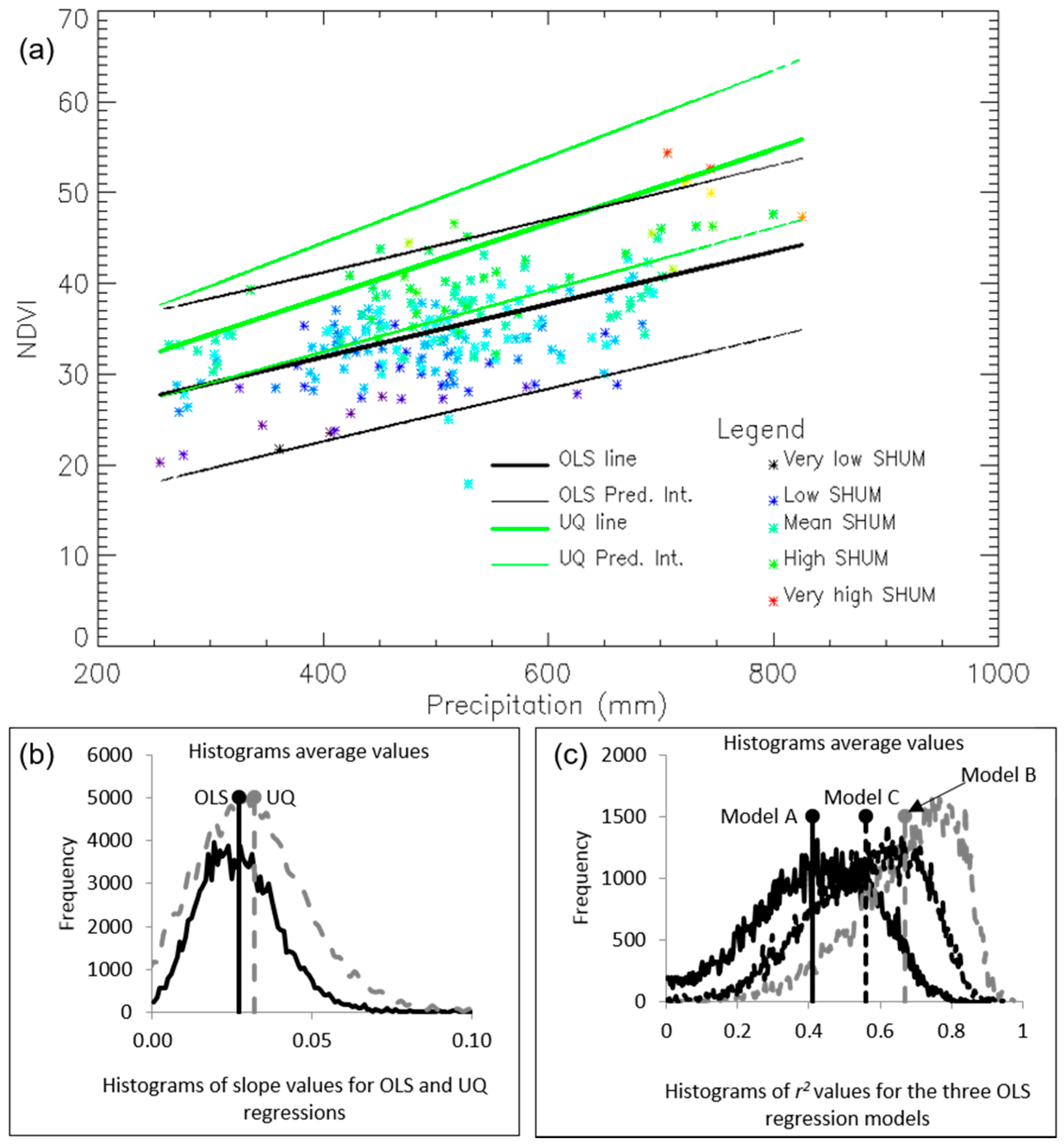
The analyses clearly indicated that variance in ΣNDVI_gs (the surrogate for NPP) was better explained by combined growing season precipitation, specific humidity, and temperature, and by seasonal variance and skewness of precipitation, rather than by RUE (precipitation alone-Model A) (Figure 2d). This was expected because of the roles these meteorological variables play in growth and rates of development of vegetation throughout the Sahel [37,85,86,87]. However, it should be recognized that herbaceous and woody components of the vegetation, which may vary independently [88], were not distinguished here.

The proportion of significant relationships between precipitation and ΣNDVI_gs found here was similar to other reports [89]—the differences probably related to the different preprocessing of data used and inclusion or exclusion of precipitation outside the main growing season, although there is another study [28] that reported a very low percentage of the region with significant relationships.

Despite significant increases in r² values, the strength of the relationship between ΣNDVI_gs and the meteorological variables was not uniformly high. For example, it was relatively weak south of the 900mm isohyet (Figure 3), presumably because the environmental variables studied do not limit NPP there to the same degree as in the drier areas [37,88]. In drier areas, low correlations may arise near perennial lakes, rivers, and irrigated agriculture where the vegetation can utilize water from rainfall gathered elsewhere (in which case precondition (iii) for RUE would not be met (Table 1). Similarly, for trees which may access water deep in the soil profile [90] (also not satisfying precondition (iii). Table 1), or, in some cases, the rainfall–soil moisture relationship can become increasingly non-linear (not satisfying precondition (i)) owing to reduced infiltration and surface evaporation.

Potential ΣNDVI_gs prediction errors were calculated with the assumption that the meteorological datasets were error-free. This is clearly not the case and could reduce the extent of the areas with significant trends. Unfortunately, modeled meteorological data sets are rarely accompanied by measures of error, and tests with meteorological stations data are not valid since those data are used in calibration [49]. Moreover, the systematic error component of the AVHRR data has not been evaluated, since data from other sensors were not available for the full study period (1982–2006). However, the corrections applied to the meteorological and to the AVHRR data [49,57] have been applied to the processing stream and are reported to significantly reduce the systematic error components and therefore are not expected to have influenced greatly the findings of this study.

Potential ΣNDVI_gs values estimated from OLS regressions were generally lower than their counterparts obtained from the 95^th upper quantile (UQ) distribution (Figure 1). This was expected, since OLS regressions can underestimate vegetation production potential because, in years when vegetation production was not only limited by precipitation, other factors, including humidity and temperature, in addition to degradation, can reduce the estimate of potential production [32]. Furthermore, a number of slow processes, such as depletion of seed and bud banks [91], nutrient limitations, excessive run-off, grazing, and fuel-wood collection [92] among other causes, may also contribute, and result in an under estimation of potential vegetation production [32]. Sites affected by these are indistinguishable from those at their potential (so precondition (vi) for use of RUE is not met (Table 1)) and the mean rates of change in ΣNDVI_gs would underestimate the production expected in response to climate variability (i.e., potential ΣNDVI_gs values), reducing the “degradation” signal and overestimating the “greening” signal. This is not to suggest that estimating potential ΣNDVI_gs using UQ regression functions is without its own problems; it is still subject to the same errors as OLS because it is also affected by the degraded sites, albeit using a more appropriate statistical model.

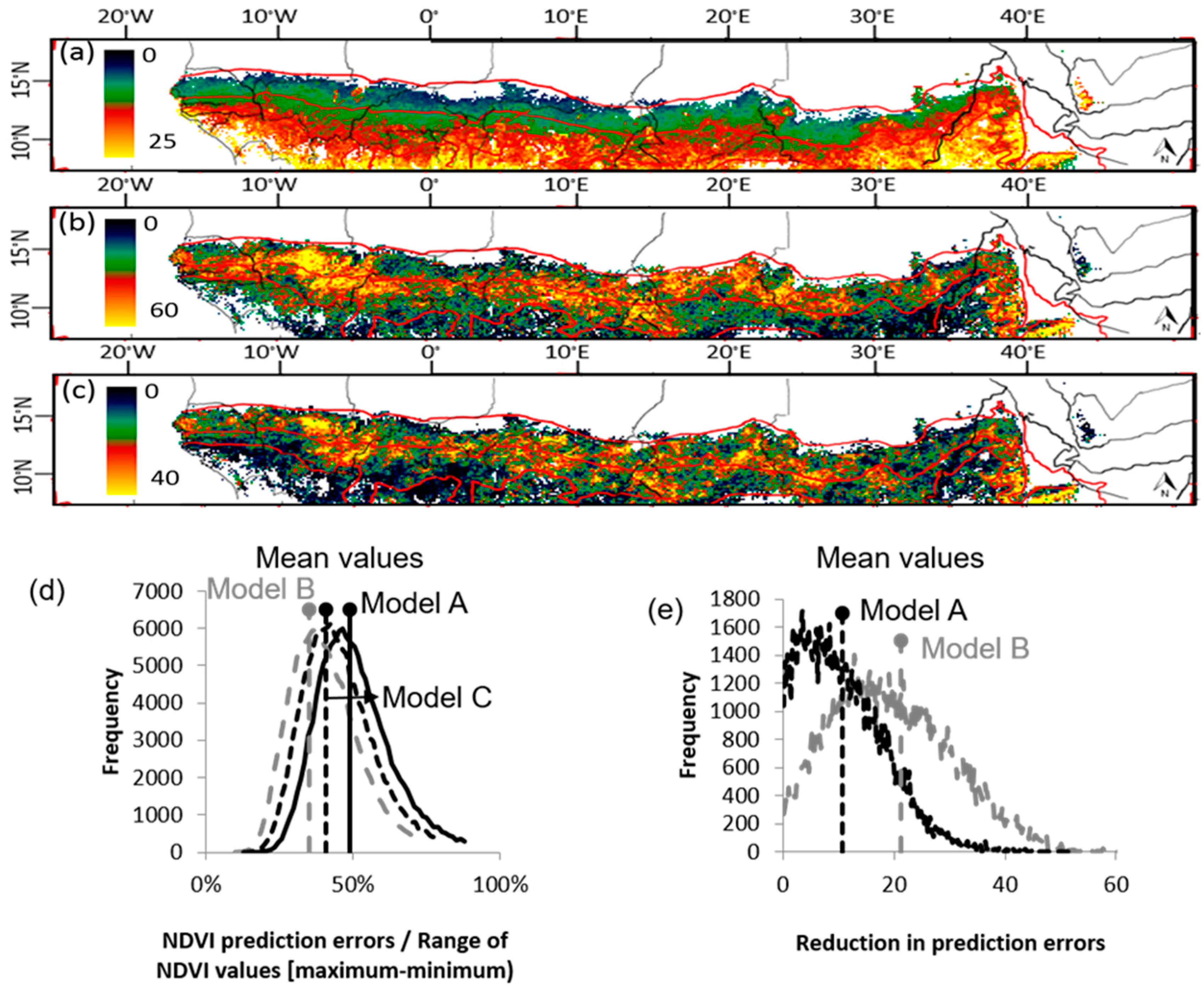
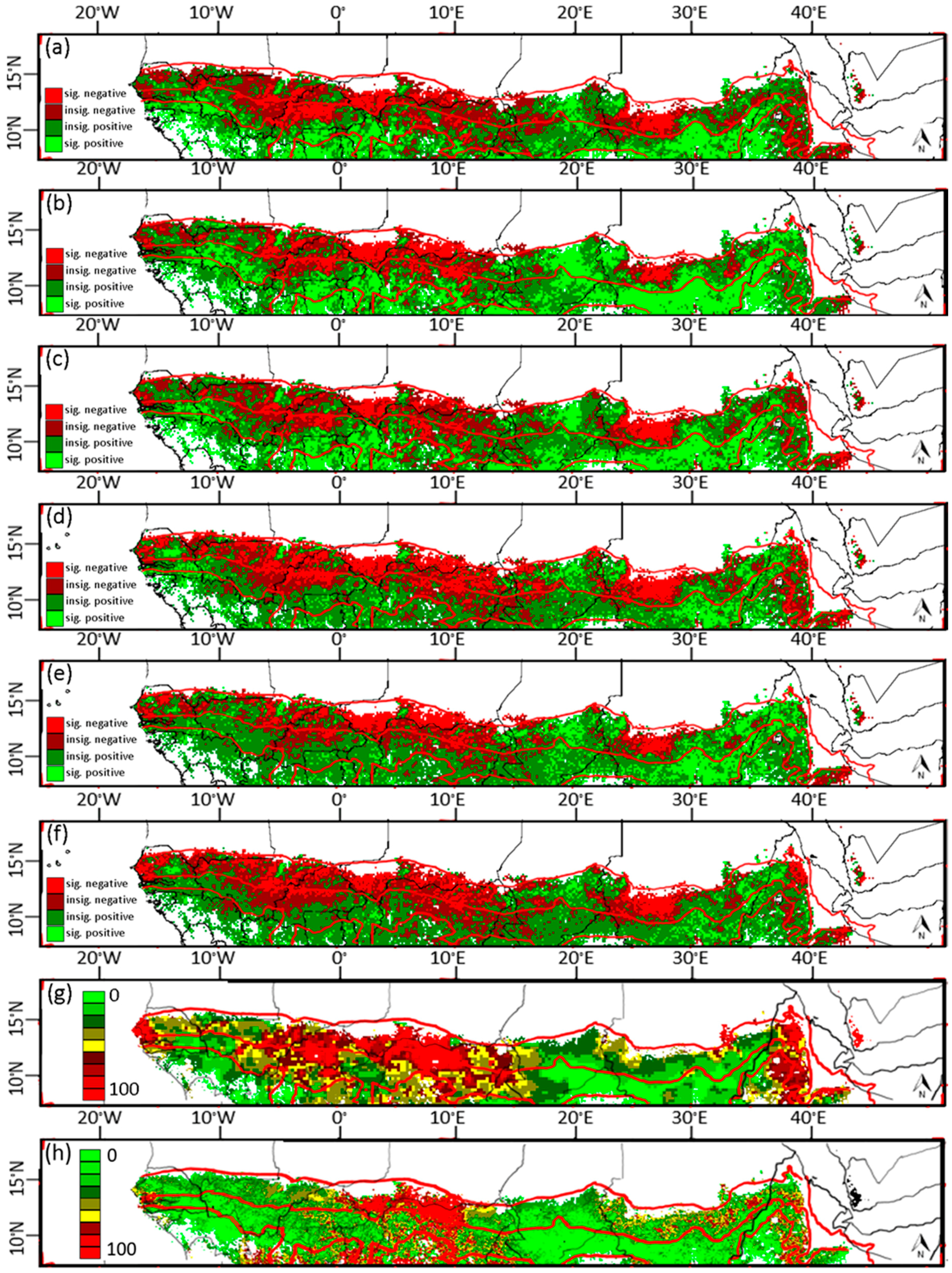
The OLS RESTREND models (models A, B, and C) resulted in larger areas with significant positive trends than the UQ based RESTREND models (models D, E, and F) (

Table 6. Percentage land area with significant negative and positive trends. OLS—ordinary least squares; UQ—upper quartile regression.

RESTREND Regression Models	Model Independent Variables	Significant Negative Trends	Insignificant Negative Trends	Significant Positive Trends	Insignificant Positive Trends
A (OLS)	precipitation	7.22%	28.72%	25.29%	38.78%
D (UQ)		12.88%	27.22%	12.73%	47.18%
B (OLS)	precipitation, specific humidity, and temperature	7.14%	18.86%	34.20%	39.80%
E (UQ)		8.01%	20.93%	16.84%	54.22%
C (OLS)	precipitation, variance, and skewness of intra-annual precipitation frequency	6.60%	25.40%	25.59%	42.41%
F (UQ)		9.85%	30.77%	7.25%	52.12%

), however, in all cases the largest areas had no significant trends (mean of all models 70%), in agreement with other studies (e.g., [28,101]). Despite the differences between the models in the significance of these trends, they all indicate large and spatially coherent areas that “greened” faster than can be accounted for by changes in meteorological conditions (Figure 4) [88,102]. Similarly, after removing the effects of rainfall on NDVI, positive trends have been found, for example, over parts of the Senegal, Southern Mali, and Chad and the entire Sahel [28,30,88,103,104,105]. Explanations of the greening trends in the literature include agricultural intensification, improvements in soil and water conservation techniques, supplementary irrigation, and fertilization, all as a result of increased investment [88], CO₂ fertilization, increased carry-over effects of soil moisture from previous wet years, and increases in seed and bud banks associated with high vegetation productivity in previous years [32,90,102,105,106,107,108]. The present results also detected large parts of Burkina Faso, northern Nigeria, southern Niger, and western Sudan with significant negative trends (Figure 4). Surprisingly, similar analyses (e.g., [105]) have not found this pattern, possibly because different data sets were used. In addition to the frequently quoted effects of excessive cultivation, increases in grazing, etc., suggestions for the negative trends include land abandonment associated with economic migration and civil strife, and transitions to new quasi-stable vegetation composition following the extreme droughts of the 1970s and 1980s [20,27,32,33,43]. Even though some disagreement can be expected due to differences between the climate datasets used here and in other studies, and because of differences in the AVHRR data used [105], the lack of agreement over such large areas is surprising.

The RESTREND results were compared qualitatively with published case studies of land degradation and rehabilitation in the Sahel ([12,30,97,98,100,101,102,103,104,105,106,107,108,109,110]) and by comparison with field observations by experts (e.g., Gray Tappan, 2008 pers. com.). While these comparisons showed favorable agreement (

Table 7. Comparisons between RESTREND results and published literature on the status of land degradation and land use in the Sahel.

Geographical Region & Period Studied	Degradation Symptoms	Pressures	Opportunities	Sources	Residual Trends (RESTREND) Comparisons
Maradi (southern Niger) and Kano (northern Nigeria) Departments (1960–2000)	Soil fertility decline, soil erosion	Grazing, cultivation without fertilization of outlying fields, loss of woody vegetation cover, aridity	Greater use of manure and mineral fertilizers (1990–2000)	[93,94]	All models show significant negative residual trends
	Vegetation degradation	Intensified grazing pressure, aridity, deforestation, agricultural expansion	Stable or increasing densities of trees being maintained on farmland; but natural woodlands still under pressure	[95,96,97]
	Loss of agricultural productivity	Collapse of the long fallowing system	Increased livestock production through transhumance and increased use of crop residue	[95,97]
Diourbel Region (Senegal) (1960–2000)	Drop in groundnut yields/mm rainfall. Millet yields/mm rainfall stable (1982–1998)	Shortening of the fallow period, insufficient application of manure, high prices of inputs (e.g., mineral fertilizers)	No data	[98]	OLS models (insignificant negative trends); UQ based models (significant negative trends)
	Vegetation degradation. Woody cover declined from 7.7% in 1978 to 2.8% in 1989	Fuelwood and construction timber collection, aridity, farm expansion	Increasing densities of trees being maintained on farmland	[99]
	Decline in soil fertility	Shortening of fallow cycle, reduction in mineral fertilization post 1980	Increasing manure application from the buoyant livestock sector	[98]
Senegal (Ferlo region)	Decline in woody cover but mainly attributed to drought	Expansion of agriculture into climatically marginal regions), encouraged by national policy (maintaining land in production); % cropland area reached 16% by 2000.	No data	[100]	Large areas of the Ferlo have negative trends though insignificant in most models.
Senegal (ferruginous pastoral ecoregion)	High rates of woody cover mortality; expansion on barren land from 0.3% in 1965 to 4.5% in 1999	Aridity, overgrazing, soil compaction	No data	[100]	Negative–significant negative trends in the eastern parts of the region; positive insignificant trends in western parts
Senegal (West central agricultural ecoregion, or Peanut Basin)	No data	Post 1985 abandonment of agricultural land (%area dropped from 80% to 67% in 2000)	No data	[100]	Positive but insignificant trends in the northern part; negative but insignificant trends in the southern part.
Senegal (Eastern transition zone)	No data	Half of the wooded savannas has been degraded by charcoal production (post 1985). Bushfires, agricultural expansion (4% of the total area) and grazing are secondary pressures	No data	[100]	Northeastern area with negative–significantly negative trends; remaining area have positive but insignificant
Senegal (Agricultural expansion region and Saloum agricultural	Deforestation and degradation inferred from analysis of aerial photos	Conversion of wooded savannas and forests into agriculture (almost the entire area was transformed)	No data	[100]	Negative–significant negative trends. Lower values were obtained for the Saloum region.
Shield ecoregion (South -east Senegal)	No data	Agriculture (only 2% of the landscape) with long fallow periods still practiced	No data	[100]	Significant positive trends
Senegal—Casamance (Sudano—Guinean zone in South)	No data	Post 1985 rapid agricultural expansion in the middle eastern part of the region, coupled with fuel wood extraction	No data	[100]	Positive–significantly positive trends in the eastern and western parts. Negative but insignificant trends in in the middle parts of the region
Sahel region	Coordinates of degraded/non-degraded landscapes throughout the Sahel.	No data	No data	Tappan, G. pers. comm.	Good agreement (>70%) with model results

), they should not be construed as validation results. Validation sensu stricto requires direct measurements of vegetation at appropriate scales over a distributed set of sites. Until such datasets become available, validation of satellite-derived degradation indices at the scales studied here will not be easy.

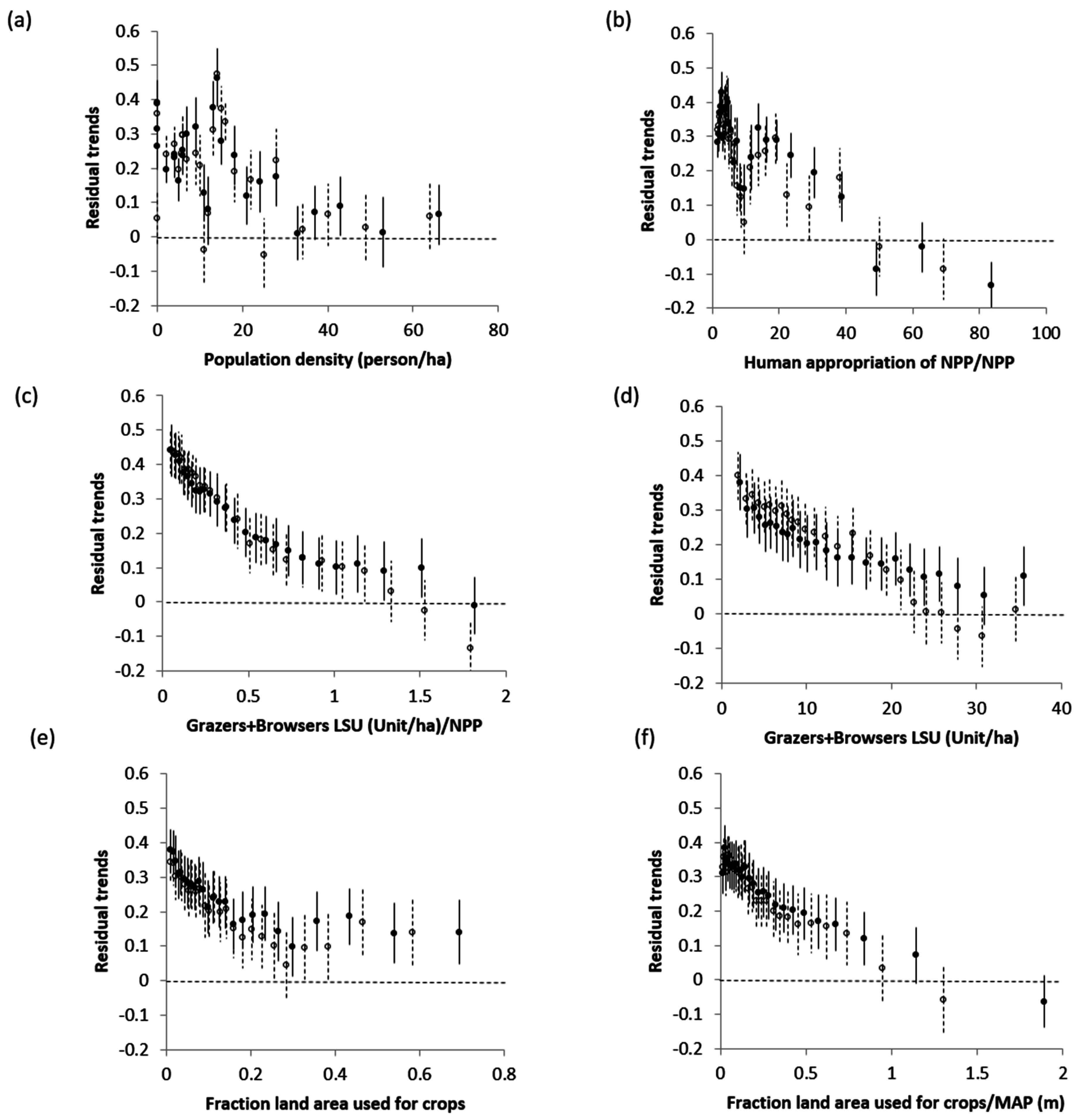
Analysis of the relation between RESTREND values and population density did not support the notion that higher population density in the Sahel invariably causes reductions in land productivity (Table 4 and Table 5). %HANPP, on the other hand, was related to reductions in land productivity (r = −0.55). It should be noted that the calculation of %HANPP [66] does not account for lateral flows (imports or exports) of NPP-based products. Including these effects may provide a better accounting of the pressures people impose on their local environment. Nevertheless, the relationship between %HANPP and RESTREND was strong enough to suggest that higher demands for NPP-based goods in relation to local NPP production are likely to impoverish local ecosystems [111].

Further examination of the relation of land uses such as livestock production and area of land used in cultivation with the RESTREND values found moderate–weak correlations (Table 4). However, stronger relationships were found between RESTREND and the ratios of both LSU to livestock carrying capacity (LSU/NPP; r = −0.51) and %crop area to mean annual precipitation (%crop/MAP; r = −0.55). While the inverse relationship between RESTREND values and LSU/NPP was expected, the relation with %crop/MAP suggests that the extension of cultivation into marginal lands, not suitable for agriculture, may result in long-term reductions in productivity or degradation [15,80].

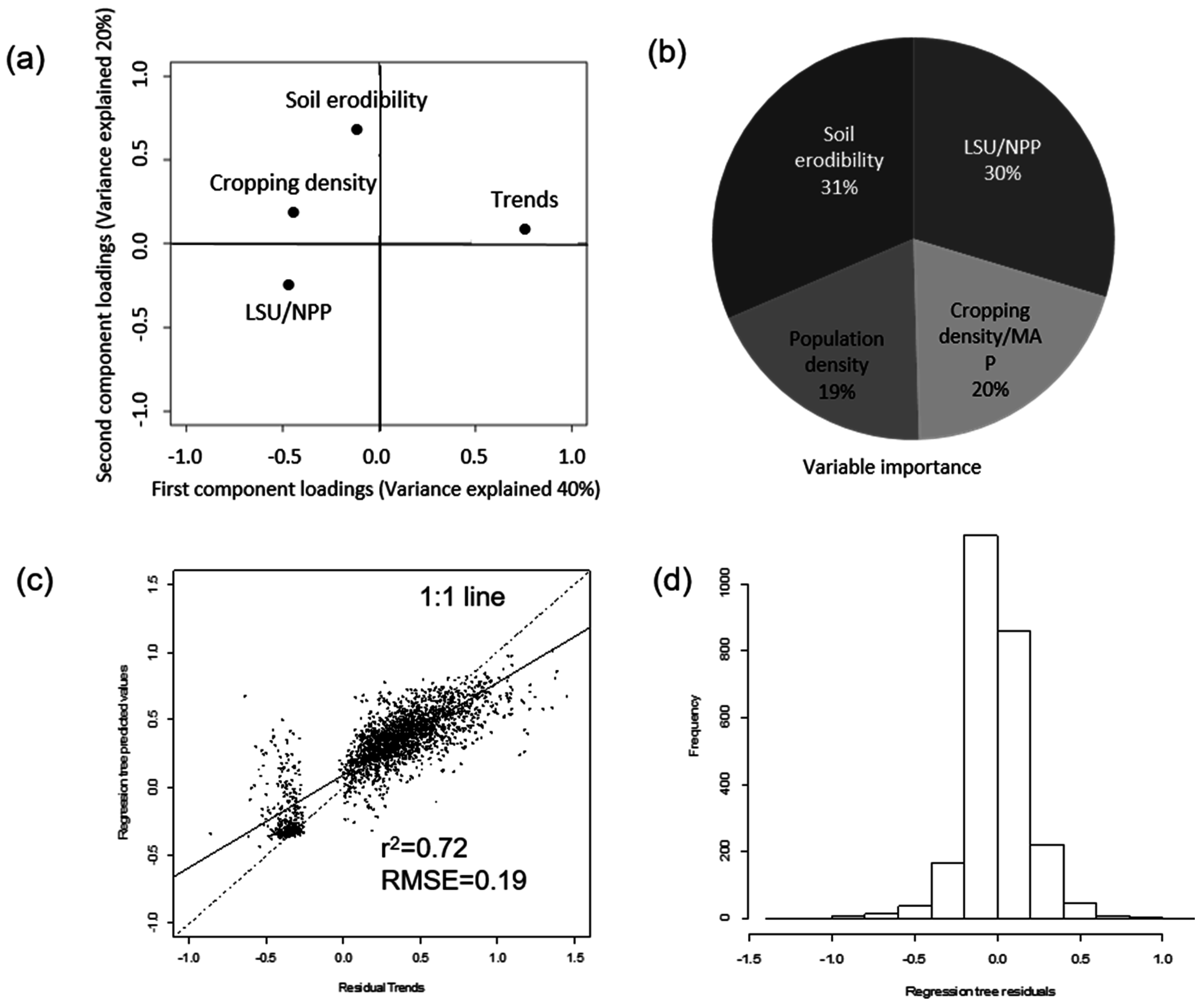
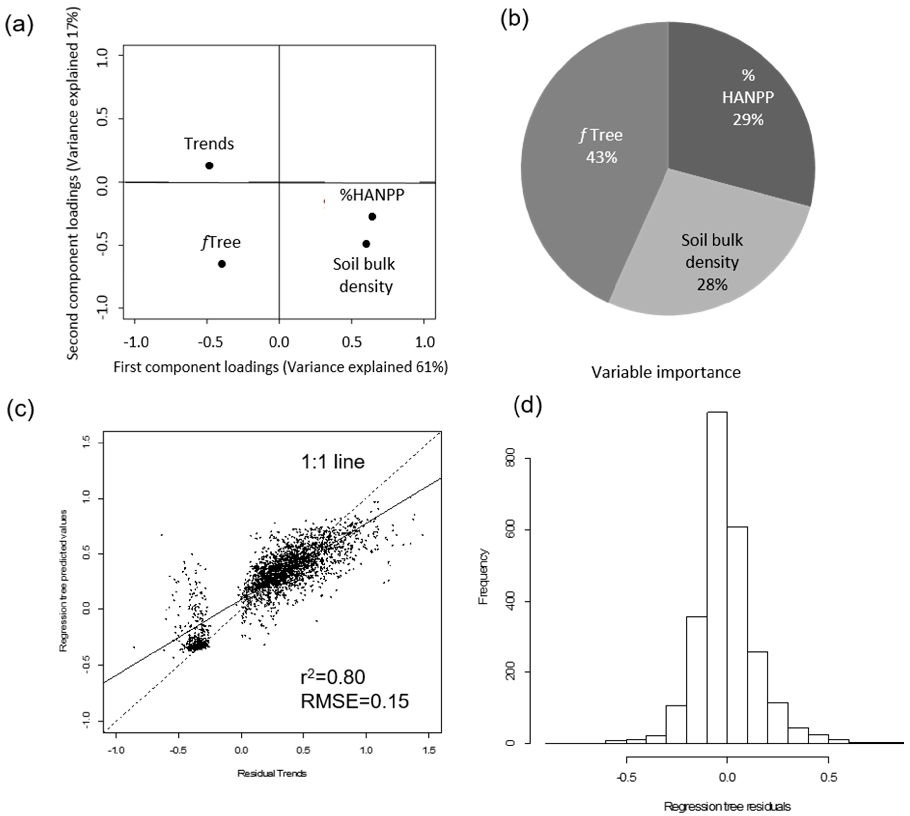
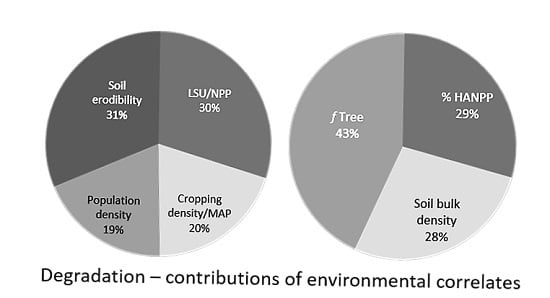
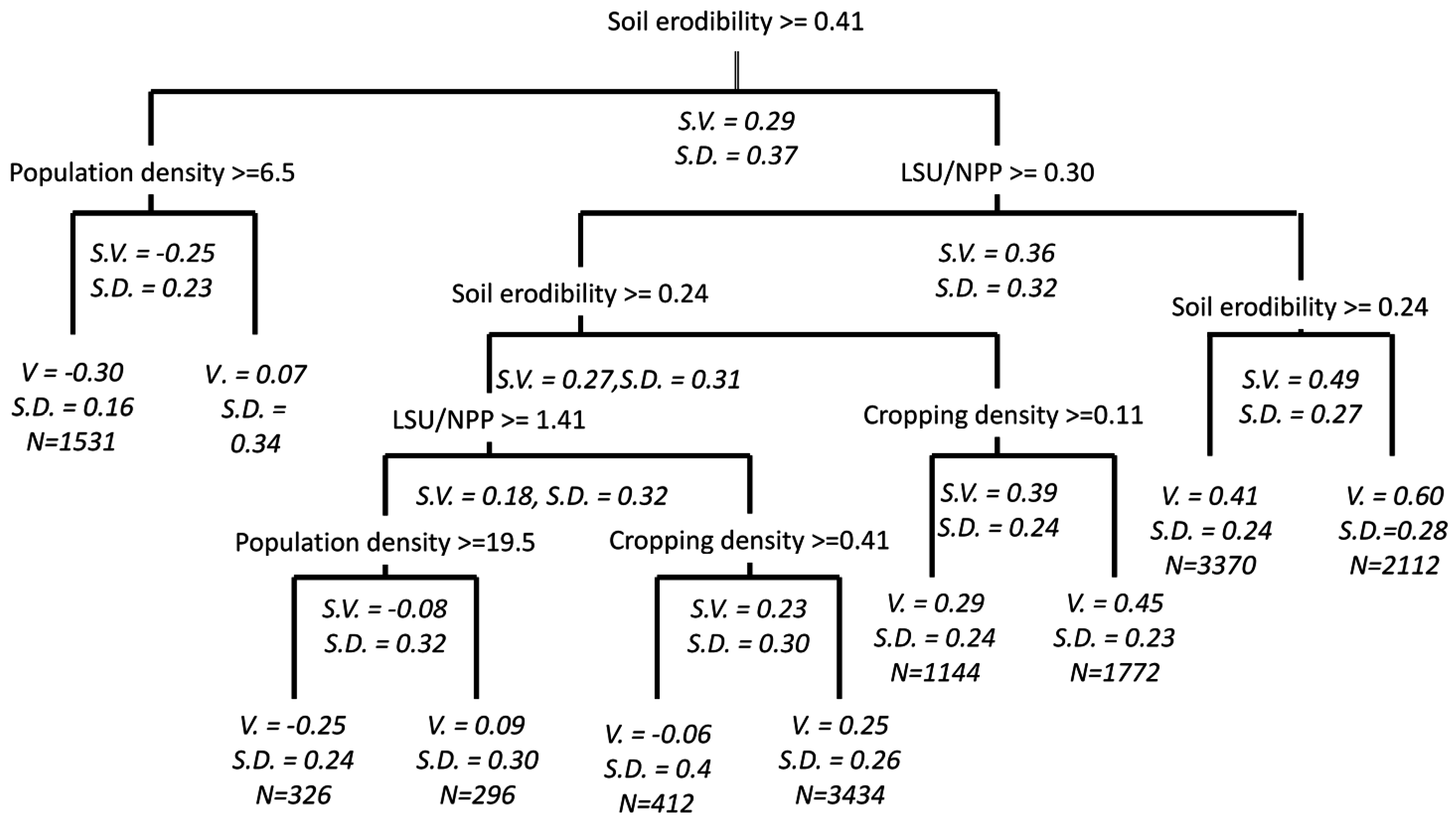
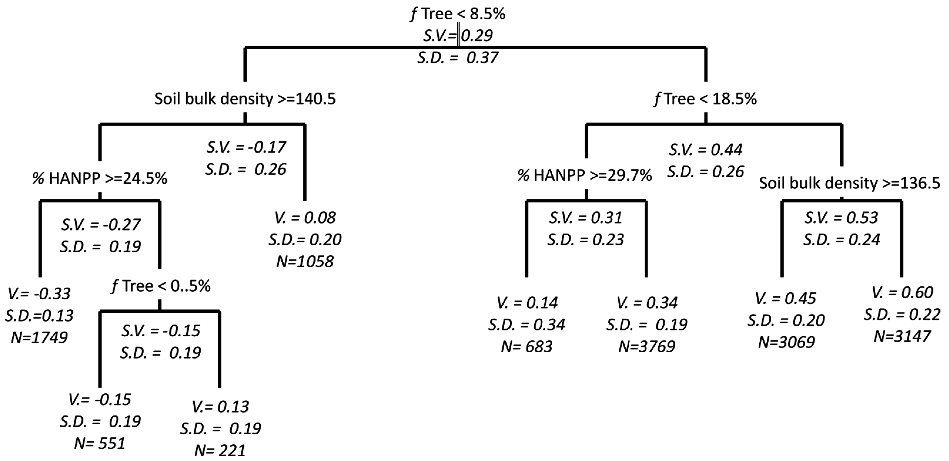
A meta-analysis of case studies of land degradation [80] found that, contrary to the theory of single-factor causation [53,112], land degradation in Africa can more often be attributed to multiple factors, and even to remote influences, including changes in agricultural policies such as intensification of livestock production, production of cash crops, and irrigation. Also, the spatial variations in RESTREND values were not only better explained by a multiplicity of land uses but also by local variations in natural resource endowments (Figure 6 and Figure 7). Of the biophysical variables explored, soil bulk density, soil erodibility, and the fraction land area covered by trees were strongly related to degradation of NPP. These variables also enhanced the adverse effects of population and land use pressures (Figure 8 and Figure 9). One possible mechanism is that fuel wood collection, agriculture, and grazing reduce perennial plant cover and simplify the vegetation structure exposing the soil to wind and water erosion [15]; also soil erosion and dispersion rates are higher in landscapes with higher soil bulk density and soil erodibility [113,114,115,116].

5. Conclusions

Many studies have demonstrated that the return of more favorable climate conditions in the Sahel following the extreme droughts of the 1970s and early 1980s has been accompanied by a net increase in vegetation greenness (e.g., [26,102,103,117]). Yet, the spatial variations in the rates of vegetation recovery can only partially be explained by climate trends [27,88,118], thus reinvigorating the debate about the influence of anthropogenic land degradation and restoration on vegetation productivity [22,23]. The focus of this study was therefore twofold: first, to investigate where the land surface in the Sahel has been greening “faster” (i.e., positive RESTREND), or “slower” (i.e., negative RESTREND) than what would be expected from the trends in climate; and, second, to relate the spatial variations in RESTREND values to land use and human population density.

The results suggest that, over large areas of the Sahel, the average area of insignificant trends was 70%, similar or larger than reported in other studies (e.g., [88]). Overall, in >87% of the area, NPP (vegetation greenness) either exceeded (i.e., positive RESTREND) or did not significantly depart from what is expected from the trends in climate (i.e., insignificant RESTREND). The areas with positive RESTREND were frequently associated with relatively low population and land use pressures. Undoubtedly, there are places where land rehabilitation efforts have increased land productivity—perhaps irrigation, shortened fallow period, erosion control, fertilizer use, CO₂ fertilization (e.g., [20])—but, at the scale of observation used here, there was little evidence to suggest that land rehabilitation or agricultural intensification were adequate explanations of the long-term increases in NPP. The scales of the phenomena and the explanations must match; explanations that do include an increase in water use efficiency caused by CO₂ fertilization, higher nitrogen deposition, higher atmospheric aerosol loadings, or transitions to new quasi-stable vegetation compositions following the extreme droughts of the 1970s and 1980s [43,119,120,121,122] and, perhaps, non-linear, accelerating responses of vegetation to the changing climate, do fit the scale of the satellite observations.

Contrary to findings in similar studies [28,30], we found large (7%–13% of the study area), spatially coherent areas with significant negative trends in production. These areas were found to have high livestock densities relative to their carrying capacity, intensive cultivation, overworked marginal lands, or combinations of these. The results suggest that population and land use pressures have had a measurable impact on vegetation dynamics in some parts of the Sahel during the period 1982–2006.

References

1. United Nations. World Population Prospects the 2010 Revision Volume I: Comprehensive Tables; Department of Economic and Social Affairs, Population Division: New York, NY, USA, 2011; [CD-ROM]. [Google Scholar]
2. Lambin, E.F.; Geist, H.J.; Lepers, E. Dynamics of land-use and land-cover change in tropical regions. Ann. Rev. Environ. Resour. 2003, 28, 205–241. [Google Scholar] [CrossRef]
3. Ramaswamy, S.; Sanders, J.H. Population pressure, land degradation and sustainable agricultural technologies in the Sahel. Agric. Syst. 1992, 40, 361–378. [Google Scholar] [CrossRef]
4. Vierich, H.I.D.; Stoop, W.A. Changes in West African savanna agriculture in response to growing population and continuing low rainfall. Agric. Ecosyst. Environ. 1990, 31, 115–132. [Google Scholar] [CrossRef]
5. Food and Agriculture Organization of the United Nations (FAOSTAT). Livestock Primary Statistical Database; FAOSTAT: Rome, Italy, 2011. [Google Scholar]
6. Van de Koppel, J.; Rietkerk, M.; Weissing, F.J. Catastrophic vegetation shifts and soil degradation in terrestrial grazing systems. Trends Ecol. Evolut. 1997, 12, 352–356. [Google Scholar] [CrossRef]
7. Le Barbé, L.; Lebel, T.; Tapsoba, D. Rainfall variability in West Africa during the years 1950–90. J. Clim. 2002, 15, 187–202. [Google Scholar] [CrossRef]
8. Nicholson, S.E. Climatic and environmental change in Africa during the last two centuries. Clim. Res. 2001, 17, 123–144. [Google Scholar] [CrossRef]
9. Tucker, C.J.; Dregne, H.E.; Newcomb, W.W. Expansion and contraction of the Sahara Desert from 1980 to 1990. Science 1991, 253, 299–301. [Google Scholar] [CrossRef] [PubMed]
10. Venema, H.D.; Schiller, E.J.; Adamowski, K.; Thizy, J.M. A water resources planning response to climate change in the Senegal River basin. J. Environ. Manag. 1997, 49, 125–155. [Google Scholar] [CrossRef]
11. Senjobi, B.A.; Ogunkunle, O.A. Effect of land use on soil degradation and soil productivity decline on alfisols and ultisols in Ogun state in south western Nigeria. Agric. Conspec. Sci. 2010, 75, 9–19. [Google Scholar]
12. Hurni, H.; Tato, K.; Zeleke, G. The implications of changes in population, land use, and land management for surface runoff in the upper Nile basin area of Ethiopia. Mt. Res. Dev. 2005, 25, 147–154. [Google Scholar] [CrossRef]
13. Norman, C. Expanding deserts, shrinking resources. Science 1987, 235. [Google Scholar] [CrossRef] [PubMed]
14. Lamprey, H. Report on the desert encroachment reconnaissance in northern Sudan: 21 October to 10 November 1975. Desertification Control Bull. 1988, 17, 1–7. [Google Scholar]
15. Le Houérou, H.N. Climate change, drought and desertification. J. Arid Environ. 1996, 34, 133–185. [Google Scholar] [CrossRef]
16. Mazzucato, V.; Niemeijer, D. Rethinking Soil and Water Conservation in a Changing Society: A Case Study in Eastern Burkina Faso; Wageningen University: Wageningen, The Netherlands, 2000; p. 409. [Google Scholar]
17. Tiffen, M.; Mortimore, M.; Gichuki, F. More People, Less Erosion, Kenyan ed.; ACTS Press: Nairobi, Kenya, 1994. [Google Scholar]
18. Adams, W.M.; Mortimore, M.J. Agricultural intensification and flexibility in the Nigerian Sahel. Geogr. J. 1997, 163, 150–160. [Google Scholar] [CrossRef]
19. Mortimore, M.; Harris, F. Do small farmers’ achievements contradict the nutrient depletion scenarios for Africa? Land Use Policy 2005, 22, 43–56. [Google Scholar] [CrossRef]
20. Mortimore, M.; Turner, B. Does the Sahelian smallholder’s management of woodland, farm trees, rangeland support the hypothesis of human-induced desertification? J. Arid Environ. 2005, 63, 567–595. [Google Scholar] [CrossRef]
21. Rasmussen, K.; D’Haen, S.; Fensholt, R.; Fog, B.; Horion, S.; Nielsen, J.O.; Rasmussen, L.V.; Reenberg, A. Environmental change in the Sahel: Reconciling contrasting evidence and interpretations. Reg. Environ. Chang. 2016, 16, 673–680. [Google Scholar] [CrossRef]
22. Hein, L.; de Ridder, N.; Hiernaux, P.; Leemans, R.; de Wit, A.; Schaepman, M. Desertification in the Sahel: Towards better accounting for ecosystem dynamics in the interpretation of remote sensing images. J. Arid Environ. 2011, 75, 1164–1172. [Google Scholar] [CrossRef]
23. Hein, L.; De Ridder, N. Desertification in the Sahel: A reinterpretation. Glob. Chang. Biol. 2006, 12, 751–758. [Google Scholar] [CrossRef]
24. Prince, S.D.; Wessels, K.J.; Tucker, C.J.; Nicholson, S.E. Desertification in the Sahel: A reinterpretation of a reinterpretation. Glob. Chang. Biol. 2007, 13, 1308–1313. [Google Scholar] [CrossRef]
25. Behnke, R.; Mortimore, M. The End of Desertification? Disputing Environmental Change in Drylands; Springer Earth System Science Series: Berlin/Heidelberg, Germany, 2016. [Google Scholar]
26. Eklundh, L.; Olsson, L. Vegetation index trends for the African Sahel 1982–1999. Geophys. Res. Lett. 2003, 30. [Google Scholar] [CrossRef]
27. Olsson, L.; Eklundh, L.; Ardö, J. A recent greening of the Sahel-trends, patterns and potential causes. J. Arid Environ. 2005, 63, 556–566. [Google Scholar] [CrossRef]
28. Fensholt, R.; Rasmussen, K. Analysis of trends in the Sahelian ‘rain-use efficiency’ using GIMMS NDVI, RFE and GPCP rainfall data. Remote Sens. Environ. 2011, 115, 438–451. [Google Scholar] [CrossRef]
29. Tucker, C.J.; Nicholson, S.E. Variations in the size of the Sahara Desert from 1980 to 1997. Ambio 1999, 28, 587–591. [Google Scholar]
30. Herrmann, S.M.; Anyamba, A.; Tucker, C.J. Recent trends in vegetation dynamics in the African Sahel and their relationship to climate. Glob. Environ. Chang. A 2005, 15, 394–404. [Google Scholar] [CrossRef]
31. Heumann, B.W.; Seaquist, J.W.; Eklundh, L.; Jonsson, P. AVHRR derived phenological change in the Sahel and Soudan, Africa, 1982–2005. Remote Sens. Environ. 2007, 108, 385–392. [Google Scholar] [CrossRef]
32. Prince, S.D.; De Colstoun, E.B.; Kravitz, L.L. Evidence from rain-use efficiencies does not indicate extensive Sahelian desertification. Glob. Chang. Biol. 1998, 4, 359–374. [Google Scholar] [CrossRef]
33. Prince, S.D. Spatial and temporal scales for detection of desertification. In Global Desertification: Do Humans Cause Deserts; Reynolds, J., Stafford Smith, D., Eds.; Dahlem University Press: Berlin, Germany, 2002; pp. 23–40. [Google Scholar]
34. Safriel, U. The assessment of global trends in land degradation. Clim. Land Degrad. 2007, 1–38. [Google Scholar]
35. Nicholson, S.E. Desertification. In Dryland Climatology; Nicholson, S.E., Ed.; Cambridge University Press: New York, NY, USA, 2011; pp. 431–447. [Google Scholar]
36. Wessels, K.J.; Prince, S.D.; Malherbe, J.; Small, J.; Frost, P.E.; VanZyl, D. Can human-induced land degradation be distinguished from the effects of rainfall variability? A case study in South Africa. J. Arid Environ. 2007, 68, 271–297. [Google Scholar] [CrossRef]
37. Rishmawi, K.N.; Prince, S.D.; Xue, Y. Vegetation responses to climate variability in the northern arid to sub-humid zones of Sub-Saharan Africa. Remote Sens. 2016, 8, 910. [Google Scholar] [CrossRef]
38. Evans, J.; Geerken, R. Discrimination between climate and human-induced dryland degradation. J. Arid Environ. 2004, 57, 535–554. [Google Scholar] [CrossRef]
39. Jackson, H.; Prince, S.D. Degradation of net primary production in a semiarid rangeland. Biogeosciences 2016, 13, 4721–4734. [Google Scholar] [CrossRef]
40. Jackson, H.; Prince, S.D. Degradation of non-photosynthetic vegetation in a semi-arid rangeland. Remote Sens. 2016, 8, 692. [Google Scholar] [CrossRef]
41. Prince, S.D. Where does desertification occur? Mapping dryland degradation at regional to global scales. In The End of Desertification? Disputing Environmental Change in Drylands; Behnke, R., Mortimore, M., Eds.; Springer: Heidelberg, Germany, 2016; pp. 225–263. [Google Scholar]
42. Running, S.W.; Hunt, E.R.J. Generalization of a forest ecosystem process model for other biomes, BIOME-BGC and an application for global-scale models. In Scaling Physiological Processes: Leaf to Globe; Ehleringer, J.R., Field, C.B., Eds.; Academic Press: San Diego, CA, USA, 1993; pp. 141–158. [Google Scholar]
43. Hickler, T.; Eklundh, L.; Seaquist, J.W.; Smith, B.; Ardö, J.; Olsson, L.; Sykes, M.; Sjöström, M. Precipitation controls Sahel greening trend. Geophys. Res. Lett. 2005, 32. [Google Scholar] [CrossRef]
44. Jetten, V.; de Roo, A.; Favis-Mortlock, D. Evaluation of field-scale and catchment-scale soil erosion models. CATENA 1999, 37, 521–541. [Google Scholar] [CrossRef]
45. Bai, Z.G.; Dent, D.L.; Olsson, L.; Schaepman, M.E. Proxy global assessment of land degradation. Soil Use Manag. 2008, 24, 223–234. [Google Scholar] [CrossRef]
46. Koenker, R. Quantile Regression (Econometric Society Monographs, Series 38); Cambridge University Press: Cambridge, UK, 2005. [Google Scholar]
47. Koenker, R.; Hallock, K.F. Quantile regression. J. Econ. Perspect. 2001, 15, 143–156. [Google Scholar] [CrossRef]
48. Koenker, R.; Bassett, G., Jr. Regression quantiles. Econometrica 1978, 46, 33–50. [Google Scholar] [CrossRef]
49. Sheffield, J.; Goteti, G.; Wood, E.F. Development of a 50-year high-resolution global dataset of meteorological forcings for land surface modeling. J. Clim. 2006, 19, 3088–3111. [Google Scholar] [CrossRef]
50. Wessels, K.J.; Prince, S.D.; Malherbe, J.; Small, J.; Frost, P.E.; VanZyl, D. Can human-induced land degradation be distinguished from the effects of rainfall variability? A case study in South Africa. J. Arid Environ. 2007, 68, 271–297. [Google Scholar] [CrossRef]
51. Scott, E.P. Land use change in the harsh lands of West Africa. Afr. Stud. Rev. 1979, 22, 1–24. [Google Scholar] [CrossRef]
52. Cleaver, K.M.; Schreiber, G.A. Reversing the Spiral: The Population, Agriculture, and Environmental Nexus in Sub-Saharan Africa; The World Bank: Washington, D.C., USA, 1994. [Google Scholar]
53. Le Houérou, H.N. Man-made deserts: Desertization processes and threats. Arid Land Res. Manag. 2002, 16, 1–36. [Google Scholar] [CrossRef]
54. Lal, R.; Wagner, A.; Greenland, D.J.; Quine, T.; Billing, D.W.; Evans, R.; Giller, K. Degradation and resilience of soils [and discussion]. Philos. Trans. Biol. Sci. 1997, 352, 997–1010. [Google Scholar] [CrossRef]
55. Pedelty, J.; Devadiga, S.; Masuoka, E.; Brown, M.; Pinzon, J.; Roy, D.; Vermote, E.; Prince, S.; Nagol, J.; Justice, C.; et al. Generating a long-term land data record from the AVHRR and MODIS instruments. In Proceedings of the International Geoscience and Remote Sensing Symposium, Barcelona, Spain, 23–28 July 2007.
56. Rishmawi, K.N. Spatial Patterns and Potential Mechanisms of Land Degradation in the Sahel. Ph.D. Thesis, University of Maryland, College Park, MD, USA, 2013. [Google Scholar]
57. Nagol, J.R.; Vermote, E.F.; Prince, S.D. Effects of atmospheric variation on AVHRR NDVI data. Remote Sens. Environ. 2009, 113, 392–397. [Google Scholar] [CrossRef]
58. Center for International Earth Science Information Network (CIESIN). Gridded Population of the World Population Density Grid, version 3 (GPWV3); Socioeconomic Data and Applications Center (SEDAC), Columbia University: New York, NY, USA; United Nations Food and Agriculture Programme (FAO): New York, NY, USA; Centro Internacional De Agricultura Tropical (CIAT): Palisades, NY, USA, 2005; Available online: http://sedac.Ciesin.Columbia.Edu/gpw (accessed on 1 July 2011).
59. Ramankutty, N.; Evan, A.T.; Monfreda, C.; Foley, J.A. Farming the planet: 1. Geographic distribution of global agricultural lands in the year 2000. Glob. Biogeochem. Cycles 2008, 22. [Google Scholar] [CrossRef]
60. Robinson, T.P.; Franceschini, G.; Wint, W. The food and agriculture organization’s gridded livestock of the world. Vet. Ital. 2007, 43, 745–751. [Google Scholar] [PubMed]
61. Jahnke, H.E. Livestock Production Systems and Livestock Development in Tropical Africa; Kieler Wissenschaftsverlag Vauk: Kiel, Germany, 1982. [Google Scholar]
62. Wilson, A.; Leigh, J.; Hindley, N.; Mulham, W. Comparison of the diets of goats and sheep on a Casuarina cristata-Heterodendrum oleifolium woodland community in western New South Wales. Aust. J. Exp. Agric. Anim. Husb. 1975, 15, 45–53. [Google Scholar] [CrossRef]
63. Pfister, J.A.; Malechek, J.C. The voluntary forage intake and nutrition of goats and sheep in the semi-arid tropics of northeastern Brazil. J. Anim. Sci. 1986, 63, 1078–1086. [Google Scholar] [CrossRef] [PubMed]
64. Bartolomé, J.; Franch, J.; Plaixats, J.; Seligman, N. Diet selection by sheep and goats on Mediterranean heath-woodland range. J. Range Manag. 1998, 1998, 383–391. [Google Scholar] [CrossRef]
65. Devendra, C. Use of shrubs and tree fodders by ruminants. In Shrubs and Tree Fodders for Farm Animals; IDRC: Denpasar, Indonesia, 1990; pp. 42–60. [Google Scholar]
66. Imhoff, M.L.; Bounoua, L.; Ricketts, T.; Loucks, C.; Harriss, R.; Lawrence, W.T. Global patterns in human consumption of net primary production. Nature 2004, 429, 870–873. [Google Scholar] [CrossRef] [PubMed]
67. FAO; IIASA; ISRIC; ISSCAS; JRC. Harmonized World Soil Database, version 1.1.; FAO: Rome, Italy; IIASA: Laxenburg, Austria, 2009. [Google Scholar]
68. Batjes, N.H. Harmonized soil profile data for applications at global and continental scales: Updates to the WISE database. Soil Use Manag. 2009, 25, 124–127. [Google Scholar] [CrossRef]
69. Keefer, R. Handbook of Soils for Landscape Architects; Oxford University Press: Oxford, UK, 2000. [Google Scholar]
70. Wischmeier, W.H.; Johnson, C.B.; Cross, B.V. A soil erodibility nomograph for farmland and construction sites. J. Soil Water Conserv. 1971, 26, 189–193. [Google Scholar]
71. Hansen, M.C.; DeFries, R.S.; Townshend, J.R.G.; Carroll, M.; Dimiceli, C.; Sohlberg, R.A. Global percent tree cover at a spatial resolution of 500 meters: First results of the MODIS Vegetation Continuous Fields algorithm. Earth Interact. 2003, 7, 1–15. [Google Scholar] [CrossRef]
72. Dielman, T.E. Applied Regression Analysis: A Second Course in Business and Economic Statistics; Brooks/Cole Thomson Learning: Belmont, CA, USA, 2005. [Google Scholar]
73. Freund, R.; Wilson, W.J. Regression Analysis: Statistical Modeling of a Response Variable; Academic Press: San Diego, CA, USA, 1998. [Google Scholar]
74. Furnival, G.M.; Wilson, R.W., Jr. Regressions by leaps and bounds. Technometrics 1974, 16, 499–511. [Google Scholar] [CrossRef]
75. Feng, X.; He, X.; Hu, J. Wild bootstrap for quantile regression. Biometrika 2011, 98, 995–999. [Google Scholar] [CrossRef] [PubMed]
76. Press, W.H.; Teukolsky, S.A.; Vetterling, W.T.; Flannery, B.P. Numerical Recipes in C, the Art of Scientific Computing; Cambridge University Press: Cambridge, UK, 1998. [Google Scholar]
77. Wessels, K.J.; van den Bergh, F.; Scholes, R.J. Limits to detectability of land degradation by trend analysis of vegetation index data. Remote Sens. Environ. 2012, 125, 10–22. [Google Scholar] [CrossRef]
78. Santer, B.D.; Wigley, T.M.L.; Boyle, J.S.; Gaffen, D.J.; Hnilo, J.J.; Nychka, D.; Parker, D.E.; Taylor, K.E. Statistical significance of trends and trend differences in layer-average atmospheric temperature time series. J. Geophys. Res.-Atmos. 2000, 105, 7337–7356. [Google Scholar] [CrossRef]
79. Prasad, A.M.; Iverson, L.R.; Liaw, A. Newer classification and regression tree techniques: Bagging and random forests for ecological prediction. Ecosystems 2006, 9, 181–199. [Google Scholar] [CrossRef]
80. Geist, H.J.; Lambin, E.F. Dynamic causal patterns of desertification. BioScience 2004, 54, 817–829. [Google Scholar] [CrossRef]
81. Moore, D.; Lees, B.; Davey, S. A new method for predicting vegetation distributions using decision tree analysis in a geographic information system. Environ. Manag. 1991, 15, 59–71. [Google Scholar] [CrossRef]
82. Breiman, L.; Friedman, J.H.; Olshen, R.A.; Stone, C.J. Classification and Regression Trees; CRC Press: New York, NY, USA, 1984. [Google Scholar]
83. Breiman, L. Randomizing outputs to increase prediction accuracy. Mach. Learn. 2000, 40, 229–242. [Google Scholar] [CrossRef]
84. Breiman, L. Random forests. Mach. Learn. 2001, 45, 5–32. [Google Scholar] [CrossRef]
85. Williams, C.A.; Hanan, N.P.; Baker, I.; Collatz, G.J.; Berry, J.; Denning, A.S. Interannual variability of photosynthesis across Africa and its attribution. J. Geophys. Res.-Biogeosci. 2008, 113, G04015. [Google Scholar] [CrossRef]
86. Merbold, L.; Ardö, J.; Arneth, A.; Scholes, R.J.; Nouvellon, Y.; de Grandcourt, A.; Archibald, S.; Bonnefond, J.M.; Boulain, N.; Brueggemann, N.; et al. Precipitation as driver of carbon fluxes in 11 African ecosystems. Biogeosciences 2009, 6, 1027–1041. [Google Scholar] [CrossRef]
87. Good, S.P.; Caylor, K.K. Climatological determinants of woody cover in Africa. Proc. Natl. Acad. Sci. USA 2011, 108, 4902–4907. [Google Scholar] [CrossRef] [PubMed]
88. Kaptue, A.T.; Prihodko, L.; Hanan, N.P. On regreening and degradation in Sahelian watersheds. Proc. Natl. Acad. Sci. USA 2015, 112, 12133–12138. [Google Scholar] [CrossRef] [PubMed]
89. Fensholt, R.; Rasmussen, K.; Kaspersen, P.; Huber, S.; Horion, S.; Swinnen, E. Assessing land degradation/recovery in the African Sahel from long-term earth observation based primary productivity and precipitation relationships. Remote Sens. 2013, 5, 664–686. [Google Scholar] [CrossRef] [Green Version]
90. Fuller, D.O.; Prince, S.D. Rainfall and foliar dynamics in tropical southern Africa: Potential impacts of global climatic change on savanna vegetation. Clim. Chang. 1996, 33, 69–96. [Google Scholar] [CrossRef]
91. Dalgleish, H.J.; Hartnett, D.C. Below-ground bud banks increase along a precipitation gradient of the North American Great Plains: A test of the meristem limitation hypothesis. New Phytol. 2006, 171, 81–89. [Google Scholar] [CrossRef] [PubMed]
92. Pickup, G. Estimating the effects of land degradation and rainfall variation on productivity in rangelands: An approach using remote sensing and models of grazing and herbage dynamics. J. Appl. Ecol. 1996, 33, 819–832. [Google Scholar] [CrossRef]
93. Luxereau, A.; Roussel, B. Changements Economiques et Sociaux au Niger; Hamattan: Paris, France, 1997. [Google Scholar]
94. Issaka, M. Evolution of Long Term Fertility in the Soils of the Maradi Region; Working Paper 30; Drylands Research: Crewkerne, UK, 2001. [Google Scholar]
95. Moussa, B. Management of Natural Resources and the Evaluation of Agrarian Systems in the Maradi Region; Working Paper 28; Drylands Research: Crewkerne, UK, 2000. [Google Scholar]
96. Mahamane, A. Land Use and the Evolution of Agriculture in the Department of Maradi; Working Paper 27; Drylands Research: Crewkerne, UK, 2001. [Google Scholar]
97. Mortimore, M.; Tiffen, M.; Boubacar, Y. Synthesis of Long-Term Change in Kano-Maradi Departments, Nigeria and Niger, 1960–2000; Working Paper 39; Drylands Research: Crewkerne, UK, 2001. [Google Scholar]
98. Faye, A.; Fall, A.; Tiffen, M. Drylands Working Papers: Region of Diourbel Synthesis Report; Working Paper 23; Drylands Research: Crewkerne, UK, 2001. [Google Scholar]
99. Ba, M. Cartographie des Changements D’occupation-Utilization du sol Dans la Zone Agricole du Senegal Occidental, Region de Diourbel; Working Paper 21; Drylands Research: Crewkerne, UK, 2001. [Google Scholar]
100. Tappan, G.G.; Sall, M.; Wood, E.C.; Cushing, M. Ecoregions and land cover trends in Senegal. J. Arid Environ. 2004, 59, 427–462. [Google Scholar] [CrossRef]
101. Mbow, C.; Brandt, M.; Ouedraogo, I.; de Leeuw, J.; Marshall, M. What four decades of Earth observation tell us about land degradation in the Sahel? Remote Sens. 2015, 7, 4048–4067. [Google Scholar] [CrossRef]
102. Dardel, C.; Kergoat, L.; Hiernaux, P.; Mougin, E.; Grippa, M.; Tucker, C.J. Re-greening Sahel: 30 years of remote sensing data and field observations (Mali, Niger). Remote Sens. Environ. 2014, 140, 350–364. [Google Scholar] [CrossRef]
103. Brandt, M.; Mbow, C.; Diouf, A.A.; Verger, A.; Samimi, C.; Fensholt, R. Ground- and satellite-based evidence of the biophysical mechanisms behind the greening Sahel. Glob. Chang. Biol. 2015, 21, 1610–1620. [Google Scholar] [CrossRef] [PubMed]
104. Seaquist, J.W.; Hickler, T.; Eklundh, L.; Ardo, J.; Heumann, B.W. Disentangling the effects of climate and people on Sahel vegetation dynamics. Biogeosciences 2009, 6, 469–477. [Google Scholar] [CrossRef]
105. Huber, S.; Fensholt, R.; Rasmussen, K. Water availability as the driver of vegetation dynamics in the African Sahel from 1982 to 2007. Glob. Planet. Chang. 2011, 76, 186–195. [Google Scholar] [CrossRef]
106. Easterling, D.R.; Meehl, G.A.; Parmesan, C.; Changnon, S.A.; Karl, T.R.; Mearns, L.O. Climate extremes: Observations, modeling, and impacts. Science 2000, 289, 2068–2074. [Google Scholar] [CrossRef] [PubMed]
107. Easterling, W.E.; Aggarwal, P.K.; Batima, P.; Brander, K.M.; Erda, L.; Howden, S.M.; Kirilenko, A.; Morton, J.; Soussana, J.F.; Schmidhuber, J.; et al. Food, fibre and forest products. In Climate Change 2007: Impacts, Adaptation and Vulnerability. Contribution of Working Group II to the Fourth Assessment Report of the Intergovernmental Panel on Climate Change; Parry, M.L., Canziani, O.F., Palutikof, J.P., van der Linden, P.J., Hanson, C.E., Eds.; Cambridge University Press: Cambridge, UK, 2007; pp. 273–313. [Google Scholar]
108. Hiernaux, P.; Ayantunde, A.; Kalilou, A.; Mougin, E.; Gerard, B.; Baup, F.; Grippa, M.; Djaby, B. Trends in productivity of crops, fallow and rangelands in southwest Niger: Impact of land use, management and variable rainfall. J. Hydrol. 2009, 375, 65–77. [Google Scholar] [CrossRef] [Green Version]
109. Olsson, K.; Rapp, A. Dryland degradation in central Sudan and conservation for survival. Ambio 1991, 20, 192–195. [Google Scholar]
110. Hurault, J. Land crisis on the Mambila plateau of Nigeria, West Africa. J. Biogeogr. 1998, 25, 285–299. [Google Scholar] [CrossRef]
111. Daily, G.C.; Alexander, S.; Ehrlich, P.R.; Goulder, L.; Lubchenco, J.; Matson, P.A.; Mooney, H.A.; Postel, S.; Schneider, S.H.; Tilman, D.; et al. Ecosystem Services: Benefits Supplied to Human Societies by Natural Ecosystems; Ecological Society of America: Washington, DC, USA, 1997. [Google Scholar]
112. Breckle, S.; Veste, M.; Wucherer, W. Deserts, land use and desertification. In Sustainable Land Use in Deserts; Breckle, S., Veste, M., Wucherer, W., Eds.; Springer: New York, NY, USA, 2002; pp. 3–13. [Google Scholar]
113. Yamamoto, T.; Anderson, H.W. Splash erosion related to soil erodibility indexes and other forest soil properties in Hawaii. Water Resour. Res. 1973, 9, 336–345. [Google Scholar] [CrossRef]
114. Gupta, R.D.; Arora, S.; Gupta, G.D.; Sumberia, N.M. Soil physical variability in relation to soil erodibility under different land uses in foothills of siwaliks in N-W India. Trop. Ecol. 2010, 51, 183–197. [Google Scholar]
115. Young, R.; Mutchler, C. Erodibility of some Minnesota soils. J. Soil Water Conserv. 1977, 32, 180–182. [Google Scholar]
116. Meeuwissakaig, R.O. Infiltration and soil erosion as influenced by vegetation and soil in northern Utah. J. Range Manag. 1970, 23, 185–188. [Google Scholar]
117. Nicholson, S.E.; Tucker, C.J.; Ba, M. Desertification, drought, and surface vegetation: An example from the West African Sahel. Bull. Am. Meteorol. Soc. 1998, 79, 815–830. [Google Scholar] [CrossRef]
118. Hiernaux, P.; Diarra, L.; Trichon, V.; Mougin, E.; Soumaguel, N.; Baup, F. Woody plant population dynamics in response to climate changes from 1984 to 2006 in Sahel (Gourma, Mali). J. Hydrol. 2009, 375, 103–113. [Google Scholar] [CrossRef] [Green Version]
119. Nemani, R.R.; Keeling, C.D.; Hashimoto, H.; Jolly, W.M.; Piper, S.C.; Tucker, C.J.; Myneni, R.B.; Running, S.W. Climate-driven increases in global terrestrial net primary production from 1982 to 1999. Science 2003, 300, 1560–1563. [Google Scholar] [CrossRef] [PubMed]
120. Cohan, D.S.; Xu, J.; Greenwald, R.; Bergin, M.H.; Chameides, W.L. Impact of atmospheric aerosol light scattering and absorption on terrestrial net primary productivity. Glob. Biogeochem. Cycles 2002, 16, 37-1–37-12. [Google Scholar] [CrossRef]
121. Cao, M.; Prince, S.D.; Small, J.; Goetz, S.J. Remotely sensed interannual variations and trends in terrestrial net primary productivity 1981–2000. Ecosystems 2004, 7, 233–242. [Google Scholar] [CrossRef]
122. Matson, P.; Lohse, K.A.; Hall, S.J. The globalization of nitrogen deposition: Consequences for terrestrial ecosystems. Ambio 2002, 31, 113–119. [Google Scholar] [CrossRef] [PubMed]
Figure 1. Properties of the models used to estimate potential ΣNDVIgs from the relationship between observed ΣNDVIgs and climate variables. (a) The OLS and UQ regression lines of ΣNDVIgs on precipitation and their prediction intervals (Pred. Int) at the 95% confidence level for a cropland site (3.725°W, 11.525°N); (b) The difference between the OLS and UQ precipitation coefficient values for all sites throughout the Sahel study region; (c) The ability of precipitation (model A), precipitation and its intra-seasonal distribution (model B) and precipitation, specific humidity and temperature (model C) to account for the variations in ΣNDVIgs. SHUM—specific humidity.
Remotesensing 08 00948 g001
Figure 2. Potential ΣNDVIgs prediction errors: (a) errors of the OLS regression between ΣNDVIgs and precipitation (model A); Compared with model A are: (b) percentage reduction in potential ΣNDVIgs prediction errors of the OLS regression between ΣNDVIgs and precipitation, specific humidity, and temperature (model B); and (c) percentage reduction in potential ΣNDVIgs prediction errors of the OLS regression between ΣNDVIgs and precipitation, its seasonal distribution variance, and skewness (model C); (d) Frequency distribution of prediction errors for the three models normalized by the range of ΣNDVIgs values (prediction error/maximum ΣNDVIgs–minimum ΣNDVIgs); and (e) frequency distribution of the values in (b,c). The red lines from north to south are the 300 mm, 700 mm and 1100 mm rainfall isohyets.
Remotesensing 08 00948 g002
Figure 3. Temporal trends (slopes) of ΣNDVIgs residuals (observed–potential) regressed over time at four locations in the Sahel. The trends in sites (a,b) are significantly different from zero (p value of the F test <0.05 and their absolute values are greater than their respective uncertainty), whereas the trends for the sites shown in (c,d) have a p values of the F test <0.05, but the slope values are less than their respective uncertainty.
Remotesensing 08 00948 g003
Figure 4. Residual trends and two maps of human land use. (af) Trends (slopes) of NDVIgs residuals (observed–potential) over time as obtained from the six RESTREND models (A) through (F); see Table 2); (g) % Human Appropriation of Net Primary Production (%HANPP); and (h) proportion of cropland datasets used to explore the relationship between RESTREND value and land use [5,59]. The red lines from north to south are the 300 mm, 700 mm and 1100 mm rainfall isohyets.
Remotesensing 08 00948 g004
Figure 5. Mean RESTREND values (observed–potential) within groupings of: (a) population density (persons/ha); (b) percentage human appropriation of NPP (HANPP%); (c) livestock unit density (units/ha); (d) livestock unit density normalized by site productivity; (e) fraction land area used for crops; and (f) fraction land area used for crops normalized by mean annual precipitation. Filled circles are trends of the residuals where potential NDVI was obtained from OLS multivariate regression between NDVI and precipitation, specific humidity, and temperature. Open circles are trends of the residuals where potential NDVI was obtained from OLS multivariate regression between NDVI and precipitation, its seasonal variance, and skewness. Error bars are ±1 standard deviation around the mean. Dashed lines mark the zero RESTREND values.
Remotesensing 08 00948 g005
Figure 6. The relationship between significant RESTREND values and four explanatory variables, soil erodibility factor, livestock unit density normalized by site productivity (LSU/NPP), fraction land used for agriculture (cropping density), and population density. (a) biplot of the first and second principal component loadings of a principal component analysis; (b) variable importance values calculated by the Random Forest (RF) regression tree model; (c) comparison between RESTREND values modeled from the NDVIgs time series (x-axis) and RESTREND values predicted by RF analysis (y-axis); and (d) histogram of the differences between the plotted values in (c). Residual trends insignificantly different from zero were excluded.
Remotesensing 08 00948 g006
Figure 7. The relationship between significant RESTREND and the three explanatory variables, fraction tree cover (fTree), percentage human appropriation of NPP (%HANPP), and soil bulk density. (a) biplot of the first and second principal component loadings of a principal component analysis; (b) variable importance values calculated by the regression tree model Random Forest (RF); (c) comparison between RESTREND values modeled from the NDVIgs data time series (x-axis) and RESTREND values predicted by RF analysis (y-axis); and (d) histogram of the differences between the plotted values in (c). Residual trends insignificantly different from zero were excluded.
Remotesensing 08 00948 g007
Figure 8. Pruned regression tree showing the hierarchical relations of RESTREND to land use, population, and soil erodibility. Regression tree r2 = 0.6 and RMSE = 0.23; LSU/NPP (livestock unit density normalized by site net primary productivity); Cropping density (fraction land area used for crops); S.V.—node split value; S.D.—standard deviation of values at the node; V.—value at terminal node; N—number of observations at terminal node.
Remotesensing 08 00948 g008
Figure 9. Pruned regression tree showing the hierarchical relations of RESTREND to %HANPP and to soil and land cover properties. Regression tree r2 = 0.65 and RMSE = 0.21; f Tree—fraction tree cover; %HANPP—percentage human appropriation of NPP; S.V.—node split value; S.D.—standard deviation of values at the node; V.—value at terminal node; N—number of observations at terminal node.
Remotesensing 08 00948 g009