Evaluation of the Quality of NDVI3g Dataset against Collection 6 MODIS NDVI in Central Europe between 2000 and 2013

Abstract

Remote sensing provides invaluable insight into the dynamics of vegetation with global coverage and reasonable temporal resolution. Normalized Difference Vegetation Index (NDVI) is widely used to study vegetation greenness, production, phenology and the responses of ecosystems to climate fluctuations. The extended global NDVI3g dataset created by Global Inventory Modeling and Mapping Studies (GIMMS) has an exceptional 32 years temporal coverage. Due to the methodology that was used to create NDVI3g inherent noise and uncertainty is present in the dataset. To evaluate the accuracy and uncertainty of application of NDVI3g at regional scale we used Collection-6 data from the MODerate resolution Imaging Spectroradiometer (MODIS) sensor on board satellite Terra as a reference. After noise filtering, statistical harmonization of the NDVI3g dataset was performed for Central Europe based on MOD13 NDVI. Mean seasonal NDVI profiles, start, end and length of the growing season, magnitude and timing of peak NDVI were calculated from NDVI3g (original, noise filtered and harmonized) and MODIS NDVI and compared with each other. NDVI anomalies were also compared and evaluated using simple climate sensitivity metrics. The results showed that (1) the original NDVI3g has limited applicability in Central Europe, which was also implied by the significant disagreement between the NDVI3g and MODIS NDVI datasets; (2) the harmonization of NDVI3g with MODIS NDVI is promising since the newly created dataset showed improved quality for diverse vegetation metrics. For NDVI anomaly detection NDVI3g showed limited applicability, even after harmonization. Climate–NDVI relationships are not represented well by NDVI3g. The presented results can help researchers to assess the expected quality of the NDVI3g-based studies in Central Europe.

1. Introduction

In recent years, climate research focused on plant production and the associated carbon balance due to the recognized feedback between the climate system and the terrestrial carbon cycle [1,2,3]. Variability of plant growth and carbon balance in the semi-arid regions of the world was found to be one of the main drivers of the interannual variability of atmospheric CO₂ mixing ratio [4]. Tropical regions and other land areas (e.g., the boreal region in some studies) were recognized as important players in the changing global terrestrial net primary production and carbon balance [5,6]. Changes in onset and cessation of the growing season are interacting with the carbon cycle [3,7,8], thus accurate estimation of plant phenology is essential [9,10,11,12,13]. All of these studies clearly demonstrate the sensitivity of the terrestrial biosphere to climate fluctuations and the complexity of the relationship between the environment and plant functioning [14].

Global or regional scale studies focusing on changes of plant growth and interaction between climate fluctuations and plant functioning are thus essential to clarify the role and sensitivity of the terrestrial biosphere under a changing climate [8]. Though regional-to-global scale studies are restricted by the availability of in situ observations [13,15], satellite-based remote sensing provides a convenient solution to study the plant functioning at large spatial extents. To study the vegetation, the most commonly used quantity derived from remote sensing data is the Normalized Difference Vegetation Index (NDVI) [16], which is a widely used proxy of land surface processes [14,17,18,19]. NDVI is defined as (ρ_NIR − ρ_RED)/(ρ_NIR + ρ_RED), where ρ_NIR and ρ_RED are the surface reflectances in the near-infrared (NIR) and visible red range of the spectra, respectively.

Since the beginning of the 1980s, the measurements of the Advanced Very High Resolution Radiometer (AVHRR) sensor on board the meteorological satellites of the National Oceanic and Atmospheric Administration (NOAA) provided data not only to study the properties of the atmosphere, but also to quantify the vegetation greenness, production, and phenology (e.g., [17,18,19,20,21,22]). As there is a high need for a continuous, consistent and inter-calibrated long-term NDVI dataset, different AVHRR based global datasets were created, such as the NOAA Global Vegetation Index (GVI) [23], the Pathfinder AVHRR Land (PAL) of National Aeronautics and Space Administration (NASA) [20], the different versions of the Global Inventory Modeling and Mapping Studies (GIMMS) datasets [22,24,25], the NDVI dataset of the Vegetation Index and Phenology Lab (VIP) [26], the datasets of the Land Long Term Data Record (LTDR) [27], or the Fourier-Adjustment Solar zenith angle corrected Interpolated Reconstruction (FASIR) dataset [28]. Datasets at regional scale do exist as well [29]. However, most of the long-term datasets created from measurements of the series of AVHRR/2 and AVHRR/3 are hampered by (1) the joint application of the individual AVHRR sensors (with different sensor and orbit characteristics resulting in different spectral response functions, quantizing techniques, variable illumination, and viewing geometry); (2) the post-launch calibration; (3) the missing or partially applied atmospheric correction of tropospheric aerosols (except for the LTDR datasets) and water vapor (except for the VIP and LTDR datasets); (4) the difficulties of the perfect cloud screening; and (5) the sampling method of the measured data in case of using the Global Area Coverage (GAC) data. Although several attempts were made for the inter-calibration of the measurements of various AVHRR sensors with more advanced sensors on a global scale (e.g., [22,30,31]), the uncertainties can be significant (especially on smaller scale) mainly due to the different sensor characteristics of the AVHRR/2, AVHRR/3 and that of the newer sensors, and due to the lack of the appropriate atmospheric correction [32,33].

Recently, Pinzon and Tucker [25] constructed the “third generation” GIMMS NDVI (NDVI3g) dataset, with an even longer temporal coverage (1981–2013). Discontinuity caused by the different features of the individual AVHRR/2 and AVHRR/3 sensors was attempted to be homogenized with inter-calibration of the sensors performed by sophisticated Bayesian methods and with the utilization of measurements of the Sea-Viewing Wide Field-of-view Sensor (SeaWIFS) [25]. As a result, the created NDVI3g dataset has an overall good (but land cover dependent) quality and ability to capture the seasonal and interannual variations. However, due to the difficulties of the construction of such a long NDVI dataset, errors and discrepancies still remain [32,33,34,35]. Despite these errors, the created consistent and non-stationary dataset can support the long-term monitoring of the vegetation and characterization of its variability; therefore, it is invaluable and provides an irreplaceable archive of long-term historical measurements. The dataset was used in numerous global or regional scale studies for trend and sensitivity analysis, for phenology related studies or for quantification of the interannual variability driven by climate anomalies (e.g., [35,36,37,38,39,40,41]). Smaller-scale evaluations of the dataset are less frequent in the literature (e.g., [42,43,44]). Several studies investigated the accuracy of the different versions of the GIMMS datasets relative to the data derived from advanced sensors [34,35,36,45,46,47,48,49] or its performance compared to other datasets [33,49,50,51], concluding that the unique NDVI3g dataset describes the vegetation dynamics globally with a good quality but the regional scale differences and disagreements with other datasets should be handled with caution.

The MODerate resolution Imaging Spectroradiometer (MODIS) on board satellites EOS-AM1/Terra and EOS-PM1/Aqua provided a new sort of standard in multispectral remote sensing of the land surface [52,53]. The advanced sensor characteristics, the sophisticated onboard calibration, the geolocation accuracy and data processing algorithms with quality control ensured that the derived products have the highest possible quality [53,54]. However, due to the recognition of different issues, new Collections of the official MODIS products are continuously created. For example, in the Collection 6 dataset of Terra, the previously known but not handled sensor degradation issue [55] has been addressed based on improved calibration algorithms of the Level1B data [56], affecting the derived vegetation indices as well.

Comparison of in situ and satellite-based observations corroborated the validity of the remote sensing datasets [46,57,58,59,60] ensuring the applicability of the MODIS NDVI datasets. Due to the well-recognized applicability of the MODIS data, several studies used these products to study plant phenology [11,12,18,61,62], interannual variability of plant growth [33] and response of vegetation state to climate anomalies [63]. The drawback of the MODIS data for long-term climatological studies (covering at least 30 years) in contrast to the GIMMS NDVI3g dataset is its restricted temporal coverage. Since Terra was launched in 1999 and Aqua in 2002, the length of the available, single-sensor based data series in 2016 is 16 and 14 years, respectively. It should be mentioned that these time periods are still remarkable when the designed 6 year long lifetime of the MODIS sensors is considered.

Due to the quality of the MODIS data, it may be appropriate to use it as a “state of the art” standard dataset to evaluate the performance of the NDVI3g dataset as well as to adjust NDVI3g to the MODIS NDVI. The measurements of MODIS are one of the most frequently used data sources for inter-calibration or inter-comparison of the datasets [33,34,35,36].

Since most of the quality evaluations of NDVI3g are focusing on a global scale, evaluation on the regional scale might unveil interesting features related to land cover dependency or spatial patterns [64]. Here, we provide a detailed analysis of NDVI3g focusing on regional scale in the densely populated Central Europe. Regional scale is selected because the spatial variability of the derived NDVI metrics is constrained by the local climate, land cover, and disturbance history. At the same time, in the selected study area, a disproportionately high climatic and biological diversity is present, compared to its size. This means that the results could be somewhat easier to interpret than in the case of global scale studies (e.g., [37,41]). As studying the effect of climate variability on a vegetation state is a research priority, a meteorological dataset was also used in our study [65].

In the present study, we utilized NDVI products derived from Terra/MODIS to evaluate the original NDVI3g product. Additionally, in an attempt to improve NDVI3g, we used MODIS NDVI to perform an adjustment of the NDVI3g dataset for the region of Central Europe, based on the overlapping 14 years. The proposed adjustment (described in detail below) is not meant to be a sophisticated inter-calibration, but instead, it was designed to be an easily reproducible, but still powerful tool to improve the applicability of the dataset in the region.

The main aims of the present study are the followings: (1) to develop a smoothing and harmonization method to improve the quality and applicability of NDVI3g in Central Europe; (2) to calculate metrics for different aspects of plant growth and state using both NDVI3g and aggregated MODIS; (3) to compare the performance of NDVI3g with different processing levels (original, smoothed, and harmonized) against MODIS to assess the ability of NDVI3g to capture the mean phenological events, the interannual variability of the NDVI characteristics and different aspects of plant greenness; and (4) to provide spatially explicit information on the applicability of the NDVI3g dataset in Central Europe from different aspects.

2. Materials and Methods

2.1. Study Area

The target area of this study is the broader region of the Carpathian Basin, located in Central Europe, which was selected to match the coverage of the applied meteorological dataset (see below). The annual mean air temperature in this area is ~10 °C (with a ~−1.5 °C minimum and 16 °C maximum value in the Alps and in Mediterranean area, respectively), while the mean annual precipitation is 800 mm (with a ~430 mm minimum and ~2900 mm maximum value in Moldova and in Western Slovenia, respectively). Due to the heterogeneous climate conditions, including continental, Mediterranean and Alpine zones, the vegetation types of the region are quite diverse.

2.2. The NDVI3g Dataset

The latest version of the GIMMS NDVI3g dataset [25] was used in the present study, which was derived from the measurements of the different AVHRR sensors on board the NOAA 7–19 satellites and covers the period between July of 1981 and December of 2013. The NDVI3g dataset has a regular 1/12° × 1/12° spatial resolution and contains maximum NDVI values during the defined 15-day intervals. The maximum value compositing (MVC) technique reduces the uncertainty in the dataset by selecting data from the daily measurements that is characterized by the smallest atmospheric contribution [66]. In addition to the fact that this procedure cannot completely remove the atmospheric effects, it can also be misleading due to the effect of the varying viewing and illumination geometry. The spatial resolution of NDVI3g directly determined the target grid applied in our study. From the entire dataset, the period of January of 1982–December 2013 was used.

2.3. The Applied MODIS Dataset

We used the latest version (Collection 6) MODIS NDVI with 1 × 1 km² spatial resolution [67], as part of the MOD13A2 and MYD13A2 official MODIS product [68]. These products were derived from atmospherically corrected surface reflectances using the constrained view angle maximum value composite (CV-MVC) technique [53]. Due to the temporal extent of the NDVI3g dataset, MODIS NDVI between 2000–2013 and 2003–2013 were used for Terra/MODIS and Aqua/MODIS, respectively, for four MODIS tiles downloaded from the Reverb-Echo system [69]. Besides the spatial resampling to the grid of NDVI3g, temporal resampling was also necessary, based on the Julian date information included in the MOD13 and MYD13 datasets.

2.4. Creation of the Resampled MODIS Datasets

In order to produce the resampled MODIS NDVI datasets with 1/12° × 1/12° spatial and 15-day temporal resolution, first we created daily NDVI values for each pixel separately at 1 km resolution, then the daily values were converted to 15-day resolution, and finally these fields were resampled to match the grid of the NDVI3g dataset.

As the first step of this pixel-based pre-processing, the quality flags included in the MOD13 and MYD13 datasets were taken into account as embedded in 16-bit fields. According to this quality flag information, those pixels which had snow cover exceeding 50% of the studied time period were rejected. For the rest of the pixels, we applied a simple correction to eliminate the unrealistic low NDVI values caused by partial or full snow cover. Therefore, the NDVI values below 0.2 were replaced with the lower 25th percentile of the quality filtered values (if the value of 25th percentile was greater than 0.2), or it was replaced with the value of 0.2 (if the value of 25th percentile was equal or less than 0.2). The NDVI value of 0.2 was selected as a threshold based on the frequency distribution of NDVI values of all pixels during every 16-day composite period of the original MODIS dataset. Use of the NDVI value of 0.2 as the threshold proved to be beneficial in avoiding the sudden decreases and increases in the dataset caused by the undetected snow cover. After the above correction, only those NDVI values were used where the quality flags were among the first four highest, based on the “usefulness” information of the quality assurance (QA), corresponding to the frequently used QA screening approach [34,70]. Linear interpolation was then applied for the corrected data based on the available Julian date information of every NDVI value (as a composite day of the year, included also in the MOD13 and MYD13 datasets) to provide applicable value. The Best Index Slope Extraction (BISE) method [71] was applied in a pixel-based level afterward to filter out unrealistic sudden increases and decreases in the state of the vegetation. This filtering algorithm results in a smoother NDVI time series, which is used for the generation of the daily NDVI dataset using linear interpolation based on the Julian date information. From the created daily, 1 km resolution NDVI dataset, maximum composite values were derived for the same 15-day periods defined by the NDVI3g dataset based on the selection of the maximum value during every given period. Finally, these 15-day values were resampled into the 1/12° × 1/12° regular grid of the NDVI3g dataset by spatial averaging, where the spatial resampling was performed only if more than half of the available pixels were good pixels (i.e., accepted based on the quality flags) within a given NDVI3g grid-cell.

Since NDVI is a non-linear transformation of the derived surface reflectances, the spatial resampling could also be performed based on the resampled reflectances. To address this issue, we also derived a dataset using the red visible and NIR reflectances included in the MOD13A2 and MYD13A2 products, with the same methodology described above. Differences between the two MODIS NDVI datasets (the one based on the maximum value compositing of the MOD13 NDVI data, and the one created from the MOD13 reflectance data) aggregated to the NDVI3g grid were investigated to select the one which suits more to our purposes. We found that during the period of 2000–2013, the differences between the maximum NDVI and reflectance based MODIS dataset relative to the NDVI3g was negligible (see Supplementary Material Table S1). Calculation of NDVI values from the reflectance data aggregated on NDVI3g grid might introduce further uncertainties due to the different handling and filtering of the reflectances in the two spectral ranges. Furthermore, if we take into account the fact that the values of the NDVI3g are originating from GAC data [25], which does not correspond to the real mean NDVI value of the given area and could lead to significant discrepancies over a heterogeneous area, the choice of the MODIS NDVI calculated from maximum NDVI values seemed preferable. Thus, we decided to use only the maximum NDVI based MODIS NDVI instead of the one created from the reflectances (similarly to the work of Atzberger et al. [35]).

To assess the uncertainties between the two different MODIS sensors, we compared the resampled datasets created from Terra and Aqua MODIS NDVI data. During their overlapping period (2003–2013), the difference between Terra and Aqua was negligible (see Supplementary Material Table S2), thus harmonization based on the longer Terra/MODIS dataset is reasonable.

2.5. Noise Filtering and Harmonization of the NDVI3g Dataset for Central Europe

In order to improve the quality of the original NDVI3g, two additional datasets were created. Due to the inherent uncertainty characteristic of NDVI3g, we applied quality filtering and noise reduction first. Then, we used the MODIS dataset to improve the quality of NDVI3g dataset for Central Europe, based on the overlapping years (2000–2013).

To create the harmonized dataset from the original, un-filtered NDVI3g dataset (referred to as NDVI3g_O in the study), the first step was the elimination of the unrealistic low values by removing the lower 10th percentile of the dataset. This means the replacement of the low values by the calculated percentile value for every pixel, separately, during the whole time period. The 10% threshold was selected based on careful evaluation and visual checking of the data, and it clearly supported the application of the BISE smoothing [71]. Ten percent seems arbitrary, but in fact the resulting dataset is rather insensitive to the selection of the percent threshold. The threshold was selected and used uniformly for the entire domain for simplicity and repeatability of the method. The next step was the data filtering according to the quality flags of the NDVI3g dataset. We kept data with quality flags of 1, 2, and 3 (referring to ‘good value’, ‘good value’ and ‘NDVI retrieved from spline interpolation’ respectively; see Pinzon and Tucker [25]). Data with the other quality flags (representing data with lower quality; flags 4–7) were rejected and they were replaced by linear interpolation between the preserved data. After this preliminary filtering, we applied the BISE method [71] on a pixel-based level, resulting in a quality filtered and smoothed NDVI time series (referred to as BISE-filtered NDVI3g_F) which was also used in the study.

After these filtering steps, the statistical harmonization of the NDVI3g_F dataset (i.e., adjustment) was performed using linear regression between the filtered NDVI3g_F data and the resampled MODIS dataset for each pixel and each 15-day time period, separately, based on the overlapping years (between 2000–2013 and 2003–2013 for Terra/MODIS and Aqua/MODIS, respectively). According to this procedure, the harmonized new dataset for all years (y) during the time period between 1982 and 2013 was produced by applying the derived slope and intercept values calculated from the linear regression of the given 15-day period (t) for every pixel (i,j) separately in the following form:

NDVI3g_H(i,j,t,y) = NDVI3g_F(i,j,t,y) × S_NDVI(i,j,t) + I_NDVI(i,j,t),

(1)

where NDVI3g_H(i,j,t,y) is the harmonized NDVI3g value, the NDVI3g_F(i,j,t,y) is the BISE-filtered NDVI3g value, while S_NDVI(i,j,t) is the slope and I_NDVI(i,j,t) is the intercept derived from the linear regression of the given 15-day period for every pixel separately. As a result of the above described adjustment the multi-annual averages of the generated harmonized NDVI3g_H dataset became equivalent with the multi-annual averages of the resampled MODIS dataset. As the harmonization is performed independently for the 15-day periods, the method implicitly accounts for the possible seasonal variation of the difference between NDVI3g and MODIS NDVI.

The described statistical harmonization was based on the method applied by Reichstein et al. [63], who used polynomial fitting based on the overall regression of their European study area during only three overlapping years. Our method differs in the sense that we used the correction in a pixel-by-pixel fashion, which was possible due to the availability of the long time series of MODIS/Terra. We would like to stress that our harmonization method is only one of the possible ways to adjust (i.e., to improve) the NDVI3g dataset.

2.6. The Applied Meteorological Database

To investigate the effects of weather variability on the vegetation activity and greenness, we used the FORESEE (Open Database for Climate Change Related Impact Studies in Central Europe) database [65]. This freely available meteorological database contains observed and projected daily maximum/minimum temperature and precipitation fields for Central Europe on a regular grid with a spatial resolution of 1/6° × 1/6°, covering the 1951–2100 time period. For the past 1951–2014 period, FORESEE provides observation-based interpolated meteorological fields for the wide region of the Carpathian Basin.

2.7. Post-Processing of the Meteorological Dataset

In order to match the temporal and spatial resolution of the applied remote sensing datasets and of the FORESEE, 15-day mean temperature values and precipitation sums were calculated first. Then, spatial refinement of FORESEE was performed to 1/12° × 1/12° grid resolution defined by NDVI3g. From the 15-day resolution dataset, we derived finer resolution fields to match the target grid of the NDVI3g dataset using elevation information both for the grid of the coarser spatial resolution FORSEE and finer resolution NDVI3g dataset. For this purpose, we used SRTM elevation data (version 4.1 [72]) with 90 × 90 m spatial resolution downloaded from the website of the CGIAR-Consortium for Spatial Information (CGIAR-CSI). The SRTM dataset represents top-of-canopy elevation, but it is assumed that it has a negligible effect on the interpolated meteorological fields. These elevation fields were created by averaging the elevation values of the SRTM grid inside all FORESEE and NDVI3g grid-cells.

In the case of the temperature fields, the spatial interpolation was based on the average adiabatic lapse rate of the atmosphere in normal conditions (0.65 K/100 m). In this sense, the temperature at the finer grid was calculated as:

T_NDVI3g = T_FORESEE + (h_FORESEE − h_NDVI3g) × 0.0065,

(2)

where T_NDVI3g is the calculated temperature at the grid of NDVI3g, T_FORESEE is the original temperature at the grid of the FORESEE dataset, h_FORESEE is the mean elevation inside the given FORESEE grid-cell, and h_NDVI3g is the mean elevation (in meters) inside the given NDVI3g grid-cell.

Precipitation data were refined in the following way:

P_NDVI3g = P_FORESEE × (1 + (h_NDVI3g − h_FORESEE)/(h_FORESEE + r)),

(3)

where P_NDVI3g is the calculated precipitation value at the grid of the finer NDVI3g, P_FORESEE is the original precipitation at the grid of FORESEE, and the r is the ratio of the intercept and slope values derived from the linear regression between the elevation and mean precipitation amounts (during the 32 years between 1982 and 2013). If the absolute value of the slope derived from the linear regression between the height and precipitation values of the 5 × 5 pixel area around the given FORESEE pixel is greater or equal than 0.001, the r ratio was calculated as:

r = I_5×5/S_5×5,

(4)

where S_5×5 is the slope and I_5×5 is the intercept derived from the linear regression between the elevation and multiannual mean precipitation amounts during the 32 years, in a 5 × 5 pixel area around the given FORESEE grid-point. Otherwise, the r ratio was calculated as the ratio of the intercept and slope derived from the overall linear regression of the heights and mean precipitation amounts in the whole FORESEE domain in the following way:

r = I_{(whole domain)}/S_{(whole domain)},

(5)

where S_{(whole domain)} is the slope and I_{(whole domain)} is the intercept derived from the linear regression of the elevation and the multiannual mean precipitation amounts using all land surface pixels in the domain of the FORSEE dataset. This distinction was applied due to the large differences in the elevation values within the applied 5 × 5 pixel area caused by variable topography that is not represented by the precipitation field (probably due to the low number of stations used to construct the EOBS database, that is the primary data source of FORESEE [73]), therefore in some cases there is no statistically significant relationship between the heights and precipitation amounts.

2.8. Land Cover Database

In order to provide a deeper evaluation of the datasets land cover specific results were also derived. To accomplish this task a land cover database was applied. Since the widely used IGBP land cover classification (part of the official MCD12 datasets) suffers from uncertainties and errors [74,75] with 75% overall accuracy [76], which includes misclassification of the mixed forest types [77], we used the CORINE 2012 database (Coordination of information on the environment [78]) which represents a higher reliability of 87.0% ± 0.7% [79]. The CORINE database covers our study area with the exception of Ukraine. Using this vector-based classification, we derived for all the 44 land cover types the percentages of their presence within every grid-cells of the NDVI3g dataset. We calculated the coverage of the main land cover types from the CORINE database as a combination of the different categories (see Supplementary Material Table S3): for arable land categories 211, 212, 213 and 242, for grasslands 231 and 321, for all kinds of forests 311, 312, 313 and 324, for broadleaf forest 311 and for coniferous forest 312. Pixels with dominant forest and arable land cover were selected using the criterion of at least 80% coverage based on CORINE. For grasslands, this criterion was 70% to increase the number of pixels involved (80% threshold would result in a total of 5 pixels in the domain area). See Supplementary Material Figure S1 for the location of the pixels with dominant coverage of the given land cover type.

Based on information from the CORINE Land Use Change databases, that describe changes between 2000–2006 and 2006–2012, the net area of change in each land use category was calculated. Pixels for which net land use change area exceeded 20% of the total area were excluded from the analysis.

2.9. Vegetation Characteristics and Metrics for Quality Evaluation

To evaluate the performance of the original NDVI3g_O, the BISE-filtered NDVI3g_F, and the harmonized NDVI3g_H datasets against MODIS NDVI from different aspects, the following characteristics were calculated: mean seasonal NDVI profiles, start of the season (SOS), end of the season (EOS), length of the season (LOS), and value and timing of the peak NDVI. Those characteristics were selected based on a literature review of the most frequently used, NDVI based plant characteristics. The metrics were calculated on pixel-by-pixel level for the whole target area, and for the main different land cover types as well.

Mean seasonal NDVI profiles (or multiannual NDVI curves [19]) were calculated as multiannual means, which represent the overall greenness and plant functioning in the given area (see e.g., [41]). These NDVI profiles provide a robust representation of the overall plant state in the study area and are useful metrics of overall, land cover specific plant functioning. To determine the SOS and EOS, we calculated the average SOS and EOS values derived from the 15-day NDVI values using three different methods (partially following the work of Shen et al. [62]). Based on this SOS is the date when (1) the NDVI curvature has the highest rate of change in the year; (2) the derivative of the wavelet transformed function fitted to NDVI values reaches its first local maximum value (based on [61,80]); (3) the NDVI first reaches the value that gives the highest rate of change of the multiannual NDVI curves (serving as a predefined threshold). Length of growing season was calculated as the difference between the EOS and the SOS. Peak NDVI (which is the highest NDVI value during the growing season) was calculated from the daily resolution time series that was created by boxcar averaging based smoothing of the 15-day dataset. This temporal refinement was performed to avoid results with coarse, 15-day temporal resolution.

Both from the NDVI datasets and from the meteorological datasets, anomaly fields (seasonally de-trended time series) were derived for every 15-day long periods separately as the difference of the actual date and the mean value during the examined overlapping time period (2000–2013). The relationship between NDVI and the ongoing weather conditions was studied in the form of linear regression based correlation analysis between the vegetation index anomalies and selected meteorological variables (note that no attempt was made to construct multiple linear regression models, and the possible covariance between the meteorological elements is not addressed here). To quantify their co-variance including both possible positive and negative interactions, Pearson’s R values were calculated and compared. This metric is used to check the overall consistency between NDVI3g and the MODIS-based results. For temperature it is hypothesized that it has a rapidly detectable effect on overall plant greenness (e.g., spring bud-break and leaf unfolding; or due to defoliation caused by excess heat). Therefore, monthly mean NDVI anomalies and temperature anomalies for the same month were correlated for the study period. For precipitation, lagged effects are expected [14,38], as in the case of a negative precipitation anomaly, the soil water reserve available to the plants depletes gradually, hence we hypothesized that precipitation in the previous month carries greater significance. In addition, increased precipitation is linked with a decrease in the available light due to cloudiness, which can introduce false signal regarding the instantaneous effects of precipitation. Thus, for precipitation anomalies, we calculated R values between the NDVI anomalies of a given month and the mean precipitation anomalies of the previous month. Note that co-variation between temperature and precipitation anomalies is typical in the region, but their relationship and its confounding effect on the R values was not addressed (in other words, we did not use partial correlation analysis). We only studied the similarity or dissimilarity between R values derived from NDVI3g_(O,F,H) and MODIS, and for this purpose simple linear regression is appropriate.

Accuracy was evaluated by comparison of different metrics, such as bias, mean absolute deviation, root mean square error (RMSE) and also using the linear correlation coefficient (R) and its square which is usually referred to as the coefficient of determination (where R² can be used to quantify explained variance) analyzed for the whole study area. Relative frequency distribution plots and maps of selected metrics were used to visualize the results.

Data processing and visualization was performed by using the Interactive Data Language (IDL).

3. Results

3.1. Comparison of the NDVI3g Datasets with MODIS NDVI

We evaluated the overall differences between the Terra/MODIS maximum NDVI based dataset (Terra NDVI_MODIS, aggregated to the NDVI3g grid resolution) and the NDVI3g datasets with different processing levels. We found that during the period of 2000–2013, the overall relationship for the whole study area between NDVI3g_O and the NDVI_MODIS dataset had an R² of 0.721, an RMSE of 0.122, a bias of −0.008 and a mean absolute deviation of 0.095. BISE-filtering slightly modified most of these characteristics (except the bias) where R² is 0.763, RMSE is 0.107, and bias is 0.02 and the mean absolute deviation is 0.085. The relationships between the harmonized NDVI3g_H and the Terra NDVI_MODIS datasets yielded a stronger R² of 0.954, where RMSE was 0.034, bias was in the order of 10⁻⁴ and mean absolute deviation was 0.024 (see Supplementary Material Table S1).

3.2. Mean Seasonal NDVI Profiles

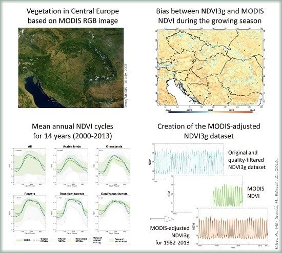
Overall (covering the entire study area) and land cover type (forests, arable lands, and grasslands) specific mean seasonal NDVI profiles calculated from NDVI3g_O, NDVI3g_F, and NDVI_MODIS are presented in Figure 1. Note that the mean seasonal NDVI profiles derived from NDVI3g_H and NDVI_MODIS are virtually the same (but the datasets differ in any other sense), as the applied harmonization creates a dataset that is equivalent with the NDVI_MODIS in terms of multiannual NDVI curves (see Section 2.5). Seasonal NDVI profiles were compared for the whole year, and also for a subset covering the growing season only (from the second half of April to the first part of September).

Considering the whole year, the overall differences in the derived multiannual NDVI curves between the NDVI3g_O and NDVI_MODIS datasets are relatively small with a median bias of −0.004 (standard deviation of the bias is 0.054), a median mean RMSE of 0.079 (standard deviation is 0.034), and a median R of 0.964 (standard deviation is 0.074). Disagreements between the profiles are clearly visible in Figure 1, which means that NDVI3g_O estimated somewhat different profiles than NDVI_MODIS. This is most pronounced during the growing season for herbaceous vegetation (croplands and grasslands). NDVI3g_O and NDVI3g_F show lower NDVI than MODIS during the dormant season (probably due to the applied snow filtering methods). Noise in the NDVI3g_O dataset is evident from the wider overall range of the individual curves.

Considering the whole year but treating land cover types separately, median RMSE between NDVI3g_O and NDVI_MODIS is 0.076 for forests and arable lands, while it is 0.085 for grasslands. Median R for forests, arable lands and grasslands are 0.961, 0.945 and 0.973, respectively. In the case of median bias, the difference is larger with values of −0.035, 0.009, and 0.024 for forests, arable lands, and grasslands, respectively.

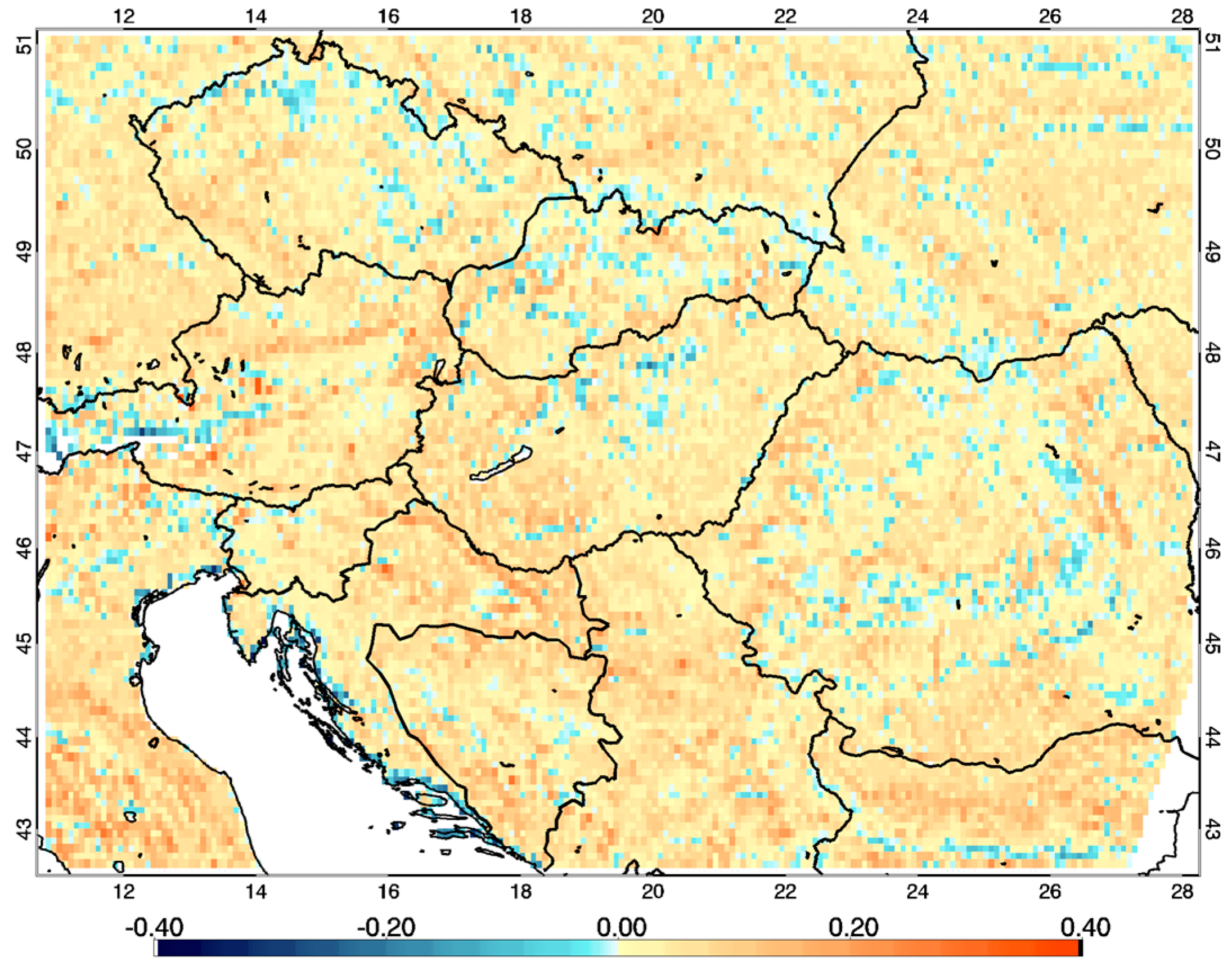
Given the large deviation between NDVI3g_O and MODIS during the dormant season, we repeated the calculations for the growing season only. Based on the multiannual NDVI curves the mean difference between the NDVI values of NDVI3g_O and NDVI_MODIS was investigated also in a spatially explicit manner for the whole study area. Figure 2 shows the map of biases for the growing season. During this time period, a positive bias (with a median bias of 0.049) was observed in 88% of the vegetated study area, while a negative difference (with a median bias of −0.017) was present at the remaining 12% of the area, where the overall median bias was 0.044, the median RMSE was 0.063 and the median R² was 0.87. Seasonal bias maps are presented in the Supplementary Material (Figure S2).

Focusing only on the growing season, median RMSE between NDVI3g_O and NDVI_MODIS is smaller (0.042 for forests, 0.069 for arable lands and 0.070 for grasslands, respectively). Median R is slightly lower for the growing season (0.893, 0.900 and 0.922 for forests, arable lands, and grasslands, respectively), while the median biases show better performance with a value of 0.001, 0.056 and 0.062 for forests, arable lands and grasslands, respectively.

During the growing season, we found a characteristic land cover dependency in some cases with high positive biases (higher NDVI3g_O compared to NDVI_MODIS) for the pixels covered by bare rocks, sparsely vegetated areas, artificial surfaces of discontinuous urban fabrics, grasslands and arable lands, while negative high biases were typical mainly for forests, arable lands, and beaches.

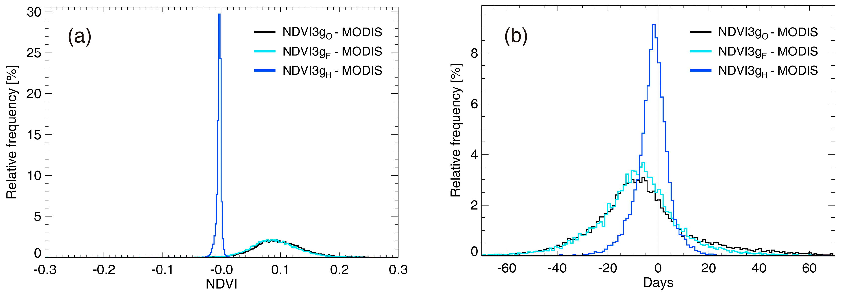
3.3. Start of the Season and End of the Season

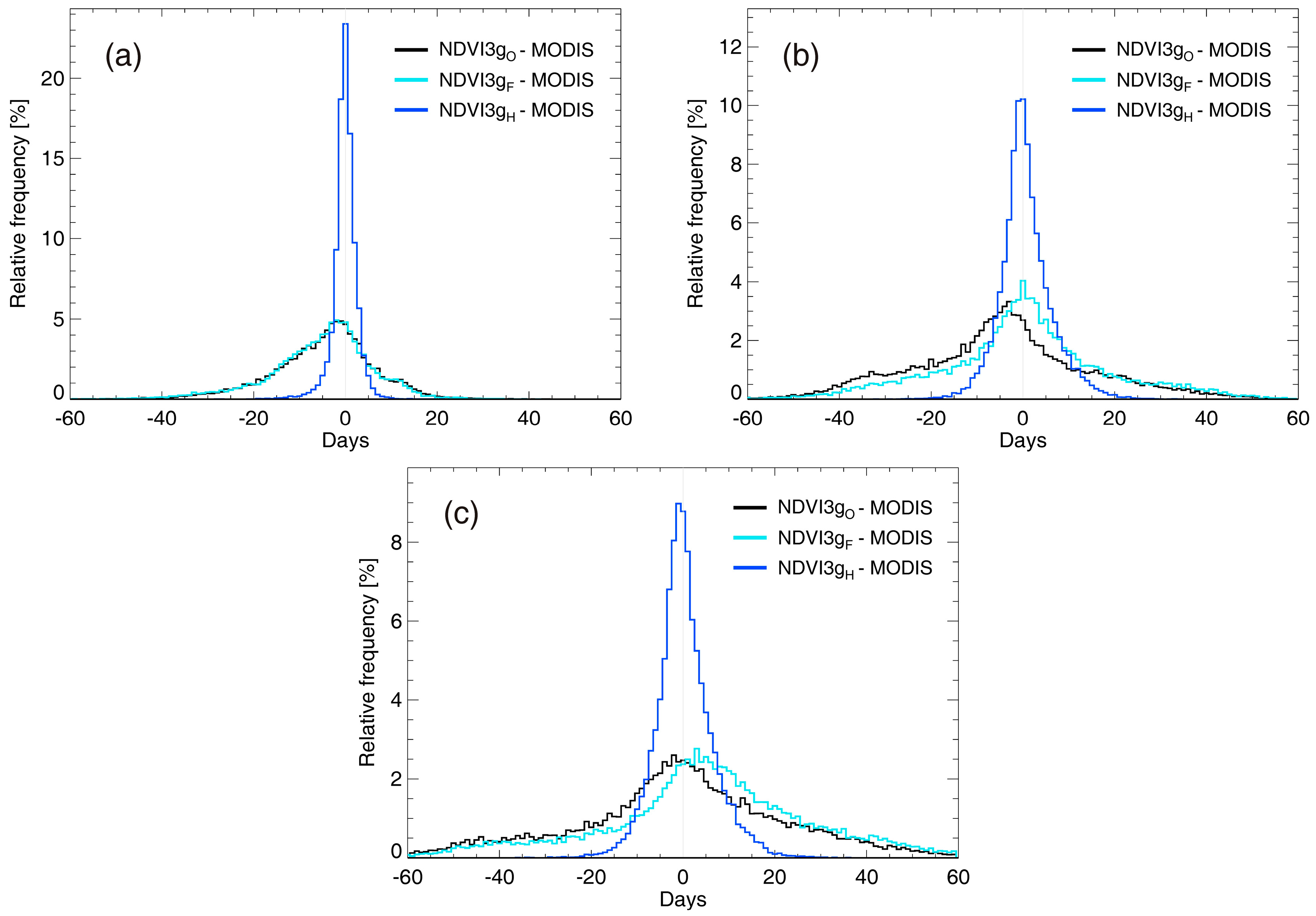
Figure 3a shows the frequency distribution of biases (Δ) in the SOS between the three NDVI3g-based datasets and NDVI_MODIS (Δ_SOS = SOS_NDVI3g − SOS_MODIS) for the study area during the overlapping years between 2000 and 2013. In Figure 3a and in the forthcoming histograms, the frequency distribution of the error metrics represents spatial variability.

We found significant variability between SOS estimated from NDVI3g_O and from NDVI_MODIS (median bias is −3 days, which means earlier growing season start for NDVI3g_O; standard deviation of bias is 11.3 days). The 5th and 95th percentiles of the bias were −24.6 and 13 days, respectively. In 18.4% of the target area, the absolute bias was less than 2 days. BISE-filtering had only slight and not necessarily positive effect on the results (median bias is −3.3 days). MODIS-based harmonization clearly improved the agreement of the NDVI3g_H dataset with respect to SOS with a median bias of 0.5 days and a standard deviation of 3.9 days. According to Figure 3a, spread of the bias decreased considerably, and in 67.8% of the area, the bias was less than 2 days. The 5th and 95th percentiles of the bias for NDVI3g_H were −3.8 and 4.2 days, respectively. Distributions of R values obtained from the correlations between the pixel-level SOS estimated with NDVI3g_(O,F,H) datasets with different level of processing and NDVI_MODIS show shifting toward higher values of R with each level of processing (see Supplementary Material Figure S5). This implies that SOS estimates from different NDVI3g datasets are getting closer to SOS from NDVI_MODIS.

The frequency distribution of EOS bias between the three NDVI3g and NDVI_MODIS datasets (Δ_EOS = EOS_NDVI3g − EOS_MODIS) is shown in Figure 3b. End of the season estimation from the NDVI3g_O is mostly biased and varies within a wide range of about 120 days (i.e., 4 months). The median bias is −4 days, while the standard deviation of bias is 19.3 days. The 5th and 95th percentiles of the bias are also rather large (−36.6 and 29.5 days, respectively). The absolute difference was less than 2 days only in 10.7% of the target area. BISE-filtering had a detectable effect on the bias (median value of 0.6 days) though the large variability decrease is only marginal. MODIS-based harmonization clearly improved the quality of the NDVI3g_H dataset respect to EOS as well (median bias of 0.6 days, and standard deviation of 5.7 days) and the resulting dataset showed a bias that scattered within ~40 days. The harmonization resulted in a dataset with bias <2 days in 37.4% of the total area studied. The 5th and 95th percentiles of the bias for NDVI3g_H were −7.5 and 11.4 days, respectively.

Considering correlations between EOS estimated from the NDVI3g_(O,F,H) datasets and EOS from NDVI_MODIS (see Supplementary Material Figure S9), the results are similar to the case of SOS. Corrections improved correlations to some extent. Supplementary Material contains additional figures on the spatial pattern of SOS, EOS bias and their R values (Figures S3, S4, S7 and S8), where the maps of R are showing only the pixels where R is statistically (p < 0.01) significant.

Land cover dependency was found in the biases of SOS and EOS (see Supplementary Material Figures S6 and S10). In case of SOS values derived from the NDVI3g_(O,F) datasets, arable lands and coniferous forests showed the highest variability of SOS and the weakest agreement with the SOS derived from MODIS data, and the harmonization modified the results to a lesser extent. For all kinds of forests generally (and especially for broadleaf forests), the agreement was considerably stronger, and the SOS values were markedly improved due to harmonization. The situation was similar in case of EOS, where arable lands showed a strong positive bias before the harmonization, which means that the NDVI3g_(O,F) datasets significantly overestimated the EOS. Land cover specific results of grasslands (and to a lesser extent of coniferous forests) should be handled with caution due to the low number of pixels.

3.4. Length of the Growing Season

In case of the length of growing season, the frequency distribution of the bias between NDVI3g_O, NDVI3g_F, NDVI3g_H and NDVI_MODIS (Δ_LOS = LOS_NDVI3g − LOS_MODIS) is shown in Figure 3c. Considerable variability is present in NDVI3g_O and NDVI3g_F, and the distribution of bias is similar to that of SOS (Figure 3a). The median bias is 0.26 days, which is in fact small, but the spread of bias is large (the 5th and 95th percentile of the bias are −43.8 and 39.4 days, respectively). After BISE-filtering the median bias increases to 5.6 days, while the standard deviation of bias hardly changes (decreases from 24.1 to 23.8 days, with similar 5th and 95th percentiles). Harmonized NDVI3g_H shows better performance (similarly to the EOS case) with close-to-zero median bias, 6.4 days standard deviation of bias, and −8.9 days 5th percentile, and 11.7 days 95th percentile values. The correlation between LOS estimated from NDVI3g_(O,F,H) and NDVI_MODIS datasets show similarities with the one of SOS and EOS (Supplementary Material Figure S13), however, the spatial pattern of biases resembles only to EOS and while it differs from SOS (Supplementary Material Figure S11).

The land cover dependency of LOS’s error (Supplementary Material Figure S14) is similar to that of the EOS’s error, which means a strong overestimation by the NDVI3g_O datasets in the case of arable lands. The highest improvement is due to harmonization in the case of forests.

3.5. Value and Timing of Peak NDVI

During the overlapping 14 year period, annual maximum NDVI was systematically higher for NDVI3g_O and NDVI3g_F than for NDVI_MODIS (Figure 4a). The median bias (Δ_peak = peak_NDVI3g – peak_MODIS) was 0.096 for NDVI3g_O and 0.089 for NDVI3g_F, while the standard deviation of bias was around 0.046 for both cases. MODIS-based harmonization substantially improved the multiannual mean maximum NDVI compared to NDVI_MODIS (Figure 4a): NDVI3g_H approached NDVI_MODIS with a median bias of −0.003 and standard deviation of bias of 0.004. The 5th and 95th percentiles of the maximum NDVI bias were −0.011 and 0.015, respectively.

Figure 4a shows that the frequency distribution of maximum NDVI bias for NDVI3g_O and NDVI3g_F are similar. This is also the case for the correlation coefficients between maximum NDVI_MODIS and the original and BISE-filtered NDVI3g_F (Supplementary Material Figure S17). The median R for NDVI3g_O (0.25) and NDVI3g_F (0.27) are small, which indicate a low ability for explaining interannual variability in maximum NDVI. MODIS harmonization improved R in such a way that the number of pixels with negative R decreased and the peak of the distribution shifted towards higher positive values.

Bias of timing in peak NDVI (Δ_timing = timing_NDVI3g – timing_MODIS) was comparable to that of EOS and LOS bias (Figure 4b cf. Figure 3b,c). Median bias was −7.4 days for both NDVI3g_O and NDVI3g_F, which means an earlier NDVI maximum estimation by the NDVI3g_O dataset by one week. The 5th and 95th percentile bias covered 71.5 days for NDVI3g_O, and it covers 55.2 days for NDVI3g_F. MODIS harmonization improved the quality of the estimation (Figure 4b), as the median bias of timing for maximum NDVI for NDVI3g_H is −1.3 days for the target area. The standard deviation of bias decreased to 7.5 days, while the time period covered by the 5th and 95th percentiles decreased to 21.6 days (cca. 3 weeks). Correlation between the timing of maximum NDVI between the reference NDVI_MODIS and the NDVI3g with different processing levels is presented in Supplementary Material Figure S21. Neither BISE-filtering nor MODIS harmonization changed the overall distribution of R within the target area.

Land cover specific results (Supplementary Material Figure S18) in case of value of the maximum NDVI reveal significant differences between arable lands and broadleaf forests, where maximum NDVI derived from NDVI3g_O dataset is considerably higher for arable lands (with a median difference of 0.094) than for broadleaf forests (with a median value of 0.039). These results are in accordance with the observed differences between the mean seasonal profiles discussed in Section 3.1. Land cover dependency for the timing of the maximum NDVI again shows considerable differences between arable lands and forests (Supplementary Material Figure S22), where maximum NDVI for arable lands occurs earlier, while for forests (especially for broadleaf forests) it occurs later based on the NDVI3g_O data.

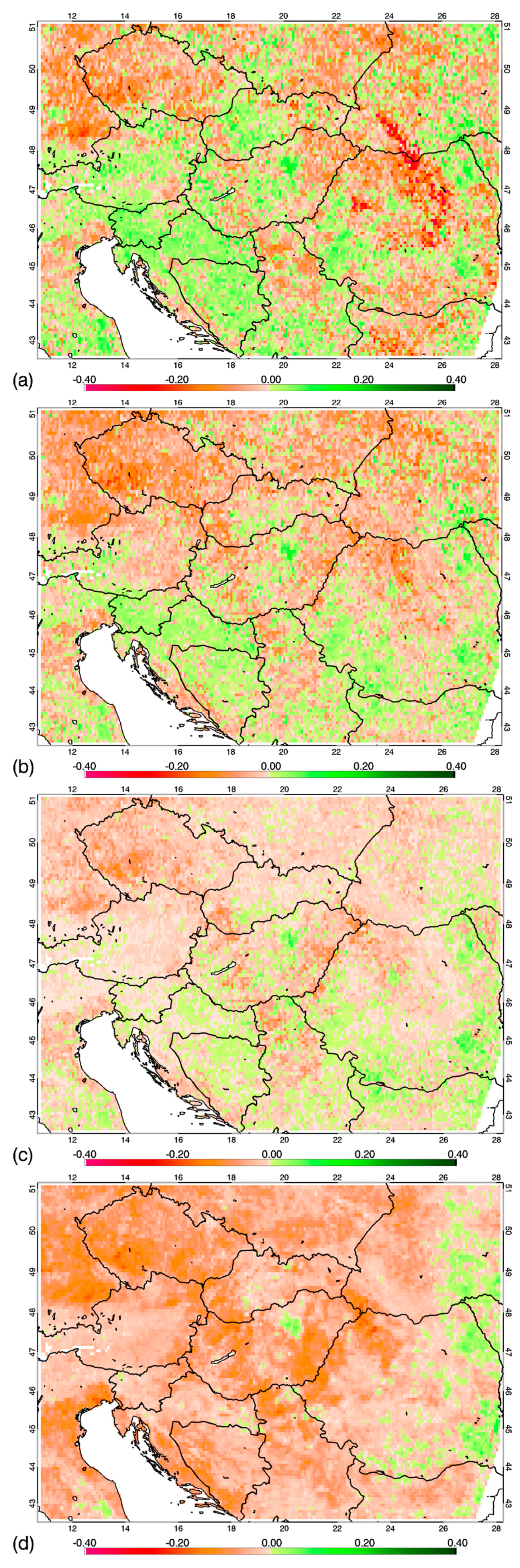
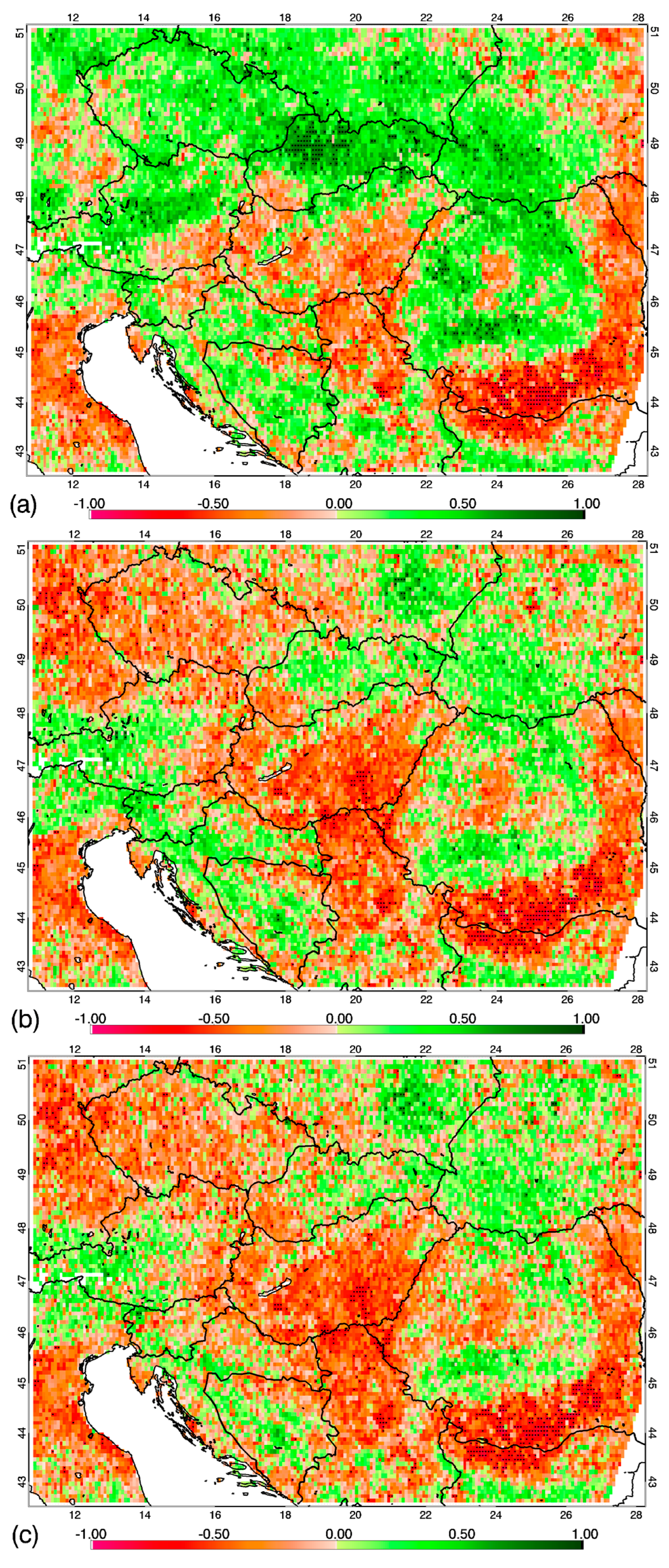
3.6. Anomaly Fields

Figure 5 shows example anomaly maps for the beginning of September 2003, after a well-documented and widely studied severe heatwave and drought spell in Europe [63,81,82]. The maps show that the original NDVI3g depicts large areas with a positive anomaly which is not realistic in comparison with NDVI_MODIS (see also maps in [82]). MODIS-based harmonization improves the overall quality of the anomaly map in terms of sign of anomaly and its spatial pattern.

NDVI_MODIS anomalies in the whole region during the overlapping 14 years were characterized by 5th and 95th percentiles of –0.071 and 0.066, respectively, while for NDV3g_O and NDV3g_H by a −0.143 and 0.128, and a −0.039 and 0.040, respectively. It means that the wide scatter of the NDV3g_O anomalies decreased for NDV3g_H.

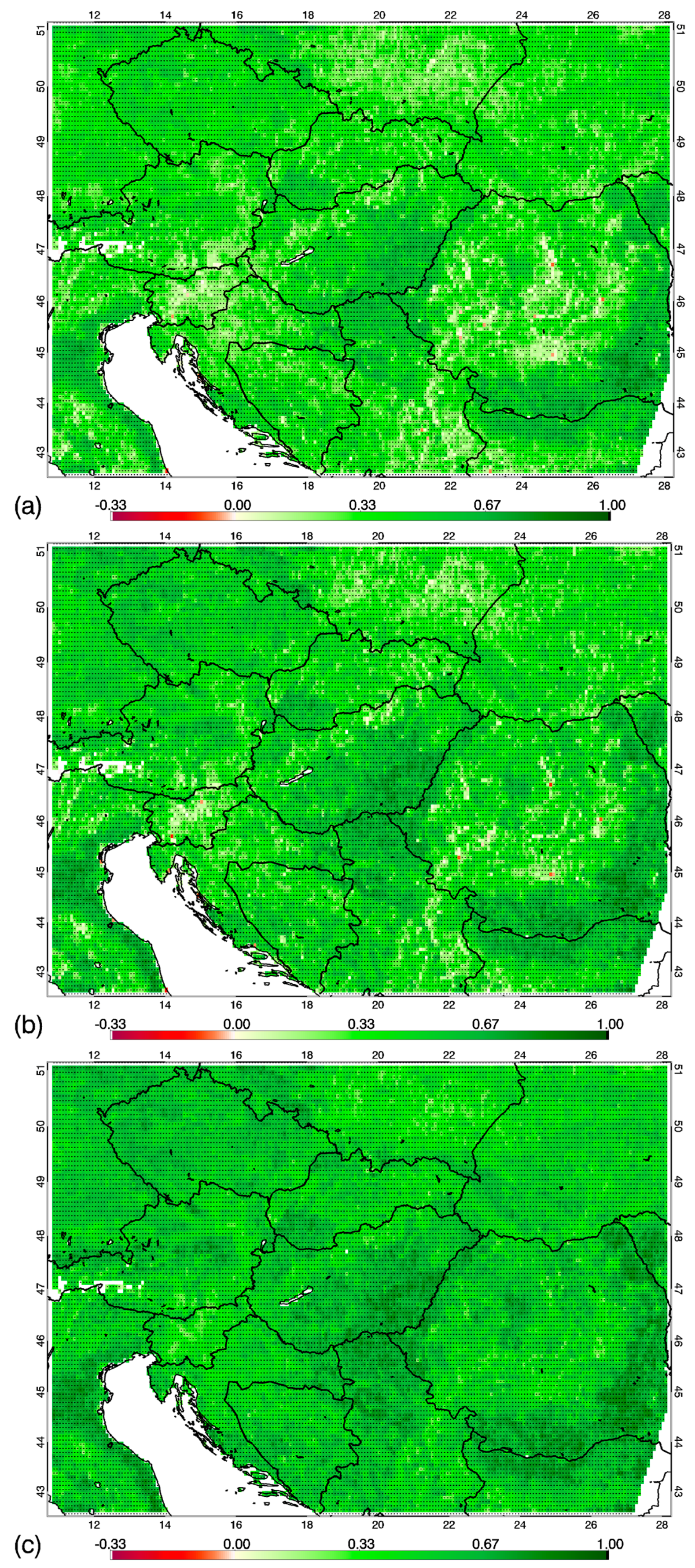
In order to check the consistency between MODIS and NDVI3g_(O,F,H) anomalies correlation coefficients were determined. The correlation coefficients between the anomalies of NDVI_MODIS and the harmonized NDVI3g_H datasets show obvious improvement compared to the original dataset during the overlapping 14 years (Supplementary Material Figure S23). Note that in case of the NDVI3g_O and NDVI3g_F the significance level is less than 0.01 if |R| > 0.14, while all R values between NDVI_MODIS and the harmonized NDVI3g_H have lower significance level than 0.01, therefore they can be handled as a statistically significant relationship.

As the non-growing season NDVI might be noisy because of the presence of snow or cloud, we investigated these correlations for the time period between the second half of April and the first part of September. The distribution of the R values is presented in Supplementary Material Figure S24. It was found that the range of the distribution was wider for the growing season, and contained more negative R values, indicating an even weaker relationship between the anomaly values for all land cover types. In case of all three NDVI3g derived datasets (NDVI3g_O, NDVI3g_F, and NDVI3g_H) |R| > 0.21 means lower significance level than 0.01. Note that there are no negative R values for the harmonized NDVI3g_H datasets.

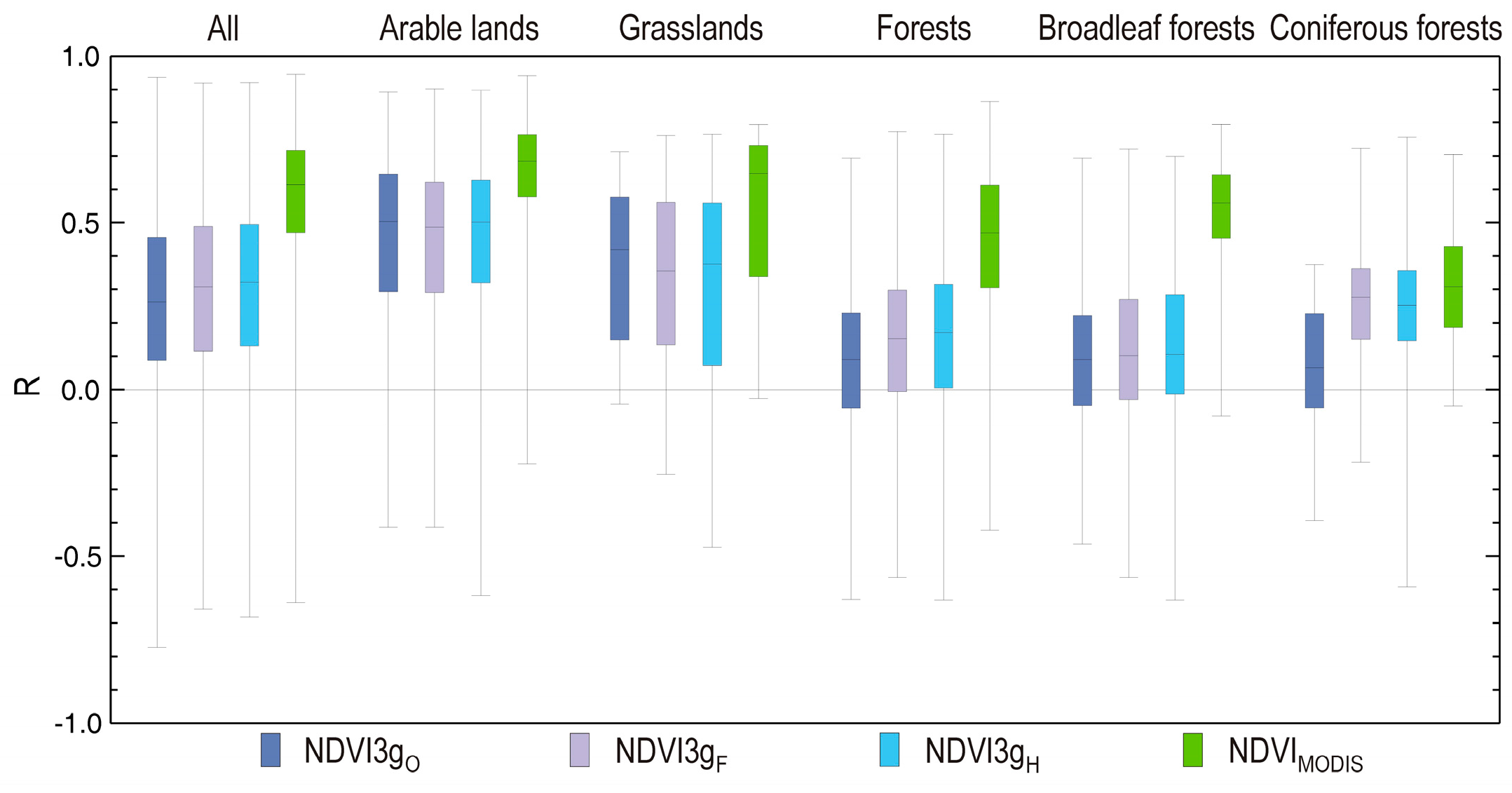
We found large differences in the R values for the different land cover types. Weaker agreement was evident for the forested pixels (relationship was the weakest for coniferous forests with a median R of 0.25 and 0.40 for NDV3g_O and NDV3g_H, respectively), and a stronger agreement for arable lands (with median R of 0.58 and 0.67 for NDV3g_O and NDV3g_H, respectively). These results are summarized in

Table 1. Statistics of the R values between the anomaly fields of NDVI_MODIS and the NDV3g_O, NDV3g_F and NDV3g_H datasets during the second half of April - the first part of September period, for all vegetated pixels and for the different land cover types. (Std. dev. of R is the standard deviation of R values).

Land Cover Type	N	Median R	5th Percentile R	95th Percentile R	Std. dev. of R
MODIS vs. NDVI3gO
All pixels	20191	0.39	0.14	0.67	0.16
Arable lands	1662	0.58	0.24	0.76	0.16
Grasslands	21	0.43	0.17	0.64	0.17
Forests	1454	0.36	0.17	0.53	0.11
Broadleaf forests	184	0.39	0.23	0.58	0.11
Coniferous forests	56	0.25	0.01	0.40	0.10
MODIS vs. NDVI3gF
All pixels	20191	0.45	0.16	0.72	0.17
Arable lands	1662	0.62	0.28	0.79	0.15
Grasslands	21	0.49	0.06	0.76	0.19
Forests	1454	0.40	0.14	0.60	0.14
Broadleaf forests	184	0.41	0.20	0.62	0.13
Coniferous forests	56	0.33	0.09	0.53	0.14
MODIS vs. NDVI3gH
All pixels	20191	0.52	0.28	0.76	0.14
Arable lands	1662	0.67	0.39	0.81	0.13
Grasslands	21	0.57	0.22	0.71	0.17
Forests	1454	0.46	0.26	0.67	0.12
Broadleaf forests	184	0.47	0.28	0.67	0.12
Coniferous forests	56	0.40	0.20	0.59	0.11

. The table shows that although BISE-filtering improves the quality of the NDVI3g dataset with shifting the original median R value (0.39) towards higher values, the harmonization shifts the total distribution in a way that it becomes narrower with an overall median R of 0.52. Maps of the R values are presented in Figure 6.

3.7. Anomalies and Their Relationship with the Climate Fluctuations

Statistical evaluation of the ability of the NDVI3g_(O,F,H) datasets to capture the magnitude and direction of the NDVI anomalies was conducted also based on the effects of climate variables, such as temperature and precipitation. The relationship between NDVI anomalies and the anomalies of the meteorological elements (expressed by the R values at pixel-level) was visualized in the form of box-whisker plots for all four datasets. This study is restricted to the growing season (from April to September) in monthly resolution.

3.7.1. Relationship between the NDVI and Temperature Anomalies

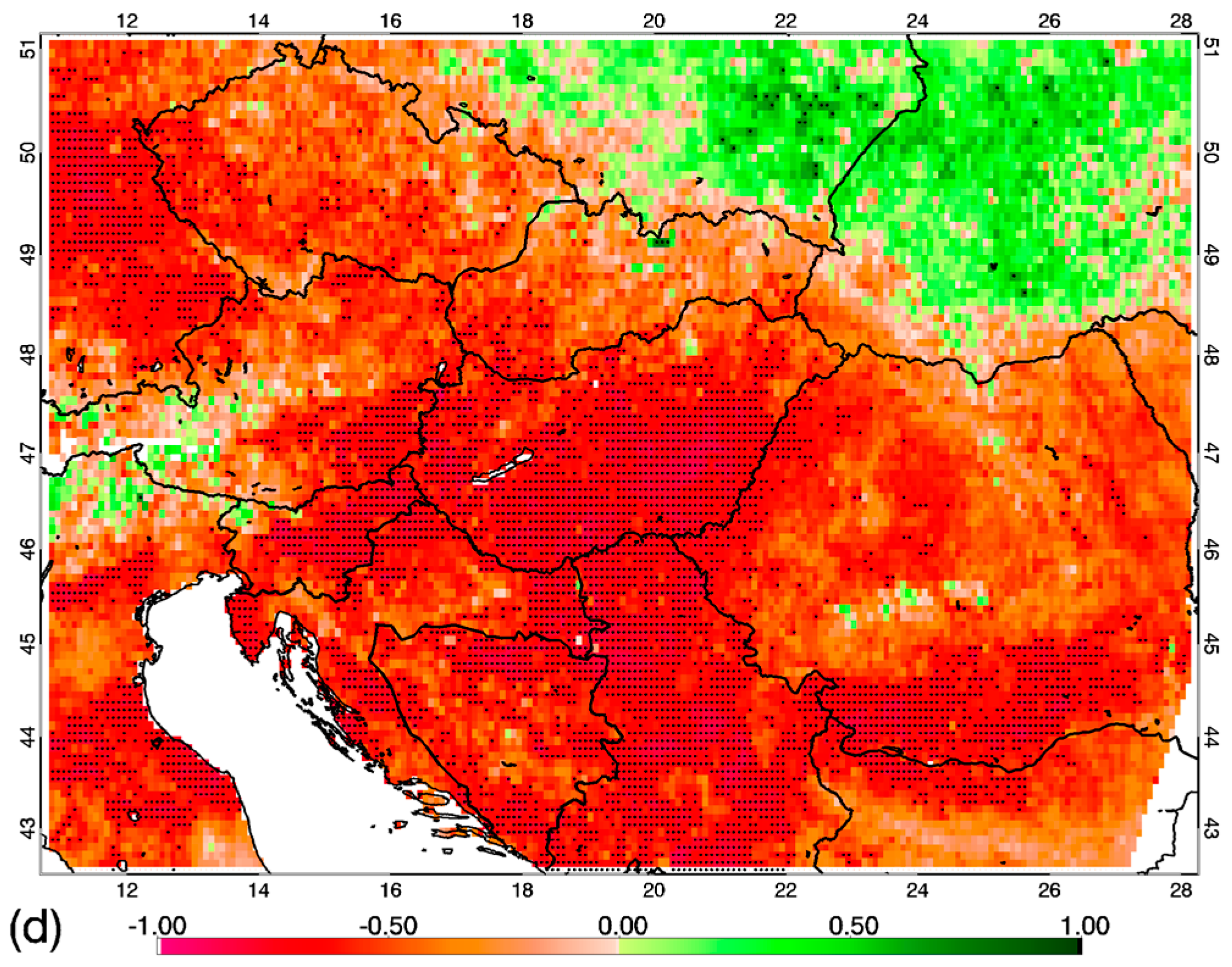
Figure 7 shows the relationship between the NDVI and temperature anomalies for August, for the entire study area, and also for the selected land cover specific pixels as well. Map of R values for the selected month are presented in Figure 8. Supplementary Material (Figure S25) contains box-whisker plots for the other months. Considering all vegetated pixels, the plot shows that the distribution of R values differ among the NDVI3g datasets with certain processing levels and from the MODIS-based data as well. Correction (BISE-filtering and harmonization) typically shifts the peak of the R distribution towards lower values (where the median R values become negative in summer), which means that the distribution gets closer to the one represented by MODIS (the latter provided the lowest, i.e., most negative R values). The scatter of R values (represented by maximum and minimum in the box-whisker plots) differ only slightly between the datasets.

Considering the specific land cover types, the gradual shift toward lower values from NDVI3g_O to NDVI3g_H is typical of all LC types. In some cases, (e.g., in May and June; see Supplementary Material Figure S25) NDVI3g_F and NDVI3g_H are very similar in terms of R distribution, which means that harmonization did not shift the R distribution toward lower values. Similarly to the case when all vegetated pixels (land cover types) were taken into account, MODIS mostly gave the lowest R values that are gradually approximated by NDVI3g_F and NDVI3g_H but are never reached. In May and June, forests exhibit different behavior, as in these two months correlation coefficients between the temperature anomaly and NDVI anomaly for MODIS show the largest R values. In May and June, BISE-filtering shifts the R distribution toward lower values, but interestingly harmonization has an opposite effect so as it shifts the distribution to higher R values (exception is coniferous forests in June), though the shift is only marginal. During this time period, distribution of R based on MODIS is more similar to the original NDVI3g_O.

3.7.2. Relationship between the NDVI and Precipitation Anomalies

Figure 9 shows the lagged relationship between the NDVI and precipitation anomalies for all LC types for September (where the effect of precipitation anomaly of August is considered), and for the specific LC types that are studied separately. Map of R values for the selected month are presented in Figure 10. Figure S26 in the Supplementary Material contains results for the other months. If the entire study area is handled as one dataset, the R values are the largest in case of MODIS. NDVI3g with different corrections are characterized by smaller R values (as shown by the 25th and 75th percentile values; note that there are exceptions), and the correction methods do not improve the result in terms of similarity with MODIS. BISE-filtering typically shifts R to lower values, where harmonization shifts them to a bit higher values. In some months (e.g., in August and September; Supplementary Material Figure S26), MODIS gives substantially different distribution.

If the different LC types are studied separately, the results show a rather heterogeneous picture. Arable lands exhibit a pattern similar to all LCs, likely due to the dominance of croplands in the study area. None of the NDVI3g based distributions provide R distribution that matches the MODIS based result. It is interesting to note the scatter among the R distributions of grasslands in June (see Supplementary Material Figure S25). In August and in September, the MODIS-based R distributions markedly differ from those represented by the NDVI3g datasets.

4. Discussion

4.1. MODIS NDVI as Reference Dataset for NDVI3g Evaluation

In our approach, the state-of-the-art Collection 6 MODIS-based NDVI dataset from satellite Terra was used as a reference to investigate the quality of the NDVI3g dataset over Central Europe. Global scale studies demonstrated the applicability of the NDVI3g, the longest available remote sensing dataset [25], in trend detection of the phenological cycle and sensitivity studies (e.g., [34,36,37,38,40,41,42,83,84,85]). Nevertheless, evaluation of NDVI3g for regional application is necessary due to known issues and uncertainties [32,33,34,35]. We chose NDVI dataset derived from the measurements of Terra/MODIS for reference because of its longer overlap with the NDVI3g dataset, relative to the one provided by Aqua/MODIS. We executed the calculations using Aqua/MODIS data (not shown here) as well, but the outcomes were similar to those from Terra/MODIS which are presented here. This corroborates the robustness and wider applicability of our results, while the selection of the MODIS NDVI dataset (between Terra and Aqua) has only marginal effect on the results, and does not influence the applied methodology.

It is important to emphasize that we do not claim that the MODIS-based NDVI is of perfect quality, as there are several other remote sensing alternatives as well for NDVI calculations (measurements of SeaWIFS, or the sensors onboard SPOT, Landsat and recently Suomi-NPP or Sentinel satellites). We only state that due to the sophisticated calibration method and quality assurance included in MODIS data processing, the derived products are of high quality. The quality of MODIS NDVI is also confirmed by results showing its consistency with ground observations [46,57,60], however, its ability to describe the phenology is dependent on land cover types [59]. Moreover, it is clear by today that MODIS NDVI became, to a certain degree, a standard with remarkable length and commonly used for inter-calibration and inter-comparison [33,34,35,36]. Researchers already use MODIS for harmonizing other datasets [63,86], and they will inevitably continue to use it as a reference.

We used maximum value compositing for the construction of our spatial and temporal resampled NDVI_MODIS dataset since this method matched best the construction of the NDVI3g data. There are other alternatives for spatial aggregation of the data (e.g., simple spatial mean or calculation from the original reflectances), but they gave similar results (not shown here). This suggests that our results are robust enough for the quality evaluation of NDVI3g. Our correction method for NDVI3g was based on quality filtering, BISE correction [71,80], and also using the so-called MODIS based harmonization. Our results should only be interpreted for these corrections. Alternative filtering and reconstruction methods are also possible (e.g., Savitzky-Golay filter, etc.; see [87]) which would inevitably provide somewhat different corrected datasets.

Collection 6 MODIS data were also used to create a novel, corrected dataset that we refer to as harmonized NDVI3g. The main reason for the creation of the harmonized dataset was to support phenology related researches in Central Europe with MODIS compatible information. Our harmonization method was implemented based on simple linear regression between NDVI3g and MODIS on pixel level for each 15-day time steps separately. This means that the seasonal variability of the difference between NDVI3g and MODIS NDVI was implicitly accounted for. In this sense, harmonization resulted in a dataset that provided the same multiannual mean NDVI seasonal profiles as MODIS/Terra did. This feature might be useful for the pre-MODIS time period (1982–1999) as we can assume that those NDVI profiles are MODIS equivalent. Mean seasonal NDVI profiles for the past might be constructed to sub-regions so that e.g., decadal changes on plant greenness can be studied based on harmonized NDVI3g_H. This feature might be useful for the detection of natural disturbance or human activity at the regional scale. MODIS comparability is emphasized here as remote sensing data users will continue to handle MODIS as the primary reference for other studies.

4.2. Phenology and NDVI Variability

Major advancement in remote sensing allows the quantification of dates of major phenological events using space-borne instruments [11,13,41,44,57,88]. It was demonstrated that in spite of their different spatial scales satellite based SOS and EOS estimations roughly match the in situ phenology observations [7,11,41,57,59,60]. Clearly, estimates based on different datasets will end up giving different dates and values for phenology events [64]. Here, we used MODIS NDVI which is one of the most popular, freely available datasets. We applied MODIS NDVI and NDVI3g with different corrections to test the applicability of NDVI3g for the detection of the beginning and cessation of the growing season, and for the estimation of the length of the vegetative period. We also studied the magnitude of annual NDVI maximum, which is an indicator of the maximum performance of the vegetation, and its timing.

The original NDVI3g-based SOS and EOS detection showed poor performance as the difference between MODIS-based and NDVI3g-based results differed by 20–30 days in the majority of the cases (EOS error was larger), without any systematic fashion. BISE-filtering [71] (see Section 2.4 and Section 2.5) did not change the overall quality of phenology timing detection. MODIS harmonization improves substantially the applicability of NDVI3g, mainly in terms of multiannual mean SOS and EOS detection. Quantification of interannual variability of spring greening and autumn senescence (i.e., year-to-year change in SOS and EOS) is somewhat problematic with NDVI3g, as even the improved dataset still shows somewhat poor performance (expressed by the correlation between the reference and the other datasets). This indicates that the harmonized NDVI3g_H is more appropriate for estimation of means but not for variability.

We used an ensemble of three methods for SOS and EOS detection, which is a common practice in the literature [62]. This means that our results can be considered as robust but inevitably depend on the choice of SOS and EOS calculation methodology. Note that the individual methods (see Section 2.9) showed similar pattern (not shown here) which corroborates that the findings are robust. Alternative methods for SOS and EOS detections are used in the literature (see e.g., [18,35,40,64]) which were not tested here due to the heterogeneity of the methods. Further studies might focus on these techniques. Our finding with earlier SOS derived from the GIMMS NDVI3g dataset corresponds to the results of Atzberger et al. [35].

Estimation of LOS with the original and BISE-filtered NDVI3g is problematic, as it provides inconsistent results in comparison to MODIS. As SOS and EOS determine LOS, errors in SOS and EOS affect the overall quality of LOS. MODIS harmonization improves the predictive ability of NDVI3g to estimate LOS. Final applicability of harmonized NDVI3g_H of the LOS is similar to that of the EOS, where both are of lower quality than the SOS. The final NDVI3g_H still has relatively large uncertainty in terms of the spread of bias. Explained variance for LOS is similar to that of SOS and EOS, and is relatively poor (R² is still typically lower than 0.5 in the whole study area).

Peak NDVI magnitude is overestimated by NDVI3g_O even with BISE-filtering, while after harmonization it gives results which are consistent with MODIS. The correlation between MODIS and NDVI3g with different corrections is still low, although MODIS harmonization causes larger improvement in terms of R with respect to SOS, EOS, and LOS.

Error in the estimation of the timing of peak NDVI is similar to the errors in the estimation of EOS and LOS. MODIS harmonization improves the ability of NDVI3g to estimate the peak NDVI timing quite well, though the time range of timing difference in the target area can span more than 3 weeks. Interestingly, R between MODIS and NDVI3g in terms of timing of maximum NDVI is unaffected by the corrections and generally shows performance which is typical for the phenology metrics already discussed.

The reliability maps presented in the Supplementary Material can support decision making on the applicability of NDVI3g for specific purposes. If the question is the estimation of the multiannual mean SOS or EOS based on NDVI3g, bias maps (Supplementary Material Figures S3, S7, S11, S15 and S19) can be useful. If the annually varying timing is to be determined with reasonable accuracy and precision, then the R-maps are good guides (Supplementary Materials Figures S4, S8, S12, S16 and S20). These reliability maps can be directly used if the entire NDVI3g dataset is evaluated in terms of phenology change or trend for specific vegetation characteristics.

4.3. NDVI Anomalies and Their Relationships with Meteorological Variables

Elucidation of the relationship between unusual plant state and climate anomalies is the subject of several ongoing research activities [14,36,62,63,89,90,91,92,93,94]. Climate effect on plant state and vigor was studied in many cases. These studies range from relatively simple regression analysis between climate variables and vegetation index anomalies [95,96] to more complex studies focusing on resilience and resistance of ecosystems [14,90]. These studies are also useful to identify sensitivity of plant communities to precipitation and temperature anomalies [93,97].

Obviously, the first step of this kind of activity is the detection of anomalies. This can be done via different remote sensing datasets and proxy variables but the quality of the retrieved anomaly fields might remain unaddressed. Therefore, a comparison of the anomaly fields is always desired, preferably with a dataset that is widely tested and verified in terms of its ability to detect anomalies.

Attribution of the detected signal is another major challenge. Understanding the response of plant production to meteorological anomalies might help project plant physiology and vulnerability under changing environmental conditions [89]. Plants growing under different climates might have different sensitivity to the same anomaly (e.g., drought or heat) due to acclimation and plasticity [90,98]. Therefore, the plant responses on large spatial scales, where a mixture of species is present, cannot be estimated easily from simple ecological considerations. Remote sensing can overcome this limitation as it provides observation based information about larger regions [90].

Well-documented anomaly cases can be used to evaluate the ability of NDVI3g to detect NDVI deviations from the long term means. The 2003 heatwave and drought caused widely recognized decline in plant production (including crop yield) and reduced carbon uptake [63,81,92]. We demonstrated that in major parts of Central Europe NDVI3g was not able to reproduce the anomaly pattern during the 2003 heat wave even after filtering, BISE correction and harmonization. Further case studies should be performed to evaluate the ability of NDVI3g to correctly detect individual anomaly fields. Statistical evaluation of the pixel based anomalies also revealed problems with the anomaly evaluation.

Our results reveal that in Central Europe positive temperature anomalies during the growing season typically negatively impact plant greenness and thus most likely foliage production (not considering of course the relationship between the temperature and SOS). If we hypothesize that MODIS captures correctly a response of plants to the heat, based on our findings, we can conclude that NDVI3g gives somewhat different results even after correction. The result implies that NDVI3g, even after harmonization, still shows weaker correlation with the temperature than MODIS. This is something one should be aware of when using NDVI3g, particularly for the period before MODIS.

The same is true in the case of precipitation anomalies where excess precipitation causes overall greening in the region and likely associated increase in the leaf production. NDVI3g users should keep in mind that their results might be distorted. Interestingly, in case of the anomaly detection and attribution BISE-filtering and harmonization do not result with a closer match to MODIS, like in the case of SOS.

4.4. Implications for Long-Term Calculations with NDVI3g in Central Europe

As it was emphasized in the Introduction, the NDVI3g dataset is a result of a combination of several NDVI datasets originating from different AVHRR sensors onboard the NOAA satellites (see Supplementary Material Table S4 for a list of NOAA satellites and their contribution to the NDVI3g dataset). Differences in satellites raise a question of how well the harmonization between NDVI3g and MODIS NDVI might be extended to the period before MODIS era. To estimate the limitations of harmonization with MODIS NDVI, a test was conducted. We performed harmonization using only part of the NDVI3g dataset originating from NOAA-17 (period 2004–2008) and compared the goodness of harmonization with MODIS NDVI for the overlapping (2004–2008) and non-overlapping (2001–2003 and 2009–2013) periods. The goodness of harmonization between NDVI3g and MODIS NDVI was quantified with RMSE, handling MODIS NDVI as a reference. Using only data of NOAA-17, the harmonization in the applied period (2004–2008) resulted in RMSE decreasing from 0.097 (NDVR3g_O) to 0.023 (NDVI3g_H), while outside of the era of NOAA-17 (non-overlapping period of 2001–2003 and 2009–2013) RMSE dropped from 0.109 (NDVR3g_O) to 0.046 (NDVI3g_H). For comparison, overall harmonization (performed by using the NDVI3g dataset for the entire MODIS era (2000–2013)) resulted in RMSE reduction from 0.122 for NDVR3g_O to 0.034 for NDVI3g_H. As expected, harmonization between NDVI3g and MODIS NDVI yields best results when it is made in a satellite-to-satellite fashion for instruments orbiting simultaneously. However, reduction in RMSE—even in the case when harmonization was performed based on different satellites and non-overlapping periods—indicates that the implementation of harmonization might be sensible also for the part of the NDVI3g dataset prior to MODIS era.

5. Conclusions

In this study, we presented an in-depth analysis of the quality and suitability of the NDVI3g dataset for the estimation of different vegetation characteristics in Central Europe. The target region covers countries with transitional economies, where the vulnerability of the ecosystems to climate change [99] is related to the ongoing management practices [100]. This means that monitoring of vegetation activity is of priority both for scientific and economic reasons.

Our results showed that the original NDVI3g has limited applicability in Central Europe. This was revealed by the significant disagreement between different vegetation state metrics (related to spatially averaged NDVI profiles, phenology and maximum greenness) derived from the original NDVI3g and MODIS NDVI datasets. This finding points to the need for further noise filtering and adjustment of the original NDVI3g dataset.

Noise reduction with the BISE method slightly improved the results but the accuracy of NDVI3g_F is still low. The harmonization of NDVI3g with MODIS NDVI is promising since the created dataset shows improved quality for phenology timing detection and the other vegetation metrics. This finding suggests that it is not the noise of NDVI3g that limits the applicability of NDVI3g for the characterization of plant state.

Anomaly detection with NDVI3g should be handled with caution in Central Europe. The ability of other datasets should be checked for alternatives. NDVI3g has some applicability in attributing NDVI anomalies to meteorological anomalies, where harmonization helps to improve the covariance between NDVI and temperature/precipitation anomalies. Still, MODIS-based results are not reproduced well, even by NDVI3g_H which warns us that results derived from NDVI3g_(O,F,H) should also be interpreted with caution.

The presented results can help researchers to assess the expected quality of the NDVI3g_(O,F,H) based studies in Central Europe. Spatially explicit reliability maps presented in the Supplementary Material can support the selection of target regions for further studies with NDVI3g where the results are in better accordance with those retrieved by MODIS. Though the present study has limited spatial extent, it was intentionally designed to focus on the size of an area that would be most interesting from a national and/or regional aspect (e.g., to policymakers, local climate change analysis/awareness raising campaigns, etc.). Nevertheless, described methods and quality metrics are generic and can be used for other geographic regions as well without modification. The applicability of our results is likely restricted to the mid-latitudes with similar climatic conditions and land cover. For other regions (e.g., the tropics or the boreal regions) similar studies can be conducted based on the presented methodology.

The quality and BISE-filtered NDVI3g and the harmonized datasets for the studied domain are available from the corresponding author. The harmonized dataset is also available at Zenodo [101].