Global Daily High-Resolution Satellite-Based Foundation Sea Surface Temperature Dataset: Development and Validation against Two Definitions of Foundation SST

Abstract

This paper describes a global, daily sea surface temperature (SST) analysis based on satellite microwave and infrared measurements. The SST analysis includes a diurnal correction method to estimate foundation SST (SST free from diurnal variability) using satellite sea surface wind and solar radiation data, frequency splitting to reproduce intra-seasonal variability and a quality control procedure repeated twice to avoid operation errors. An optimal interpolation method designed for foundation SST is applied to blend the microwave and infrared satellite measurements. Although in situ SST measurements are not used for bias correction adjustments in the analysis, the output product, with a spatial grid size of 0.1°, has an accuracy of 0.48 ${}^{\circ }$C and 0.46 ${}^{\circ }$C compared to the in situ foundation SST measurements derived by drifting buoys and Argo floats, respectively. The same quality against the two types of in situ foundation SST (drifters and Argo) suggests that the two definitions of foundation SST proposed by past studies can provide same-quality information about the sea surface state underlying the diurnal thermocline.

1. Introduction

The sea surface is the interface between the atmosphere and ocean. The temperature at this boundary, known as sea surface temperature (SST), is one of the important parameters in atmospheric and oceanographic studies and social applications. SST can be an indicator of climate change through direct and indirect effects. In addition, SST may indicate the thermal condition of the upper ocean and its influences on physical and bio-geochemical processes. Thus, detection of SST fronts can be used for applications like monitoring and reassessment of fishing grounds (e.g., [1,2]).

In recent decades, daily-step gridded SST datasets for global or regional oceans, including New Generation SST for Open Ocean (NGSST-O) for the western North Pacific area released by Tohoku University [3,4,5], have been released by several agencies and universities. Such daily-mean SST products are usually generated from multi-satellite observations in various local solar times (LSTs) within one day or within a specified time-window of a few to several days around a given day. Global SST observation by microwave radiometers with low-frequency channels (6–10 GHz) is an epoch-making invention for producing such gridded SST datasets with high spatial and temporal resolutions. This method can provide SST measurements under almost-all-weather conditions except for strong rainfall. Since the 1980s, satellite remote sensing by infrared radiometers has been used to obtain SST estimates at the skin-layer depth, which is less than 100 $\mathsf{\mu }$m; however, microwave radiometers measures the temperature at slightly deeper regions in the order of 1 mm, which is known as sub-skin SST [6]. SST measurement with an appropriate on-orbit calibration system [7] was originally launched as part of the Tropical Rainfall Mapping Mission (TRMM) Microwave Imager (TMI) with a 10-GHz band. During a one-year period, Guan and Kawamura [8] studied the influence of clouds on SST coverages by using the TMI and other infrared sensors on-board both polar-orbiting and geostationary satellites. Although infrared measurements provided 50%–60% data coverage with large seasonal variations, TMI SST coverage was 78% with no remarkable seasonal change. However, the latitudinal extent of TMI was limited between 40°N and 40°S, the 10-GHz SST measurements cannot provide accurate SST in low-temperature conditions, and influences from wind were strong at higher frequency bands (e.g., [9,10]). Therefore, global SST observation by microwave radiometers was difficult until 2002, when the Advanced Microwave Scanning Radiometer for Earth Observing System (AMSR-E) on-board Aqua and WindSat on-board Coriolis were launched for their global missions.

Diurnal variation, also referred to as intra-day variation, is a characteristic and dominant variation of SST temporal variability. Kawai and Wada [11] provided a review on diurnal SST variations and their impact on air-sea interaction. The diurnal SST variation strength is determined mainly by the amount of solar heating and the magnitude of sea surface wind (SSW). Although the average diurnal amplitude of SST is a few tenths of a degree [12], diurnal variations of several degrees in amplitude with spatially-coherent structures over large areas up to 1000 km are often observed [13,14]. The diurnal variations of upper surface temperature, however, increase during daytime usually within a top of several meters in oceans [15]. In a review of the uncertainty of in situ SST datasets, Kennedy [16] mentioned diurnal variation of temperature as one uncertainty factor and reported that variety in observation time can lead to spurious changes in the data due to the diurnal cycle of temperature. Thus, cases of such uncertainty and pseudo-variability (pseudo-SST fronts) could be contaminated in satellite-based SST data (e.g., [17]).

Donlon et al. [18] introduced the concept of foundation SST (SST${}_{\mathrm{fnd}}$), which was defined as the “water column temperature free from diurnal variation.” Their definition is referred to in the present paper as “SST${}_{\mathrm{fnd}}$ Definition (1)”. The Group for High Resolution Sea Surface Temperature (GHRSST) [6] introduced an additional definition of foundation SST: the temperature at the first time of the day when the heat gain from absorption of solar radiation exceeds the heat loss at the sea surface. This definition, which is based on the fact that diurnal thermoclines disappear at local sunrise, is referred to in the present paper as “SST${}_{\mathrm{fnd}}$ Definition (2)”. From the in situ profiling data, it was concluded [19] that these two definitions are essentially identical to each other. By employing diurnal correction on the satellite SST at various local times to the daily-minimum SST, it is expected that pseudo SST patterns will be eliminated as much as possible. Examples of existing foundation SST datasets include the Canadian Meteorological Centre (CMC) product [20] and Operational Sea Surface Temperature and Sea Ice Analysis (OSTIA) [21]. In OSTIA, the daytime SST observations with low wind speed (<6 m/s) are rejected to represent the foundation SST. Moreover, the satellite measurements are adjusted for the analyzed field to represent the diurnal-free SST in these products. For applications in oceanography, such as monitoring and reassessment of fishing grounds based on SST data, the foundation SST field would be more appropriate than the daily-mean or daily-maximum fields with contamination by the long-horizontal and thin-vertical diurnal signals, because the foundation SST can represent sub-surface structures underlying the diurnal thermocline.

This paper describes the method of blending satellite SST measurements through microwave and infrared ranges at various observation times with the gridded daily-minimum SST dataset developed by Tohoku University. A brief introduction about the method for producing the daily-minimum SST for the tropical and North Pacific regional data was presented in previous research [22]. In the present study, the daily-minimum SST, which was frequently observed at sunrise LST [14], is referred to as the foundation SST according to the definition stated previously. The diurnal correction for estimating the daily-minimum SST is employed by using other geophysical remote sensing data. Figure 1 shows an example of the foundation SST fields and the spatial gradient developed in this study. Reviews of the data (Section 2.1), integration/quality-control methods applied to the data (Section 3) and validation results of the global product (Section 4) are provided. Discussions of the advantages and limitations of this study are given in Section 5. Finally, a conclusion of this work is presented in Section 6.

2. Data

2.1. Satellite SST Data

The blended foundation SST dataset of this study used SST data observed by infrared and microwave radiometers on Sun-synchronous satellites.

Table 1. List of source SST data used in the product. LTAN: local equatorial crossing time on the ascending node; IFOV: instantaneous field of view (cross-track × along-track for microwave sensors). Note that the spatial grid size for the standard AMSR-E mapped data (Level 3) is 25 km. The 10-km gridded data from the AMSR-E were prepared for this analysis. GCOM-W1, Global Change Observation Mission-Water Satellite.

Type	Microwave				Infrared
Satellite	Aqua	GCOM-W1		Coriolis	Terra	Aqua
Sensor	AMSR-E	AMSR2		WindSat	MODIS
main band for SST	6.9 GHz	6.9 GHz	10.7 GHz	6.8 GHz	11 $\mathsf{\mu }$m
LTAN	13:30	13:30		18:00	22:30	13:30
Spatial grid size	10 km	10 km	10 km	25 km	4 km
IFOV	74 km × 43 km	63 km × 35 km	42 km × 24 km	71 km × 39 km	1 km

summarizes the sensors and their characteristics, including local observation time (local equatorial crossing time on the ascending node (LTAN)), spatial grid size and footprint size (instantaneous field of view (IFOV)). The in situ SST measurements applied for bias correction in several satellite-based SST products (e.g., [21,23,24]), were not used to produce the dataset of this study. SST measurements by Sun-synchronous satellites can provide wide data coverage, including coverage of high-latitude oceans, where observation by geostationary satellites is difficult due to large satellite zenith angles. On the contrary, the temporal interval between observations by Sun-synchronous satellites compared with geostationary measurements is limited to one or two measurements of one geographic point by one satellite per day. However, the combined use of multi-satellite measurements enabled us to produce higher data coverage with high temporal and spatial intervals of daily and less that 25 km, respectively, which are offered by two or more microwave radiometers [17]. The proposed SST dataset used two microwave radiometer series: The first is WindSat, which was developed by the Naval Research Laboratory (NRL) for the U.S. Navy and the National Polar-orbiting Operational Environmental Satellite System Integrated Program Office, and the second is the AMSR series provided by the Japan Aerospace Exploration Agency (JAXA). To capture the mesoscale disturbances less than the footprint size of the microwave radiometers in detail, infrared SST measurements by Sun-synchronous satellites were essentially necessary. We used the SST products of the Moderate Resolution Imaging Spectroradiometers (MODIS). This section provides a short review of these sensors to facilitate the discussion in subsequent sections about their use in the SST data products as blended output.

2.1.1. AMSR-E on Aqua and AMSR2 on GCOM-W1

As an international cooperation with the National Aeronautics and Space Administration (NASA), JAXA provided an AMSR-E for the Aqua Sun-synchronous satellite, which was launched on 4 May 2002. Aqua has an orbit with an altitude of 705 km and an LTAN at 13:30, which is adjacent to the LST of the daily-maximum SST. This AMSR-E was a dual-polarized microwave radiometer with six frequency channels ranging from 6–89 GHz. Because its swath width was approximately 1450 km, data coverage by the AMSR-E in one day was limited, particularly in low- and mid-latitudes. Its operation was terminated on 4 October 2011, due to an antenna rotation problem. The hot load target on the AMSR-E, which was used for on-orbit calibration of radiance received from the Earth, experienced difficulties pertaining to physical temperature non-uniformity and variation. For the AMSR-E operation, the empirical correction method was applied to estimate the effective temperature of the hot load target [25].

The AMSR2 on-board the Global Change Observation Mission-Water Satellite (GCOM-W1) was launched by JAXA on 18 May 2012, as a follow-on of the AMSR-E. The orbit of GCOM-W1 with an altitude of 700 km and LTAN at 13:30 is similar to that of the Aqua satellite. The satellites Aqua and GCOM-W1 are members of the Afternoon Constellation (A-Train) through NASA and international cooperation. The AMSR2 is a dual-polarized microwave radiometer with seven frequency channels ranging from 6.9–89 GHz. Additional, 7.3-GHz channels were equipped to help mitigate radio-frequency interference due to broadcasting from commercial satellites or ground stations. Another important improvement in AMSR2 is better thermal design of the hot load target and intensive sunlight shielding over the load, which can provide more accurate on-orbit calibration [26]. The AMSR2 standard products, defined as a product with proven accuracy in processing and distribution operations, include SST estimation based on 6.9-/7.3-GHz measurements of oceans. In addition, SST estimation from the AMSR2 10.7-GHz measurements has been provided as a research product from the Version 2.0 AMSR2 product since March 2015 [27]. Due to the low-temperature problem in the 10–11-GHz measurements, the low SST pixels estimated as less than 9 ${}^{\circ }$C are masked in the JAXA research product. The 6.9-(7.3)/10.7-GHz channels of the AMSR2 have IFOVs of 63 km × 35 km (58 km × 34 km)/42 km × 24 km, respectively. The swath width of AMSR2 is more than 1450 km [28].

Shibata [29,30,31] described the algorithm for estimating SST from these AMSR sensors. Validation studies of the JAXA SST standard products were presented in [32,33], and the initial validation results of the 10.7-GHz SST research product were documented in [34]. However, Hosoda and Sakaida (2016, in preparation) reported that the low-temperature mask and strong wind correction in the latter product are incomplete, which could cause SST estimation errors. In the quality control (QC) system integrated in this study (Section 3.2), these errors are rejected as anomalous data, and the implementation of the quality-controlled 10.7-GHz SST measurements under both clear and cloudy atmospheric conditions is shown to improve the blended output SST product.

As the pre-processing of the blended SST production, both the AMSR-E and the AMSR2 SST products were map-projected at 0.1° for the ascending/descending nodes separately.

2.1.2. WindSat on Coriolis

WindSat is a space-borne fully- and dual polarimetric passive microwave radiometer that has operated in five frequency bands from 6.8–37 GHz. WindSat was launched on the Coriolis satellite on 6 January 2003, in an 840-km Sun-synchronous orbit with an LTAN at 18:00, which means that its descending path provides measurements at 06:00 local time around the daily-minimum SST data. The 6.8-GHz channels are the most sensitive to SST and are thus used for SST estimation. The IFOV of the WindSat 6.8-GHz channels is 71 km × 39 km (http://www.remss.com/missions/windsat). WindSat’s swath width is about 1000 km. Although this narrow swath width causes slightly small data coverage compared with that of AMSR series [35], the WindSat SST product shows high quality [36]. The on-orbit calibration problem in WindSat’s hot load target, the temperature variation introduced by the Sun’s illumination, was corrected by using the physical temperatures of the gain stages in the receiver electronics [37]. Gentemann et al. [38] described an SST estimation algorithm for the WindSat measurements. We used the WindSat mapped product with a spatial grid size of 0.25° for the blended SST production.

2.1.3. MODIS Sensors on Aqua and Terra

The Terra and Aqua satellites carry a MODIS sensor, which is an imaging radiometer for both visible and infrared radiations from Earth. This instrument has 36 spectral bands ranging from 0.4–14.4 $\mathsf{\mu }$m and a wide swath of 2330 km. The IFOV of the MODIS infrared channels is 1 km. The two-band infrared measurements at the atmospheric window (wavelength of 11 $\mathsf{\mu }$m) are used for estimating both daytime and nighttime SSTs under cloud-free conditions with atmospheric corrections. A nonlinear SST algorithm for estimating skin SST is employed by the NASA standard SST product for the global ocean [39]. To produce the blended output SST data, the MODIS SST data with the best-quality flag were used. The MODIS SST product provides twice-daily (ascending/descending) SST data from each satellite with a spatial grid size of approximately 4 km.

2.2. Sea Surface Wind and Solar Radiation Data for Diurnal Correction

The diurnal warming effects in each satellite’s SST data were corrected on the bases of the empirical method developed by [17] to the daily-minimum SST by using SSW and solar radiation observation data. A brief introduction of this diurnal correction method is presented in Section 3.1.

The JAXA Satellite Monitoring for Environmental Studies (JASMES) global dataset was used for solar radiation data. This dataset provides each sensor’s daily-mean shortwave radiation maps estimated from the Sea-Viewing Wide Field-of-View Sensor (SeaWiFS) on OrbView-2 and the MODISs on Terra and Aqua. By combining the two MODISs and SeaWiFS data from JASMES, the daily mean solar radiation data with a spatial grid size of 0.05${}^{\circ }$ were prepared for diurnal correction.

As for the SSW data in the diurnal correction for microwave SST (i.e., AMSR-E, AMSR2 and WindSat SST observations), the simultaneous SSW data from each microwave radiometer were used for calculation. For the MODIS infrared SST data, the daily-mean SSW maps were calculated for each date by using multiple satellite SSW observations. The data for the daily-mean SSW maps were collected from microwave radiometers, including AMSR-E, AMSR2, WindSat and the Special Sensor Microwave Imager (SSM/I) and Special Sensor Microwave Imager Sounder (SSMIS) series on the Defense Meteorological Satellite Program (DMSP) satellites. The last series includes the SSM/I sensors on DMSP F13, F14 and F15, and the SSMIS sensors on DMSP F16 and F17. The diurnal variation in the SSW at the fixed point would be a cause of estimation errors or artificial patterns in the produced SST product, such as a straight line at the edges of the radiometer swaths. In this study, we expected that such erroneous patterns would be removed by the QC method in the data integration schemes. The QC method used prior to the optimal interpolation (OI) operation is described in Section 3.2.

2.3. Sea Ice Data

Sea ice masks/flags are provided in the product, the methods of which are described in Section 3.4. For the Northern Hemisphere, reference sea ice data produced from measurements by visible and microwave sensors and in situ observations are used. Ice/snow flag data from the Interactive Multisensor Snow and Ice Mapping System (IMS) Daily Northern Hemisphere Snow and Ice Analysis [40] were used. The IMS dataset is derived from satellite and in situ data by the National Ice Center (NIC)/National Snow and Ice Data Center (NSIDC). The list of input data is given on the NSIDC website (http://nsidc.org/data/docs/noaa/g02156_ims_snow_ice_analysis/). The 4-km spatial grid IMS data (Version 1.2) are available for the period beginning on 23 February 2004. For analysis prior to that period, we used the Version 1.1 IMS product, which has provided 24 km ice/snow flag data since February 1997. The temporal intervals of both versions are daily.

Ice masking/flagging in the Antarctic Ocean is conducted by using microwave radiometers ice concentration data. The sea ice concentration data derived from AMSR-E and AMSR-2 [41] with a spatial grid size of 12.5 km are used primarily for the masking and flagging. In the gap period between AMSR-E and AMSR2 observations from 3 October 2011–2 July 2012 and for the dates for which AMSR-E observations were not available (

Table 2. List of dates on which the AMSR-E/AMSR2 sea ice data were not available and alternative sensors used for sea ice detection. SSM/I, Special Sensor Microwave Imager; SSMIS, Special Sensor Microwave Imager Sounder.

Period	Alternative Data
30 October–6 November 2003	SSM/I F13
19 November–20 November 2004	SSM/I F13
17 November and 21 November 2005	SSM/I F13
17 November–19 November 2006	SSM/I F13
28 November and 2 December 2007	SSM/I F13
2 February and 3 February 2010	SSM/I F13
3 October 2011–2 July 2012	SSMIS F17

), the sea ice concentration data by SSMI/DMSP-F13 and SSMIS/DMSP-F17 [42] were used. Because the spatial grid size of the SSM/I and SSMIS data at 25 km is larger than that of the AMSR-series product, the sea ice area (mask/flag) including these dates is expected to show abrupt changes due to the spatial resolution of the source data.

2.4. In Situ Data for Validation

In this study, in situ observations of foundation SST were used for the validation of both the satellite SST products and the blended output SST product. As described in Section 1, two types of foundation SST definitions are given. We used these two types of SST measurements as follows.

In situ observations of SST obtained from the Version 2.0 NOAA in situ Quality Monitor (iQuam; [43,44]) were used for validating the SST products. >From this in situ dataset, we derived the foundation SST data determined by the “SST${}_{\mathrm{fnd}}$ Definition (2)” described in Section 1. The QC for in situ SSTs, including basic screening, duplicate removal, plausibility, platform track, and SST spike checks, was performed by the NOAA iQuam system. The best quality flag data by the iQuam were used in this study. We used the Global Telecommunication System (GTS) drifter buoy data as from the iQuam database sea-truth data. The buoys with temporal sampling less than or equal to 1 h were selected for validation. In this study, from the time series by a given buoy, the daily-minimum SST was determined as the foundation SST in this study as follows: If diurnal warming was observed by a given buoy, the minimum SST at about local sunrise (06:00 LST ± 2 h) was selected as the foundation SST measurement by the buoy for the date. If the SST decreased monotonically or significant diurnal warming was not detected, the minimum SST during daytime was selected as the foundation SST observation. This last condition was introduced for consistency with the data integration operation of the satellite remote sensing, as is described in Section 3. If the position change of the drifting buoy during daytime was larger than 0.2°, the comparison was no performed in order to avoid any temperature changes caused by crossing an SST frontal structure.

In addition to the surface observation by drifting buoys, subsurface temperature profiling data recorded by Argo floats were used for validation. This in situ dataset corresponds to the foundation SST measurements of the “SST${}_{\mathrm{fnd}}$ Definition (1)” described in Section 1. Although Argo near-surface temperature data have been used recently for satellite SST validation in some studies (e.g., [45,46,47]), the Argo temperature measurements were generally difficult to apply to such uses, because typical Argo float data sampling is normally stopped at a depth of about 5 m below the surface to avoid damage. However, Castro et al. [48] used a specific subset of the Argo profiling data that includes near-surface, high vertical resolution temperature measurements in addition to that at standard depths. They manually determined the foundation SST from near-surface-temperature profiles as the temperature at the shallowest depth below the surface warmed layer. On the basis of their study, an automated method was developed in the present study for detecting the foundation SST from near-surface-temperature profiles. The advanced automatic QC Argo data (AQC) of the Japan Agency for Marine-Earth Science and Technology (JAMSTEC) provided the near-real-time Argo profile data with quality information (ftp://ftp2.jamstec.go.jp/pub/argo/AQC/). First, the temperature profiling data with good-quality flags in the ascending direction were selected. To capture the near-surface stratification (or diurnal thermocline), temperature profiles with more than seven observations in the upper 10-m depth and the shallowest observation available at a depth no deeper than 1 m were used for analysis. Vertical temperature interpolation by the Akima spline method [49] was conducted to provide 1-m interval profile data for a depth of 1–20 m, and the vertical temperature gradients $\partial T/\partial z$ were calculated. If the vertical temperature gradients were less than 0.1 ${}^{\circ }$C/m over a depth of 3 m, the temperature at the shallowest depth of this isothermal layer was determined as the foundation SST. Figure 2a presents an example of foundation SST determination from Argo profiling data. The satellite-based foundation SST and the difference between the daily maximum and foundation SST derived (Figure 2b,c) show good correspondence with the foundation SST and the derived Argo data. The Argo profiling data used for validation were gathered over the global ocean from 2012–2015.

The collocated satellite/in situ (both drifters and Argo) match-ups were generated. The nearest-neighboring satellite SST to a given in situ measurement was selected for comparison. For infrared SSTs, the spatial distance between satellite and in situ measurement should be less than 5 km. For microwave SSTs (AMSR-E, AMSR2 and WindSat), the in situ observations in coastal oceans (distance from coasts < 60 km) were removed prior to the comparison. Additionally, the spatial distance between collocated data should be less than 10 km for the AMSR series and 25 km for the WindSat observations. The difference in collocation condition is attributed to the spatial grid size of the satellite remote sensing products. The comparisons for each sensor against in situ observations were conducted by deriving the collocated data from diurnally-corrected (foundation SST estimation) or the non-corrected (daily-mean) daily-composite of each sensor. The comparison between the satellite-based blended output foundation SST and in situ measurements was conducted if the spatial distances were less than 10 km.

3. Data Integration and Quality Control

The data integration system in this study consists of diurnal correction of satellite measurements (Section 3.1), frequency-splitting and QC (Section 3.2), and OI (Section 3.3). The flowcharts of the processing system are summarized in Figure 3 and Figure 4.

3.1. Diurnal Correction

An empirical method for correcting the diurnal warming and nocturnal cooling effects in daytime and nighttime SST observations was described in [17]. The daily minimum SST was most frequently measured by the drifting and moored buoys at about 06:00 LST including mid- and high-latitude oceans [14]. The daily-minimum SST data are called as the foundation SST estimates in this study as a candidate. The diurnal correction equation used to derive the daily-minimum SST is based on the diurnal SST variation research [50], as follows:

$$\begin{array}{cc}{\mathrm{SST}}_{\min }=\hfill & c_0+c_1{\mathrm{SST}}_{\mathrm{sat}}+c_{2}ln\left(\mathrm{SSW}\right)\hfill \\ & +c_3{\mathrm{SR}}^2+c_4{\mathrm{SR}}^{2}ln\left(\mathrm{SSW}\right),\hfill \end{array}$$

(1)

where ${\mathrm{SST}}_{\min }$ is the daily-minimum SST, SR is the solar radiation, SSW is the sea surface wind speed, and ${\mathrm{SST}}_{\mathrm{sat}}$ is the satellite remote sensing observation of SST at its observation time. The temporal window for satellite SST observations (${\mathrm{SST}}_{\mathrm{sat}}$) corrected to daily-minimum SST (${\mathrm{SST}}_{\min }$) by this scheme (Equation (1)) is ±half-day around the local solar time sunrise. This diurnal correction method, which is parametrized by solar radiation and wind speed only, cannot significantly represent cooling after sunrise. Under such conditions, the cooled temperature at sea surface measured by satellite remote sensing during the local afternoon could be the minimum SST. It is debatable whether the correction method from the lower SST during daytime to SST at local sunrise is required. Further consideration is needed regarding the application of the daily gridded SST datasets. The coefficients $c_0$–$c_4$ were derived from the match-up data between in situ daily minimum SST and satellite measurements; these coefficients were individually determined for estimating daily-minimum SST (${\mathrm{SST}}_{\min }$) at drifting buoy observation depths from each satellite measurements (${\mathrm{SST}}_{\mathrm{sat}}$). The validation of the results for diurnally-corrected SST measurements at each sensor will be described in Section 4.

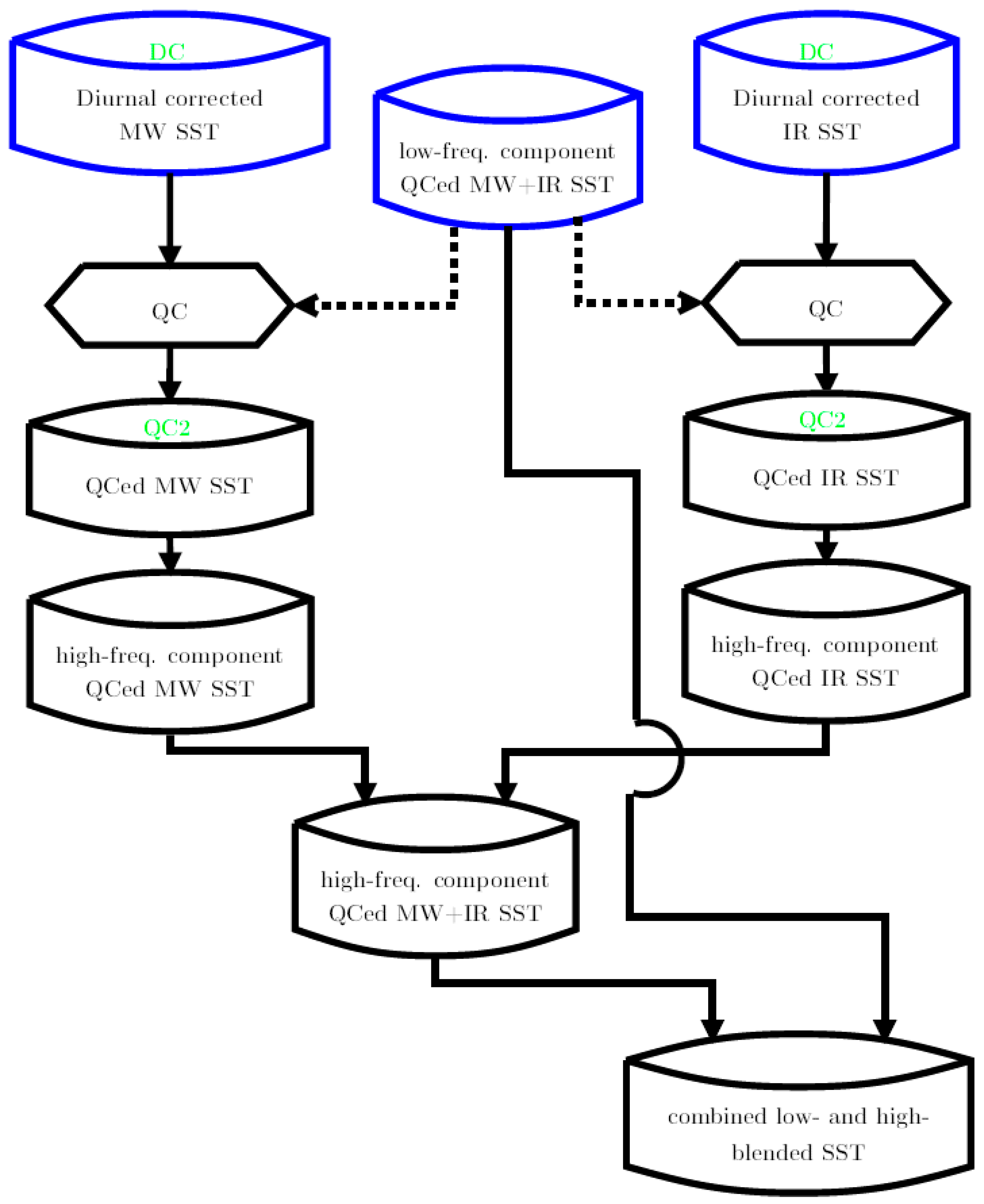
3.2. Frequency Splitting and Quality Control of SST

A temporal spectral analysis of the SST variation in the global ocean [14] revealed that the SST temporal variation could be divided into low- and high-frequency components. The former includes the interannual to semi-annual frequency range, whereas the latter consists of intraseasonal variation. To extract a first-guess low-frequency component at each grid point, a two-frequency (annual and semi-annual) windowed sinusoidal harmonics curve fitting was applied to the time series of the microwave 6-GHz diurnally-corrected SST (i.e., daily SST${}_{\mathrm{fnd}}$ data from the AMSR-E, AMSR2, and WindSat radiometers). The method performed by a least-squares fitting was described by [14], in which a half power point of the employed low-pass filter was found for a 130-day period. The amplitude and phase for the least squares fitting of the annual/semi-annual periods were estimated from time series with ±185-day/±92-day periods around the given date. This method is similar to that of the Morlet wavelet filter with a setting of high-temporal and low-frequency resolution, which enables this low-pass filter to include the interannual signal as the modulation of amplitudes and phases.

Figure 5 shows an example of the frequency splitting in this study. The original, non-filtered foundation SST field on 21 May 2005, derived by daily composite of microwave (AMSR-E and WindSat) and infrared (MODIS) foundation SST estimations, is given by Figure 5a. By employing the low-pass filter for temporal direction, the large-scale (e.g., gyre and major current such as the Kuroshio) and quasi-steady mesoscale structures (including the existence and main structures of current meanders and mesoscale eddies) were extracted as the low-frequency component (Figure 5b). The high-frequency components included transient phenomena, such as intrusions of warm and cold waters at north of the Kuroshio Extension (northeastern area of Figure 5d), deformations of the meander (southwest area of Figure 5c, where the warm waters were found around the meander) and the surrounding warm waters near a cold mesoscale eddy (eastern central area of Figure 5d). As described in the following section, the temporal scales of the high-frequency component were in the range of 3–4 days.

The quality-check process for both infrared and microwave SST data was conducted on the basis of the first-guess microwave low-pass filtered SST data. Anomalous data of SST were rejected if the following condition was not satisfied:

$$\begin{array}{ccc}\hfill \left|\right|{\mathrm{SST}}_{\mathrm{MW}/\mathrm{IR}}-{\mathrm{SST}}_{\mathrm{low},\mathrm{MW}}\left|\right|& \le & 3{\sigma }_{\mathrm{intra}.}(\mathbf{x},\mathrm{M}),\hfill \end{array}$$

(2)

where ${\sigma }_{\mathrm{intra}.}(\mathbf{x},\mathrm{M})$ is the standard deviation of the intra-seasonal SST variation with temporal and spatial intervals of monthly and 0.25°, respectively. The standard deviation of the intra-seasonal SST variation was calculated in [14]; examples of the seasonal statistics are shown in Figure 5 in that paper. The typical value of ${\sigma }_{\mathrm{intra}.}(\mathbf{x},\mathrm{M})$ is 0.6 ${}^{\circ }$C on the global average, and is in the range of 0.25 ${}^{\circ }$C–1.3 ${}^{\circ }$C. After this quality check, the low-pass filter was applied again to the diurnally-corrected infrared and microwave SST time series to produce quality-controlled, low-frequency, blended components ${\mathrm{SST}}_{\mathrm{low},\mathrm{MW}+\mathrm{IR}}$ (Figure 3).

The high-frequency component was calculated by subtracting ${\mathrm{SST}}_{\mathrm{low},\mathrm{MW}+\mathrm{IR}}$ from the original (i.e., not filtered) diurnal-corrected SST. A quality control method similar to Equation (2) is applied before the calculation of the high-frequency component, by replacing the first-guess microwave low-pass filtered data ${\mathrm{SST}}_{\mathrm{low},\mathrm{MW}}$ with the blended quality-controlled low-frequency component ${\mathrm{SST}}_{\mathrm{low},\mathrm{MW}+\mathrm{IR}}$ (Figure 4).

3.3. Optimal Interpolation

The decorrelation scales for the daily-minimum SST were calculated by [14] for each month with a spatial interval of 0.25°. The average spatial and temporal scales were determined to be about 150–400 km and 3–4 days. The analysis showed that the spatial/temporal scales in areas with high eddy kinetic energy (EKE), which was derived from the sea surface height by satellite altimeters, are relatively short/long compared to those in areas of low EKE, respectively. This suggests that oceanic perturbations with the mesoscale would be reproduced with efficiency by using such decorrelation scales. In this data integration process, the data search window for OI is ±1° in the spatial directions and ±3 days in the temporal direction.

A sub-sampling method was applied to the microwave SST data. By using simultaneous observations by microwave and infrared radiometers on the Advanced Earth Observing Satellite II (ADEOS-II), it was pointed out [51] that a large footprint size of microwave radiometer provides blurred SST images. This could be a critical problem for reproducing SST, particularly in oceanic eddy-rich areas (e.g., the western boundary currents including the Kuroshio and Gulf Stream). The brightness temperature observed by one channel of a microwave radiometer represents a complex weighted average temperature on Earth’s surface within its IFOV range. Therefore, the effective spatial resolution in the microwave SST data is determined by the IFOV sizes of the main channel for SST estimation. In addition, the almost-all-weather observations of SST by microwave radiometers could provide “excessively denser” SST data because of their high sampling rate of about 10 km, compared with infrared high-resolution SST measurements available under only clear-sky condition.

The sub-sampling method applied for microwave SST data, to reduce their excessively denser data influences on the blended output product, is similar to that adopted in the daily-mean NGSST-O Version 1.6 product [5], in which the sub-sampling rate was determined by the spatial grid size of the provided mapped products (i.e., 0.25° for both AMSR-E and WindSat). In this foundation SST product, the sub-sampling size for each microwave SST product is dependent on the IFOV size of the main channel for SST estimation. That is, the sub-sampling rates for AMSR2 6.9 and 10.7 GHz are different. If the infrared data coverage in the data search window were too scarce to solve the inverse matrix in the OI process, the sampling rate of the microwave data was changed stepwise to half or a quarter depending on the infrared data coverage (33%/16%). The OI matrix calculation in the NGSST series has been described by Guan and Kawamura [3].

3.4. Flag Information

Flag and masking information at each grid point in the blended output foundation SST product is provided for users to determine the data reliability at the given grid. For the Northern Hemisphere, a grid point is flagged as sea ice if at least one IMS grid point within a radius of 10 km is flagged as sea ice. For the Southern Hemisphere, the sea ice flag is denoted if the sea ice concentration in the microwave observations (AMSR-E, AMSR2 or SSM/I data described in Section 2.3) in the nearest-neighbor point is not zero. Sea ice flag information about the operation date and the adjacent date (±1 day) is contained in each daily supplementary flag information file. To avoid a pseudo-ice flag under severe atmospheric conditions, known as the “weather effect” in sea-ice remote sensing (e.g., [52]), a grid point in the SST product is masked as sea ice only if sea ice was detected during three consecutive days. This action is based on the assumptions that the movement of sea-ice is not very fast and that the weather effects caused by atmospheric disturbances are not temporally. persistent. Sea ice flag information uses three binary digits in each daily supplementary flag information file. If users wish to eliminate all suspicious “sea-ice” grid points in the output product, the flag information in the supplementary file could be helpful.

As is discussed (Section 4), the quality at a specific grid point in the produced dataset depends on the infrared data coverage for the grid point. In our blended SST product, the data coverage information by infrared sensors is provided as a flag in two binary digits, such as: 00: more than 50%; 01: 25%–50%; 10: 10%–25 %; and 11: less than 10%.

4. Validation

Table 3. Statistics of the validation results of satellite SSTs (non-diurnally corrected, diurnally-corrected with/without QC) against in situ foundation SST measurements by drifting buoys.

	AMSR-2		AMSR-E	WindSat	MODIS
	6 GHz	10 GHz	6 GHz	6 GHz
non-diurnally corrected (original daily-composite)
Bias	0.17 ${}^{\circ }$C	0.32 ${}^{\circ }$C	0.17 ${}^{\circ }$C	0.10 ${}^{\circ }$C	−0.05 ${}^{\circ }$C
RMSE	0.67 ${}^{\circ }$C	1.03 ${}^{\circ }$C	0.65 ${}^{\circ }$C	0.60 ${}^{\circ }$C	0.68 ${}^{\circ }$C
diurnally corrected without QC
Bias	0.03 ${}^{\circ }$C	0.23 ${}^{\circ }$C	0.01 ${}^{\circ }$C	0.02 ${}^{\circ }$C	−0.03 ${}^{\circ }$C
RMSE	0.53 ${}^{\circ }$C	1.01 ${}^{\circ }$C	0.56 ${}^{\circ }$C	0.58 ${}^{\circ }$C	0.57 ${}^{\circ }$C
Number	872,607	727,688	2,312,967	2,469,220	1,467,646
diurnally corrected with QC
Bias	0.03 ${}^{\circ }$C	0.05 ${}^{\circ }$C	0.00 ${}^{\circ }$C	0.02 ${}^{\circ }$C	0.02 ${}^{\circ }$C
RMSE	0.44 ${}^{\circ }$C	0.45 ${}^{\circ }$C	0.48 ${}^{\circ }$C	0.43 ${}^{\circ }$C	0.47 ${}^{\circ }$C
Number	686,845	526,752	1,781,611	1,295,446	693,438

and

Table 4. Same as Table 3, but against in situ foundation SST measurements by Argo floats.

	AMSR-2		AMSR-E	WindSat	MODIS
	6 GHz	10 GHz	6 GHz	6 GHz
non-diurnally corrected (original daily-composite)
Bias	0.13 ${}^{\circ }$C	0.24 ${}^{\circ }$C	N/A	0.02 ${}^{\circ }$C	−0.06 ${}^{\circ }$C
RMSE	0.61 ${}^{\circ }$C	0.96 ${}^{\circ }$C	N/A	0.60 ${}^{\circ }$C	0.64 ${}^{\circ }$C
diurnally corrected without QC
Bias	0.05 ${}^{\circ }$C	0.11 ${}^{\circ }$C	N/A	0.01 ${}^{\circ }$C	−0.04 ${}^{\circ }$C
RMSE	0.57 ${}^{\circ }$C	0.82 ${}^{\circ }$C	N/A	0.55 ${}^{\circ }$C	0.58 ${}^{\circ }$C
Number	39,338	38,354	N/A	37,712	31,860
diurnally corrected with QC
Bias	−0.04 ${}^{\circ }$C	−0.02 ${}^{\circ }$C	N/A	−0.07 ${}^{\circ }$C	0.11 ${}^{\circ }$C
RMSE	0.49 ${}^{\circ }$C	0.48 ${}^{\circ }$C	N/A	0.49 ${}^{\circ }$C	0.54 ${}^{\circ }$C
Number	31,765	28,979	N/A	19,788	28,789

show the validation results of SSTs from each sensor against the in situ foundation SST observations by drifting buoys at 06:00 LST and Argo profiling data, respectively. The statistics were calculated from the daily-composite SST from each sensor. Without diurnal correction, the microwave SST measurements (AMSR-E, AMSR2 and WindSat) showed positive biases. The large positive bias in the AMSR2 10.7-GHz measurements is attributed to the low-temperature mask errors in the original product. These noises are reduced by the QC process used in the production of the dataset. The global statistics using the two independent types of in situ foundation SST measurements in this study confirmed that the satellite-based estimates with diurnal correction can provide foundation SST fields with no significant difference between them.

The validation statistics of the blended foundation SST dataset against drifting buoys and Argo floats are summarized in Figure 6, in which histograms of the match-ups of satellite-based minus in situ foundation SST are shown together. The biases of the foundation SST in this product were less than 0.05 ${}^{\circ }$C, and the root-mean-square of errors (RMSEs) against buoys and Argo floats were 0.48 ${}^{\circ }$C and 0.46 ${}^{\circ }$C, respectively. Although bias correction using in situ measurements was not adopted in this study, the diurnal correction and iterative QC provided high-quality SST fields. Prior to the comparison against the drifting buoy measurements, the fast-moving in situ data were eliminated since the diurnal SST change by the weather conditions was not able to be distinguished from that by crossing ocean frontal structures. This occurred since the daily-minimum SST observation by a drifting buoy has ambiguity on the position for one day. The numbers of drifting buoy match-ups (Figure 6b) were reduced in the tropical oceans due to this constraint. On the contrary, the match-up distribution from Argo profiling data (Figure 6c) was not affected by the surface current constraint. However, it should be noted that adequate and uniform distributed data of near-surface Argo profiling measurements around global oceans have not been available thus far.

Figure 7 shows the geographical distributions of the standard deviation of estimating errors by the satellite blended foundation SST product, compared with in situ drifting buoy foundation SST. The calculation was conducted in each 5° × 10° (lat. × lon.) box, for the low-frequency data (Figure 7a) and the final combined low- and high-frequency components (Figure 7b). The small standard deviation of estimating errors indicates that the satellite-based foundation SST product reproduced the in situ SST fields with high accuracy. In the low-frequency component, the standard deviations in the boundary current areas (e.g., the Gulf Stream and Agluhas) and the oceans near the Antarctic (about 60°S) were as much as 1.5 ${}^{\circ }$C. The tropical oceans in the eastern Pacific, where SST spatial gradients are strong with dominant short-term variability (tropical instability waves) [53], also showed large standard deviations of about 1.2 ${}^{\circ }$C. After combining the low- and high-frequency components, the standard deviations in these areas were reduced to no more than 1 ${}^{\circ }$C. This suggests that the high-frequency perturbations in the foundation SST are active in these areas and that they are reproducible by OI by using appropriate decorrelation scales.

Figure 8 shows time series of validation statistics (bias and RMSE) calculated from the global ocean. The statistics against buoys and Argo floats were obtained on monthly and semi-annual bases, respectively, because the Argo near-surface observation data were not adequate. No abrupt change of bias was noted in October 2011, when the AMSR-E stopped its operation at LST afternoon. This indicates that diurnal correction can reduce inappropriate influences of the various local solar observation times on the daily-step, high-resolution SST datasets. However, the RMSEs from October 2011–June 2012 were slightly larger, because the available microwave SST measurements during this period were provided only by WindSat. This suggests that it is difficult to capture the short-term variability in SST with only one satellite-borne microwave radiometer. In the future, we will discuss the appropriate processing to derive the low-frequency part of the entire processing section. Such research will improve real-time processing of the SST datasets.

Figure 9 shows the dependency of the blended output foundation SST accuracy (RMSE) on the SST gradient and the coverage of high-spatial-resolution infrared SST data around the match-up pixel. The latter was calculated from the data number in the three-dimensional box, in which the SST data were used for the OI in the merging process. The coastal areas (oceans from coastline ≤200 km) were eliminated prior to the calculation of these statistics, since the QC system for the infrared SST based on microwave measurements (Figure 3 and Figure 4) is not always effective due to the coastal mask in the microwave SST products. In the period without the AMSR2 measurements (until July 2012), it is clear that the accuracy of the product depended on the infrared SST coverage. This dependency indicates that the high spatial resolution data acquired by infrared measurements are essential for reproducing the SST fields and that the lack of the infrared data (less than 25% around the given point) caused by clouds results in the low quality of the blended SST field. This feature is obvious in the areas with moderate SST gradients, which cannot be resolved by the large field-of-view of the microwave 6-GHz measurements. However, the dependency feature on the infrared data coverage was not clear in the AMSR2 period (after July 2012; Figure 9b). The AMSR2 10.7-GHz measurements can provide moderate high resolution SST estimation (about 40 km), which could improve the reproduction of mesoscale SST fields even if the infrared SST data are not adequate. It should be noted that the statistics in Figure 9b were calculated except for low SST areas; in the polar and sub-polar oceans, the relation between data accuracy and infrared SST coverage as shown in Figure 9a formed even after 2012. As described previously, the daily supplementary flag file includes such infrared data coverage information at each pixel by using two binary digits, which can provide information on the possibility of utilization.

5. Discussion

To investigate the advantages of the daily-step foundation SST datasets over the traditional daily-mean SST datasets, the comparison between the NGSST-O Version 1.6 [5] and the foundation SST data in this study was conducted in the western North Pacific area (113–63°N, 113–163°E) during 2003–2011. The NGSST-O Version 1.6 is the daily-mean SST dataset, with a spatial grid size of 0.05°. It was developed in a manner similar to that in this foundation dataset, although the diurnal correction method was not applied. Input data for the OI in the NGSST-O processing were SST measurements derived by AMSR-E, WindSat, MODIS on both Terra and Aqua, and Advanced Very High Resolution Radiometers (AVHRR) on NOAA satellites. Thus, the intercomparison between them is useful for evaluating the impact of the diurnal correction method on producing the daily step SST datasets. Each dataset was validated against the drifter buoy in situ measurements with data processing corresponding to the mean of the dataset: daily-mean buoy SST data were used for validating the NGSST-O, and the foundation SST data were evaluated by the daily-minimum buoy SST. The collocation condition was the same as that described in Section 2.4.

In total, the bias and RMSE of NGSST-O against the daily-mean buoy SST were −0.06 ${}^{\circ }$C and 0.61 ${}^{\circ }$C, respectively. Those of the foundation SST against the daily-minimum SST in the western North Pacific were −0.03 ${}^{\circ }$C and 0.54 ${}^{\circ }$C, respectively. The number of data was more than 140,000 for both comparisons. The improvement by employing the diurnal correction method was indicated by the seasonal dependency of the accuracy (Figure 10). In the daily-mean NGSST-O, positive biases became large in the warm seasons from May–August, in which the diurnal thermocline would be generated by strong solar heating. On the contrary, although the RMSE showed some seasonal dependency, the absolute values of biases derived from the foundation SST datasets were less than 0.05 ${}^{\circ }$C with no seasonal variation. Thus, the diurnal correction method is absolutely essential to produce daily-step blended SST datasets from multi-satellite measurements.

The method proposed in this study is to estimate daily-minimum SST, which is regarded as a candidate of the foundation SST. The daily-minimum SST were obtained by calculating the diurnal warming influences in satellite SST measurements using solar radiation and SSW data. By using similar methods, the diurnal SST ranges defined as daily maximum minus daily minimum SST can be derived as gridded data for each date [54]. Higher accuracy in the daily-mean SST data could be constructed by using both the daily-minimum, which is the foundation SST in this study, and the diurnal SST range rather than the average of the SSTs measured several times.

This section evaluates the advantage of the foundation SST in the western North Pacific, which is one of the most active areas in the global oceans in which oceanographic disturbances, such as the deformation and transition of meanders and mesoscale eddies, occur with a temporal scale of several days. The reproduction of the SST fields depends on the data coverage by high-resolution sensors, such as infrared radiometers for the blended SST products, as previously described. Because the observation times by sensors on Sun-synchronous satellites are limited, the infrared data coverage is strongly affected by cloud cover, which regulates the effective spatial resolution in the product. However, sensors on geostationary satellites have frequent opportunities for observation of hemispheric coverage in low- and mid-latitudes by their high temporal sampling rate of ≤1 h. If cloudy conditions are not persistent during an entire day, the geostationary measurements could provide SST data at a grid point of at least once per day. In such cases, the diurnal correction should be involved in the pre-processing to avoid pseudo-SST variability.

Microwave 10-GHz measurements, such as the AMSR2 research product with a footprint size of about 40 km, provide useful data for resolving mesoscale SST fields for blended SST products under cloud coverages, which was suggested by this study. Other microwave sensors with large antenna sizes that can observe mesoscale structures might be helpful for reproducing high-resolution ocean states under cloudy conditions in low- and mid-latitude oceans. However, operation in the sub-polar and polar oceans is still difficult due to weak sensitivity at the low temperature range (SST < 10 ${}^{\circ }$C) of the microwave 10-GHz passive SST measurements.

The QC system in this product integration (Section 3.2) is a key point for producing SST fields with accuracy in this study, since the anomalous satellite observations were eliminated by the inter-calibration among them. However, this system is dependent on microwave radiometer observation, which can provide high data coverage in open oceans. The coastal oceans are not included in the scope of the microwave radiometer SST measurement due to the large footprint, particularly by the 6-GHz channel. In such cases, the infrared SST data, which are available solely in the masked areas, cannot be checked sufficiently by independent data. Therefore, it is not expected that high-quality data can be determined in the coastal areas by using this QC method. In addition, the low-pass filter used in this system requires half-year data around the operation date, which makes it difficult to obtain near-real-time data with high accuracy. An alternative is the climatological mean for each grid point based on long-term observation. By employing this parameter, the computation times can be reduced; however, this system could be accompanied with a risk of that interannual SST variability, as a natural one could be misunderstood as anomalous signals in the measurements.

This study used two types of in situ measurements for foundation SST: drifting buoy and Argo float profiles. The advantage of using the drifting buoy is the large number of measurements covering all of the global oceans, while that for Argo float profiles, it is the high vertical resolution observation at fixed points. However, the coverage by the Argo floats with near-surface observations is limited at present, which makes it difficult to compare the validation results from two references directly. In the future, when the near-surface profiles by Argo floats are available sufficiently, the triple collocation error analysis [55] based on three independent measurements of a parameter can give information about the error characteristics in each measurement and their applicability.

The diurnal correction proposed here is based on SSW and short-wave radiation only. From the diurnal correction scheme employed in this study, the cooling effects after LST sunrise could not be estimated. Validation using drifting buoys was conducted in this study following this data operation. The diurnal variations affected by other geophysical conditions, such as tide, mixing by ocean waves and swell propagated from faraway forcing areas, as well as advection by geostrophic and ageostrophic currents, were excluded in the correction scheme in this study. By using altimeter measurements, these influences can be parameterized in forthcoming foundation SST products. Discussion of the comprehensive inter-comparison between the foundation and daily-mean gridded SST datasets including our blended SST product is required for considering these influences.

6. Conclusions

This study proposes a new, satellite-based, daily, blended foundation SST product. The product, generated from both infrared and microwave SST measurements, has an interval of daily and 0.1°(about 10 km), which can resolve mesoscale oceanic turbulence. The in situ measurements for validating the product include both drifting buoys and Argo float near-surface temperature profiles, which correspond to the two definition types for foundation SST [6,18]. Despite bias correction methods for adjusting the fields produced by in situ measurements, the accuracy of this product is less than 0.5 ${}^{\circ }$C, and the bias is less than 0.05 ${}^{\circ }$C against both in situ foundation SST measurements. This suggests that the two definitions of foundation SST have the potential to illustrate the information of the same quality about the sea surface below the diurnal thermocline. Intercomparison of the traditional daily-mean SST datasets revealed that the diurnal correction method is key for producing daily step SST datasets with high accuracy and high resolution.

References

1. Lan, K.W.; Kawamura, H.; Lee, M.A.; Lu, H.J.; Shimada, T.; Hosoda, K.; Sakaida, F. Relationship between albacore (Thunnus alalunga) fishing grounds in the Indian Ocean and the thermal environment revealed by cloud-free microwave sea surface temperature. Fish. Res. 2012, 113, 1–7. [Google Scholar] [CrossRef]
2. Xu, Y.; Nieto, K.; Teo, S.L.H.; McClatchie, S.; Holmes, J. Influence of fronts on the spatial distribution of albacore tuna (Thunnus alalunga) in the Northeast Pacific over the past 30 years (1982–2011). Prog. Oceanogr. 2015. [Google Scholar] [CrossRef]
3. Guan, L.; Kawamura, H. Merging satellite infrared and microwave SSTs : Methodlogy and evaluation of the new SST. J. Oceanogr. 2004, 60, 905–912. [Google Scholar] [CrossRef]
4. Sakaida, F.; Kawamura, H.; Takahashi, S.; Shimada, T.; Kawai, Y.; Hosoda, K.; Guan, L. Research, development, and demonstration operation of the New Generation Sea Surface Temperature for Open Ocean (NGSST-O) product. J. Oceanogr. 2009, 65, 859–870. [Google Scholar] [CrossRef]
5. Hosoda, K.; Kawamura, H.; Sakaida, F. Improvement of New Generation Sea Surface Temperature for Open ocean (NGSST-O): A new sub-sampling method of blending microwave observations. J. Oceanogr. 2015, 71, 205–220. [Google Scholar] [CrossRef]
6. Group for High Resolution Sea Surface Temperature(GHRSST). SST Definitions. Available online: https://www.ghrsst.org/science-and-applications/sst-definitions/ (accessed on 21 July 2016).
7. Kummerow, C.; Barnes, W.; Kozu, T.; Shiue, J.; Simpson, J. The Tropical Rainfall Measuring Mission (TRMM) sensor package. J. Atmos. Ocean. Tech. 1998, 15, 809–817. [Google Scholar] [CrossRef]
8. Guan, L.; Kawamura, H. SST availability of satellite infrared and microwave measurements. J. Oceanogr. 2003, 59, 201–209. [Google Scholar] [CrossRef]
9. Hosoda, K. A review of satellite-based microwave observations of sea surface temperatures. J. Oceanogr. 2010, 66, 439–473. [Google Scholar] [CrossRef]
10. Gentemann, C.L.; Meissner, T.; Wentz, F.J. Accuracy of satellite sea surface temperatures at 7 and 11 GHz. IEEE Trans. Geosci. Remote Sens. 2010, 48, 1009–1018. [Google Scholar] [CrossRef]
11. Kawai, Y.; Wada, A. Diurnal sea surface temperature variation and its impact on the atmosphere and ocean: A review. J. Oceanogr. 2007, 63, 721–744. [Google Scholar] [CrossRef]
12. Stuart-Menteth, A.C.; Robinson, I.S.; Challenor, P.G. A global study of diurnal warming using satellite-derived sea surface temperature. J. Geophys. Res. 2003, 108. [Google Scholar] [CrossRef]
13. Gentemann, C.L.; Minnett, P.J.; Le Borgne, P.; Merchant, C.L. Multi-satellite measurements of large diurnal warming events. Geophys. Res. Lett. 2003, 35. [Google Scholar] [CrossRef]
14. Hosoda, K. Global space time scales for day-to-day variations of daily-minimum and diurnal sea surface temperatures: Their distinct spatial distribution and seasonal cycles. J. Oceanogr. 2016, 72, 281–298. [Google Scholar] [CrossRef]
15. Prytherch, J.; Farrar, J.T.; Weller, R.A. Moored surface buoy observations of the diurnal warm layer. J. Geophys. Res. 2013, 118, 4554–4569. [Google Scholar] [CrossRef] [Green Version]
16. Kennedy, J.K. A review of uncertainty in in situ measurements and datasets of sea surface temperature. Rev. Geophys. 2013, 52, 1–32. [Google Scholar] [CrossRef]
17. Hosoda, K. Empirical method of diurnal correction for estimating sea surface temperature at dawn and noon. J. Oceanogr. 2013, 69, 631–646. [Google Scholar] [CrossRef]
18. Donlon, C.; Robinson, I.; Casey, K.S.; Vazquez-Cuervo, J.; Armstrong, E.; Arino, O.; Gentemann, C.L.; May, D.; LeBorgne, P.; Piollé, J.; et al. The global ocean data assimilation experiment high-resolution sea surface temperature pilot project. Bull. Am. Meteorol. Soc. 2007, 88, 1197–1213. [Google Scholar] [CrossRef]
19. Minnet, P.J. Clarifications on SST definitions: Discussion. GHRSST-XII Science Team Workshop, 2011. Available online: https://www.ghrsst.org/files/download.php?m=documents&f=110718154251-SSTdefinitions.pdf (accessed on 18 October 2016).
20. Brasnett, B. The impact of satellite retrievals in a global sea-surface-temperature analysis. Q. J. R. Meteorol. Soc. 2008, 134, 1745–1760. [Google Scholar] [CrossRef]
21. Donlon, C.J.; Martin, M.; Stark, J.; Roberts-Jones, J.; Fiedler, E.; Wimmer, W. The Operational Sea Surface Temperature and Sea Ice Analysis (OSTIA) system. Remote Sens. Environ. 2011, 116, 140–158. [Google Scholar] [CrossRef]
22. Hosoda, K.; Sakaida, F. Development of Daily-Minimum Sea Surface Temperature Data Set Based on Microwave and Visible/Infrared Measurements from Space. In Proceedings of the 30th International Symposium on Space Technology and Science, Kobe, Japan, 4–10 July 2015.
23. Kurihara, Y.; Sakurai, T.; Kuragano, T. Global daily sea surface temperature analysis using data from satellite microwave radiometer, satellite infrared radiometer and in-situ observations. Weather Bull. JMA 2006, 73, s1–s18. (In Japanese) [Google Scholar]
24. Reynolds, R.W.; Smith, T.M.; Liu, C.; Casey, K.S.; Chelton, D.B.; Schlax, M.G. Daily high-resolution-blended analyses for sea surface temperature. J. Clim. 2007, 20, 5473–5496. [Google Scholar] [CrossRef]
25. Imaoka, K.; Fujimoto, Y.; Kachi, M.; Takeshima, T.; Shiomi, K.; Mikai, H.; Mutho, T.; Yoshikawa, M.; Shibata, A. Post-launch calibration and data evaluation of AMSR-E. In Proceedings of the 2003 IEEE International Geoscience and Remote Sensing Symposium (IGARSS '03), Toulouse, France, 21–25 July 2003; Volume 1, pp. 666–668.
26. Imaoka, K.; Kachi, M.; Kasahara, M.; Oki, T. Instrument performance and calibration of AMSR-E and AMSR2. International Archives of the Photogrammetry, Remote Sensing and Spatial Information Science. 2010, Volume XXXVIII. Part 8. Available online: http://www.isprs.org/proceedings/XXXVIII/part8/pdf/JTS13_20100322190615.pdf (accessed on 16 August 2016).
27. JAXA/EORC. Status of AMSR2 Level-2 products (Algorithm Ver. 2.00). Technical Report. JAXA/EORC, 2015. Available online: http://suzaku.eorc.jaxa.jp/GCOM_W/materials/product/AMSR2_L2_2.pdf (accessed on 16 August 2016).
28. JAXA/EORC. Data Users’ Manual for the Advanced Microwave Scanning Radiometer 2 (AMSR2) Onboard the Global Change Observation Mission 1st—Water “SHIZUKU” (GCOM-W1), 2nd ed. 2013. Available online: http://suzaku.eorc.jaxa.jp/GCOM_W/data/doc/amsr2_data_user_guide.pdf (accessed on 16 August 2016).
29. Shibata, A. AMSR/AMSR-E SST algorithm developments—Removal of ocean wind effect. Ital. J. Remote Sens. 2004, 30/31, 131–142. [Google Scholar]
30. Shibata, A. Features of Ocean Microwave Emission Changed by Wind at 6 GHz. J. Oceanogr. 2006, 62, 321–330. [Google Scholar] [CrossRef]
31. Shibata, A. Effect of air-sea temperature difference on ocean microwave brightness temperature estimated from AMSR, SeaWinds, and buoys. J. Oceanogr. 2007, 63, 863–872. [Google Scholar] [CrossRef]
32. Tomita, H.; Kawai, Y.; Cronin, M.; Hihara, T.; Kubota, M. Validation of AMSR2 sea surface wind and temperature over the Kuroshio Extension Region. Sci. Online Lett. Atmos. 2015, 11, 43–47. [Google Scholar] [CrossRef]
33. Hihara, T.; Kubota, M.; Okuro, A. Evaluation of sea surface temperature and wind speed observed by GCOM-W1/AMSR2 using in situ data and global products. Remote Sens. Environ. 2015, 164, 170–178. [Google Scholar] [CrossRef]
34. JAXA/EORC. RESTEC. AMSR2 Research Products: All-Weather Sea Surface Wind Speed (ASW) and 10-GHz (High-Resolution) Sea Surface Temperature (SST) Validation Results. Technical Report. JAXA/EORC and RESTEC, 2015. Available online: http://suzaku.eorc.jaxa.jp/GCOM_W/materials/product/AMSR2_ASW_10GSST.pdf (accessed on 16 August 2016).
35. Banzon, V.F.; Reynolds, R.W. Use of WindSat to extend a microwave-based daily optimum interpolation sea surface temperature time series. J. Clim. 2013, 26, 2557–2562. [Google Scholar] [CrossRef]
36. Zhang, L.; Shi, H.; Du, H.; Zhu, E.; Zhang, Z.; Fang, X. Comparison of WindSat and buoy-measured ocean products from 2004 to 2013. Acta Oceanol. Sin. 2016, 35, 67–78. [Google Scholar] [CrossRef]
37. Twarog, E.M.; Purdy, W.E.; Gaiser, P.W.; Cheung, K.H.; Kelm, B.E. WindSat on-orbit warm load calibration. IEEE Trans. Geosci. Remote Sens. 2006, 44, 516–529. [Google Scholar] [CrossRef]
38. Gentemann, C.; Wentz, F.; Meissner, T.; Riccardulli, L. AMSR-E and WindSat Version 7 Microwave SSTs. The Second NASA Sea Surface Temperature Science Team Meeting. 2011. Available online: http://sstscienceteam.org/2011_meeting.html (accessed on 16 August 2016).
39. Brown, O.B.; Minnett, P.J. MODIS Infrared Sea Surface Temperature Algorithm, Algorithm Theoretical Basis Document (ATBD) Version 2.0 ATBD-MOD-25. Technical Report; University of Miami, 1999. Available online: http://modis.gsfc.nasa.gov/data/atbd/atbd_mod25.pdf (accessed on 15 November 2016). [Google Scholar]
40. National Ice Center. IMS Daily Northern Hemisphere Snow and Ice Analysis at 4 km and 24 km Resolution. Technical Report. National Snow and Ice Data Center: Boulder, CO, USA, 2008. Available online: http://nsidc.org/data/docs/noaa/g02156_ims_snow_ice_analysis/ (accessed on 27 October 2016).
41. Cavalieri, D.; Comiso, J. AMSR-E/Aqua Daily L3 12.5 km Brightness Temperature, Sea Ice Concentration, & Snow Depth Polar Grid. Version 2; Technical Report; National Snow and Ice Data Center: Boulder, CO, USA, 2003. [Google Scholar]
42. Comiso, J.C. Bootstrap Sea Ice Concentrations from Nimbus-7 SMMR and DMSP SSM/I-SSMIS, Version 2; Technical Report; NASA National Snow and Ice Data Center Distributed Active Archive Center: Boulder, CO, USA, 2000; Updated 2015. [Google Scholar]
43. Ignatov, S.; Xu, F. In situ quality monitor: From iQuam version 1 to version 2. In Proceedings of the 14th GHRSST Meeting, Woods Hole, MA, USA, 17–21 June 2013.
44. Xu, F.; Ignatov, A. In situ SST quality monitor (iQuam). J. Atmos. Ocean. Tech. 2014, 31, 164–180. [Google Scholar] [CrossRef]
45. Kim, E.J.; Kang, S.K.; Jang, S.T.; Lee, J.H.; Kim, Y.H.; Kang, H.W.; Kwon, Y.Y.; Seung, Y.H. Satellite-derived SST validation based on in-situ data during summer in the East China Sea and Western North Pacific. Ocean Sci. J. 2010, 45, 159–170. [Google Scholar] [CrossRef]
46. Lobb, M.G.; Buckley, J.R. Does MODIS sea surface temperature accurately represent the temperature of the dynamically significant surface layer of the ocean? In Proceedings of the IEEE International Geoscience and Remote Sensing Symposium, Munich, Germany, 22–27 July 2012; pp. 2612–2624.
47. Udaya Bhaskar, T.V.S.; Jayaram, C.; Rao, E.P.R. Comparison between Argo-derived sea surface temperature and microwave sea surface temperature in tropical Indian Ocean. Remote Sens. Lett. 2013, 4, 141–150. [Google Scholar] [CrossRef]
48. Castro, S.L.; Wick, G.A.; Buck, J.J.H. Comparison of diurnal warming estimates from unpumped Argo data and SEVIRI satellite observations. Remote Sens. Environ. 2014, 140, 789–799. [Google Scholar] [CrossRef] [Green Version]
49. Akima, H. A new method of interpolation and smooth curve fitting based on local procedures. J. ACM 1970, 17, 589–602. [Google Scholar] [CrossRef]
50. Kawai, Y.; Kawamura, H. Evaluation of the diurnal warming of sea surface temperature using satellite-derived marine meteorological data. J. Oceanogr. 2002, 58, 805–814. [Google Scholar] [CrossRef]
51. Hosoda, K.; Murakami, H.; Shibata, A.; Sakaida, F.; Kawamura, H. Difference characteristics of sea surface temperature observed by GLI and AMSR aboard ADEOS-II. J. Oceanogr. 2006, 62, 339–350. [Google Scholar] [CrossRef]
52. Gloersen, P.; Cavalieri, D.J. Reduction of weather effects in the calculation of sea ice concentration from microwave radiances. J. Geophys. Res. 1986, 91, 3913–3019. [Google Scholar] [CrossRef]
53. Hosoda, K.; Kawamura, H.; Lan, K.W.; Shimada, T.; Sakaida, F. Temporal scale of sea surface temperature fronts revealed by microwave observations. IEEE Geosci. Remote Sens. Lett. 2012, 9, 3–7. [Google Scholar] [CrossRef]
54. Hosoda, K.; Wirasatriya, A.; Sakaida, F. Diurnal SST ranges estimates from microwave and visible/infrared radiometers and their interannual variability related to ENSO phenomena. IEEE J. Sel. Top. Appl. Earth Obs. Remote Sens. 2016. submitted for publication. [Google Scholar]
55. O’Carroll, A.G.; Eyre, J.R.; Saunders, R.W. Three-way error analysis between AATSR, AMSR-E and in situ sea surface temperature observations. J. Atmos. Ocean. Tech. 2008, 25, 1197–1207. [Google Scholar] [CrossRef]
Figure 1. Example of the satellite-based foundation sea surface temperature (SST) (SST fnd : top) and spatial gradient ( ( x SST fnd ) 2 + ( y SST fnd ) 2 ) on 1 January 2014 of this work. The contour interval (C.I.) in the SST fnd field is 1 C.
Remotesensing 08 00962 g001
Figure 2. (a) Example of Argo near-surface profiling data and the determination of foundation SST by this study. Black dots represent observations by Argo float, and the solid line is the line interpolated by the Akima method from the observations. The dashed line denotes the foundation sea surface temperature (SST) determined from the observation. The difference between the foundation SST and 1-m depth SST was 1.88 C. (b) Satellite-based foundation SST field of this study. (c) Same as (b), but for the daily maximum minus minimum SST estimated from the sea surface wind (SSW) and solar radiation data. Cross points in (b) and (c) corresponded to the Argo float.
Remotesensing 08 00962 g002
Figure 3. Flowchart of the data integration in this study for the low-frequency part. Dashed arrows denote the usage of the reference data for quality control (QC) of the input data indicated by solid arrows. Data storage indicated by blue color is used in the next step (Figure 4).
Remotesensing 08 00962 g003
Figure 4. Same as Figure 3, but for the high-frequency part and combined low- and high-frequency parts used in this study. Data storage indicated by blue color is derived from the previous step (Figure 3).
Remotesensing 08 00962 g004
Figure 5. Example of the frequency splitting for foundation SST in this study. (a) Original foundation SST derived from the composite of microwave (AMSR-E and WindSat) and infrared (MODIS) measurements on 21 May 2005; (b) low-frequency component of blended (microwave and infrared) foundation SST; (c,d) high-frequency component (anomaly from the low-frequency component) of infrared/microwave foundation SST, respectively. C.I. in (a) and (b) is 1 C.
Remotesensing 08 00962 g005
Figure 6. (a) Histograms of satellite-based foundation SST and in situ measurements (red: drifting buoy; green: Argo profiling floats). Statistics of these (bias, RMSE and the number of match-ups are summarized in the upper part of the figure. (b,c) Distributions of validation match-ups between drifting buoys (b) and Argo floats (c). The number of match-ups were calculated in a 5° × 10° (lat. × lon.) box. Their comparison periods are 2003–2015 (b) and 2012–2015, respectively.
Remotesensing 08 00962 g006
Figure 7. Distributions of standard deviation and bias of the satellite-based blended (infrared + microwave) foundation SST in this study. (a) Standard deviation of the low-frequency part; (b) standard deviation of the combination of low- and high-frequency parts; (c) bias of the low-frequency part; and (d) bias of the combination of low- and high-frequency parts. The statistics were obtained by comparisons with 2003–2015 drifting buoy measurements.
Remotesensing 08 00962 g007
Figure 8. Global validation statistics of the satellite foundation SST against in situ foundation SST by drifting buoy (red, semi-annually). and Argo floats (blue, semi-annually). Calculated RMSE and bias are shown by solid and dashed lines, respectively.
Remotesensing 08 00962 g008
Figure 9. Accuracy (RMSE) of the blended SST product depending on the infrared (IR) SST coverage (horizontal axis) in the three-dimensional range searching data for optimal interpolation (OI) and the SST gradient (vertical axis) derived from the blended SST data. The coastal areas (oceans from coastline ≤ 200 km) were excluded from the calculation. (a) Period without AMSR2 10-GHz SST data (until July 2012); and (b) period with AMSR2 10-GHz data (after July 2012, except for low-temperature areas (<11 C)). RMSEs were calculated in each 10% × 1 C/100 km bin.
Remotesensing 08 00962 g009
Figure 10. Seasonal validation statistics of the daily-mean SST (green: New Generation SST for Open Ocean (NGSST-O) Version 1.6) and foundation SST (black: this study) products in the western North Pacific (13–63°N, 113–163°E) during 2003–2011. Calculated RMSE and bias are shown by solid and dashed lines, respectively.
Remotesensing 08 00962 g010