
Cloud Extraction from Chinese High Resolution Satellite Imagery by Probabilistic Latent Semantic Analysis and Object-Based Machine Learning

Abstract
:
1. Introduction
- (1)
- A novel object-pixel two-level machine learning algorithm is proposed, which involves cloud mask detection at the object level and subsequent accurate cloud detection at the pixel level.
- (2)
- A PLSA model is introduced to extract implicit information, which greatly improves the recognition accuracy of the SVM algorithm and effectively solves the problem of high-dimension in the machine learning field.
- (3)
- The well-known foreground extraction algorithm in computer vision, GrabCut, which received very little attention in the literature, is utilized in the proposed method to obtain accurate cloud detection results.
2. Datasets
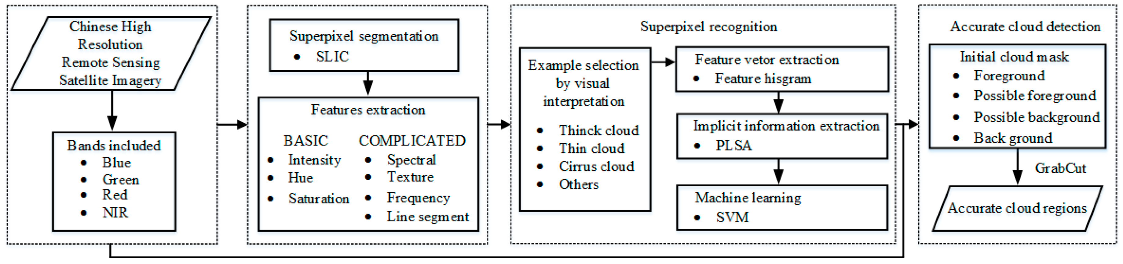
3. Methodology
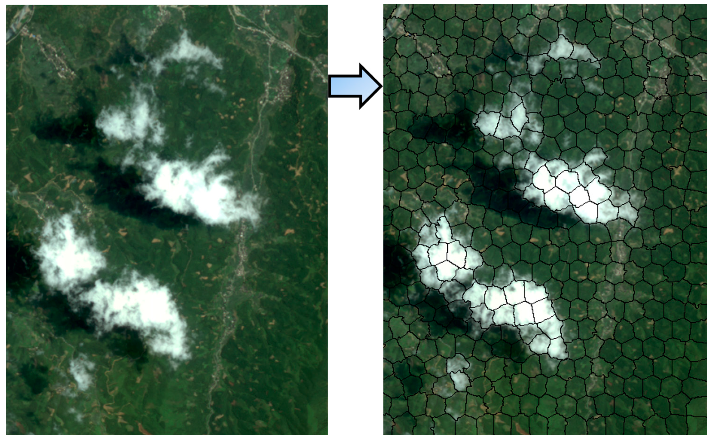
3.1. Superpixel Segmentation
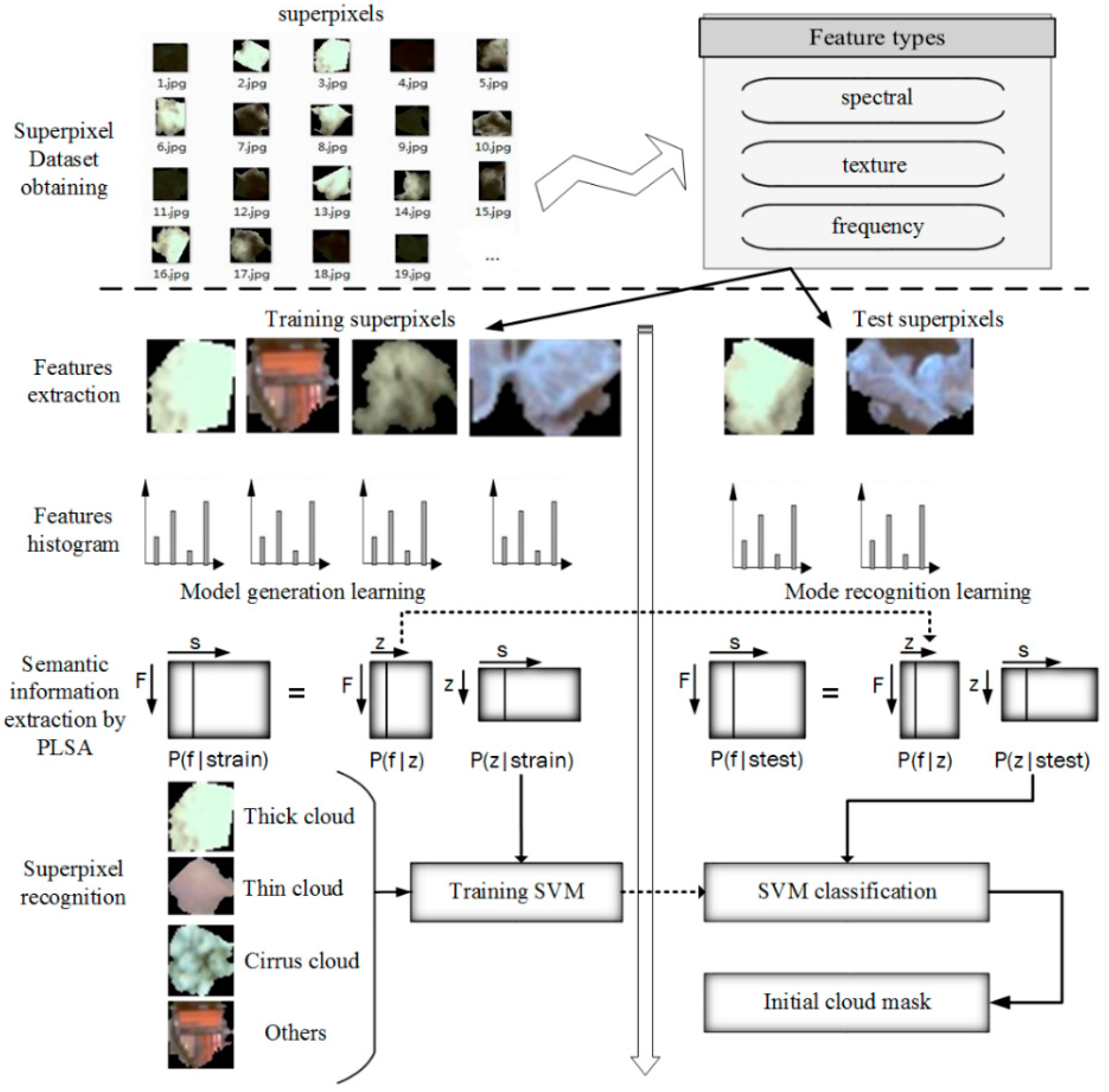
3.2. Superpixel Recognition
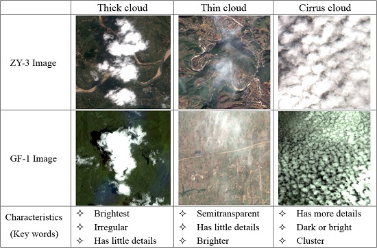
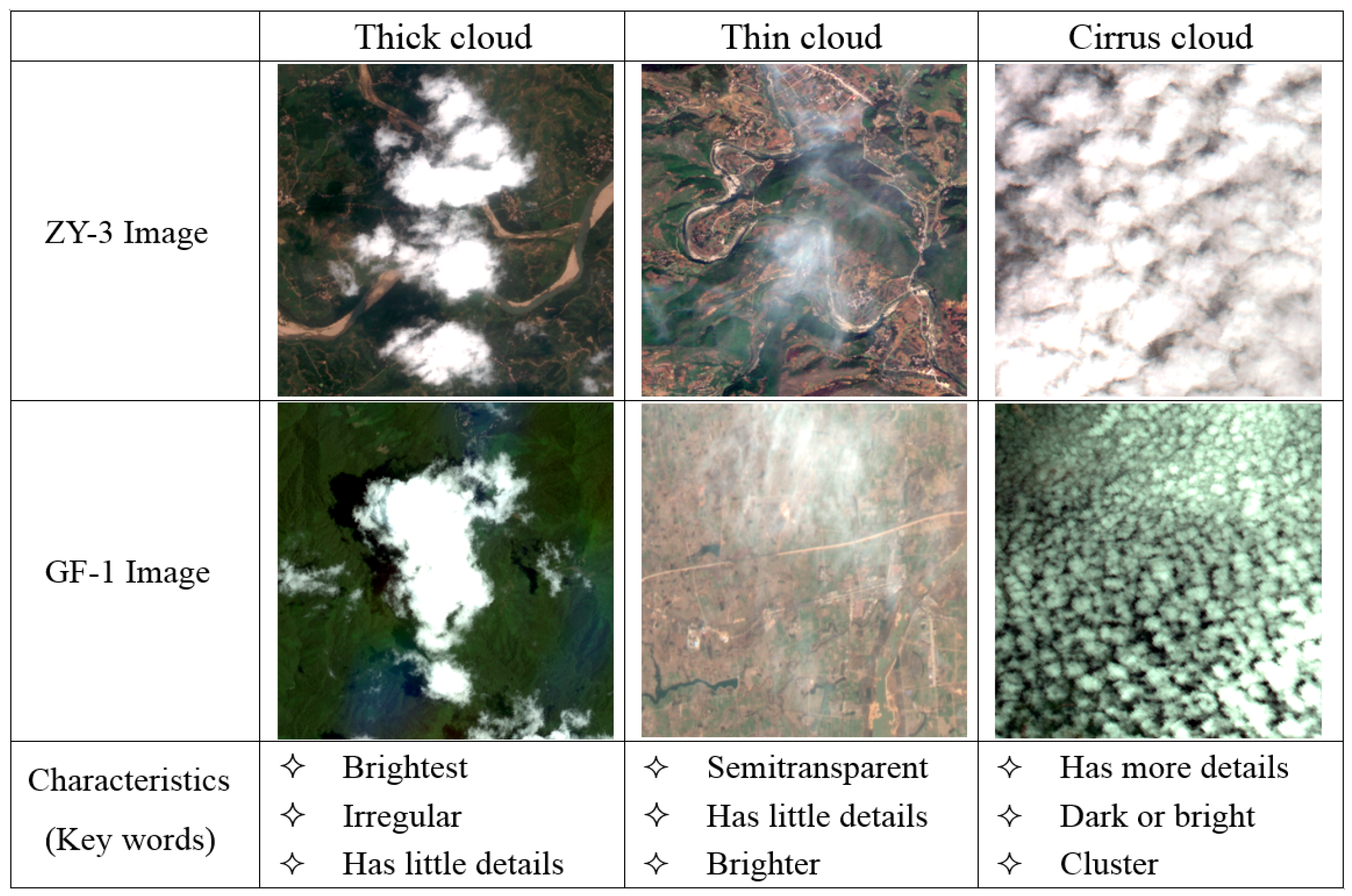
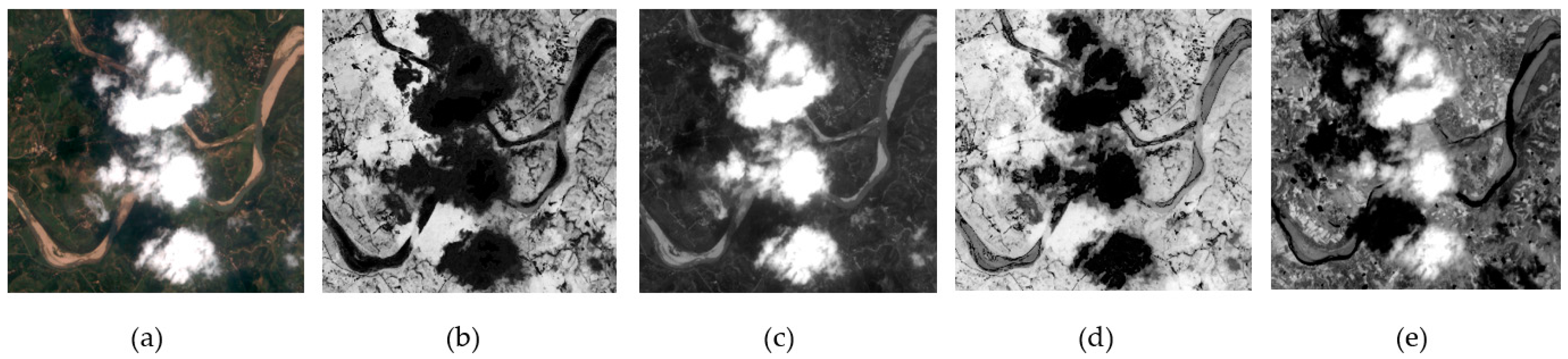
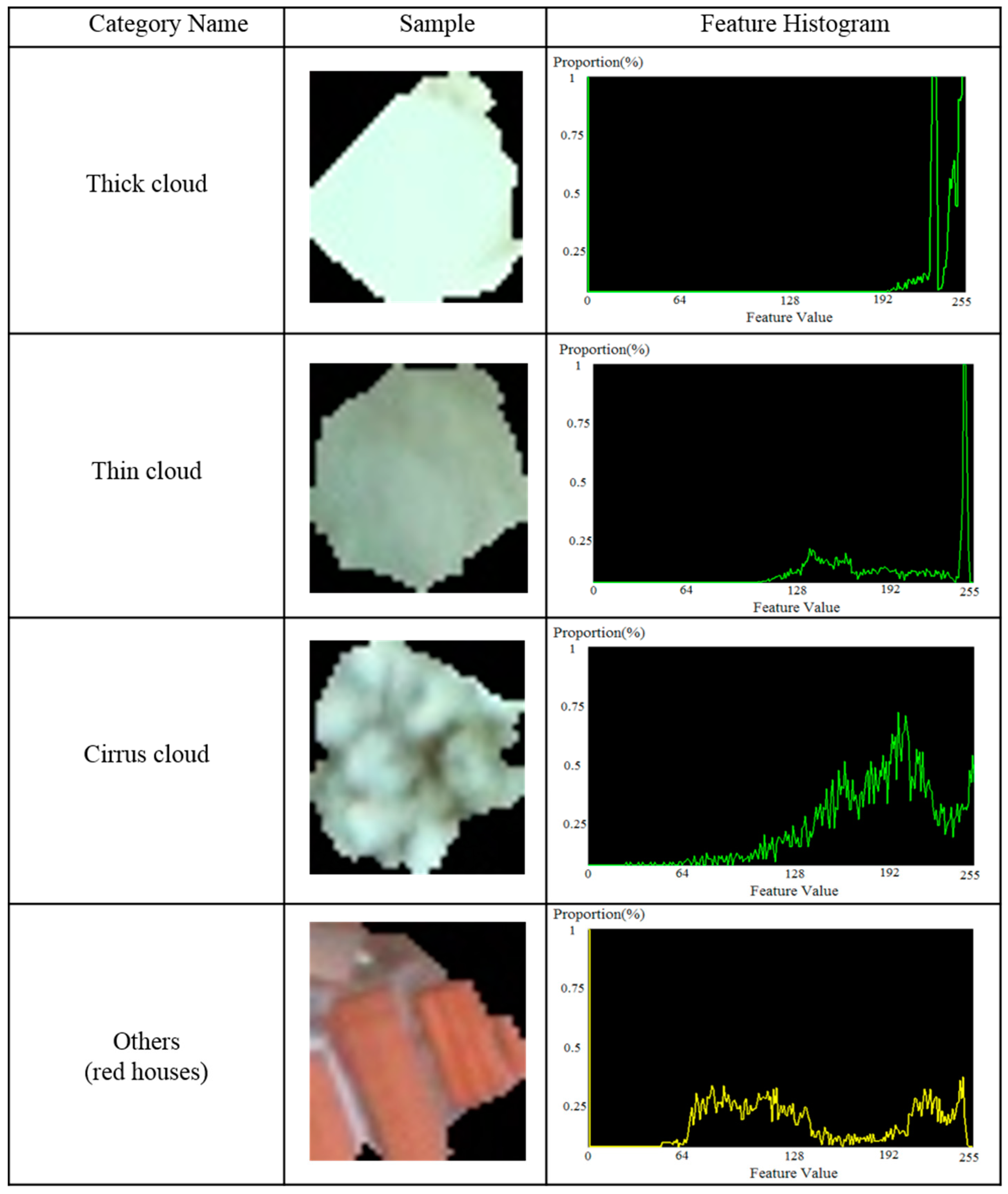
3.2.1. Features for Cloud Detection
- Most cloud regions often have lower hues than non-cloud regions
- Cloud regions generally have a higher intensity and NIR since the reflectivity of cloud regions is usually larger than that of non-cloud regions
- Cloud regions generally have lower saturation since they are white in a RGB color model
- The ground covered by a cloud veil usually has few details as the ground object features are all attenuated by clouds
- Cloud regions always appear in terms of clustering
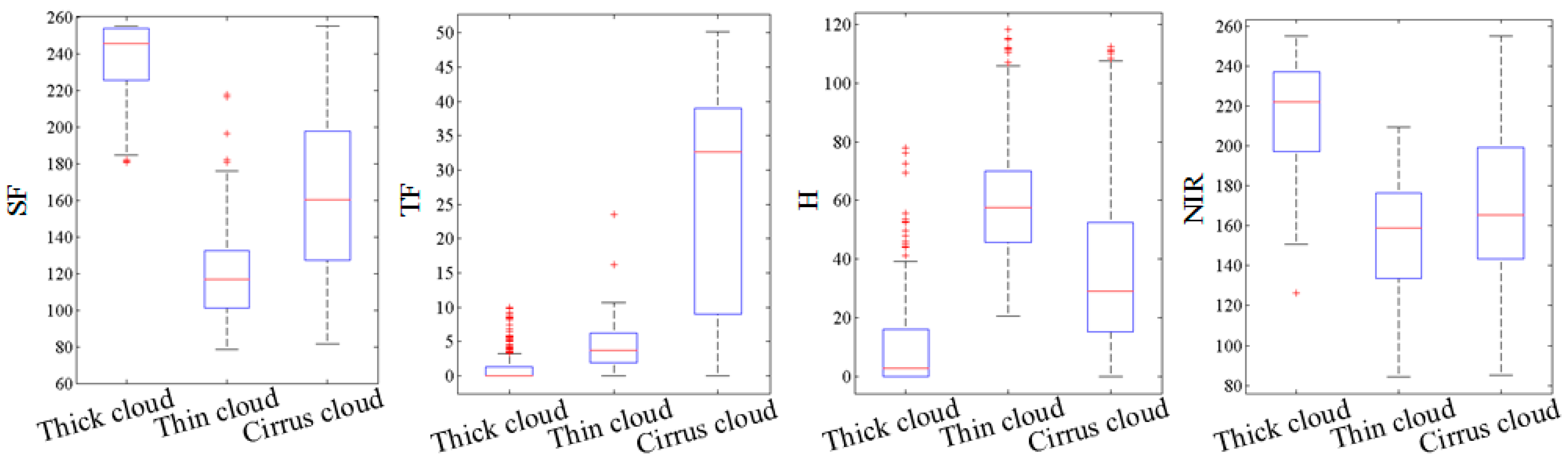
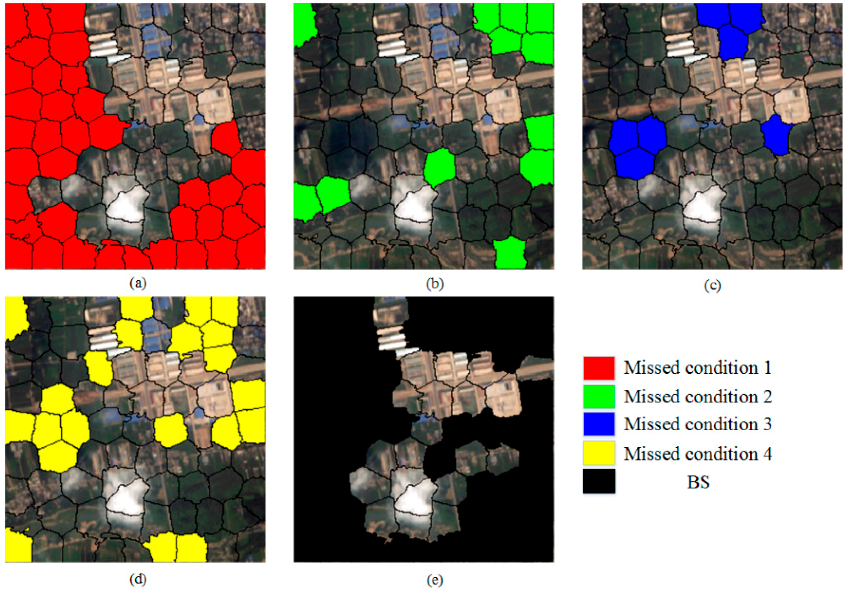
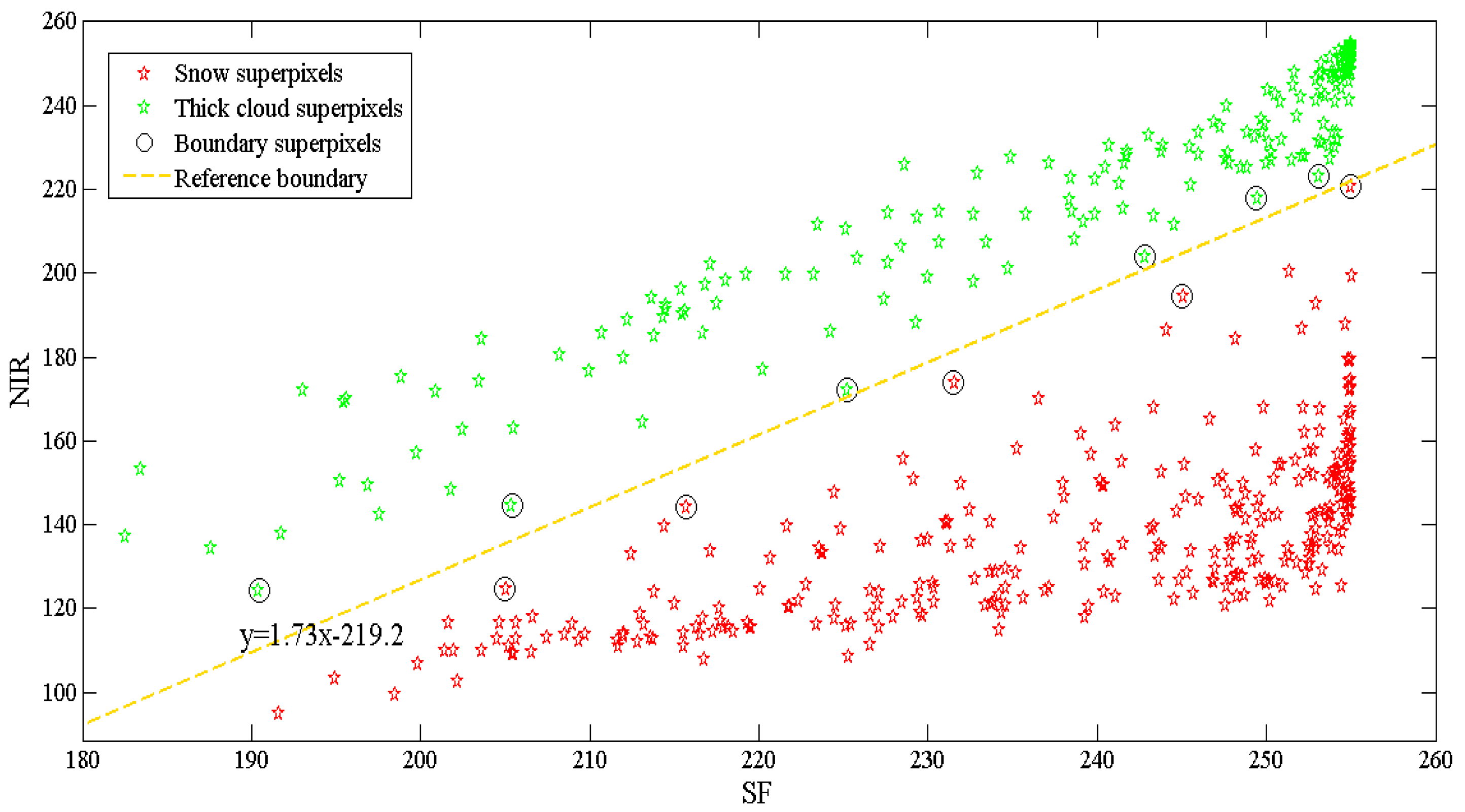
3.2.2. Background Superpixels (BS) Extraction
- Condition 1: The feature value of SF is larger than optimal threshold T;
- Condition 2: The feature value of TF is less than 50;
- Condition 3: The feature value of H is less than 120;
- Condition 4: The feature value of NIR is not less than 85.
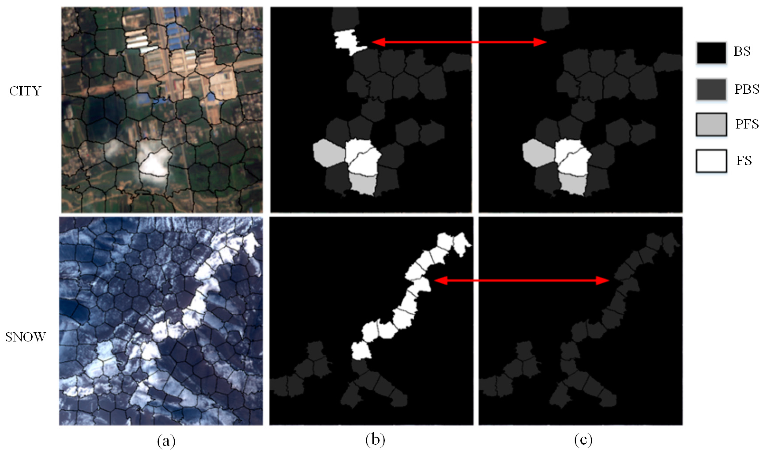
3.2.3. Cloud Mask Extraction
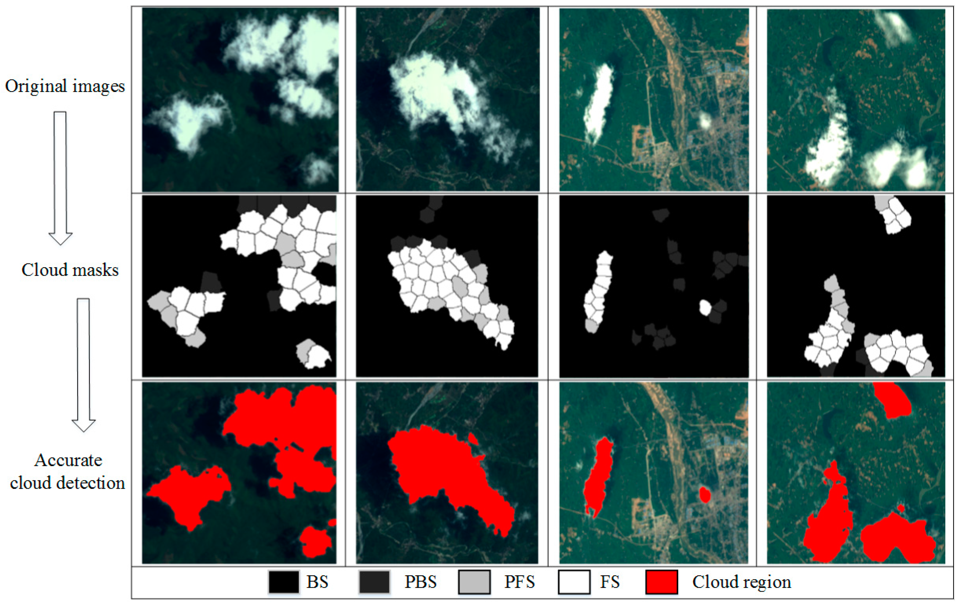
3.2.4. Accurate Cloud Detection
4. Method Feasibility Validation
4.1. Internal Feasibility Validation
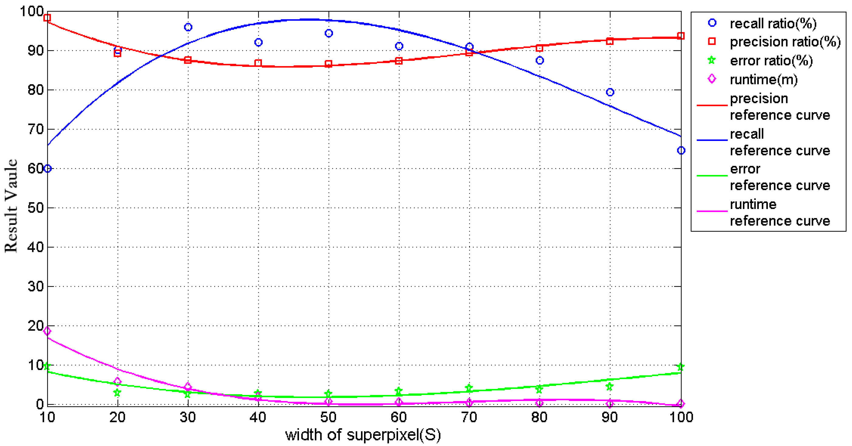
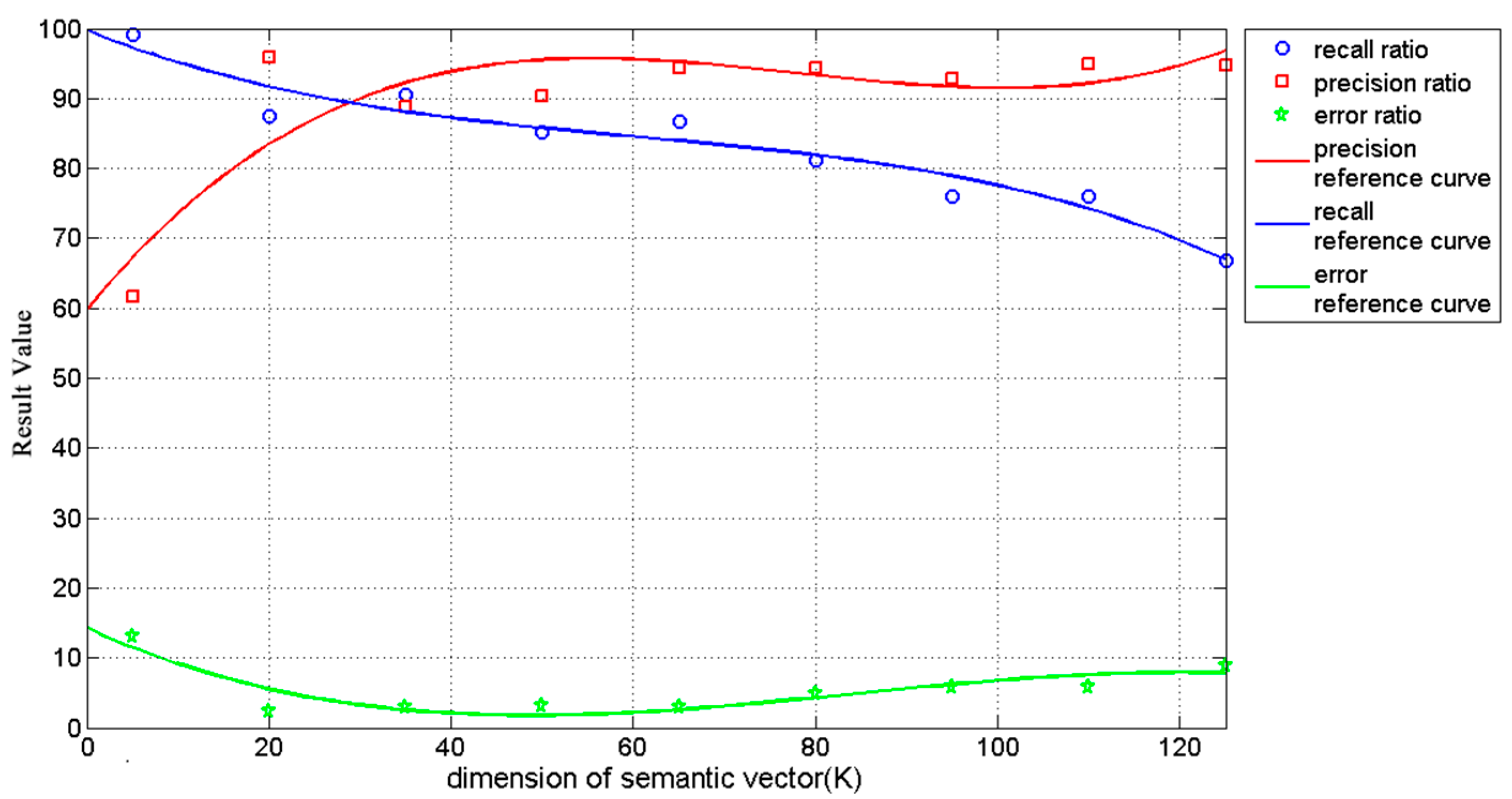
4.2. Parameters Sensitivity Validation
5. Experimental Results and Discussion
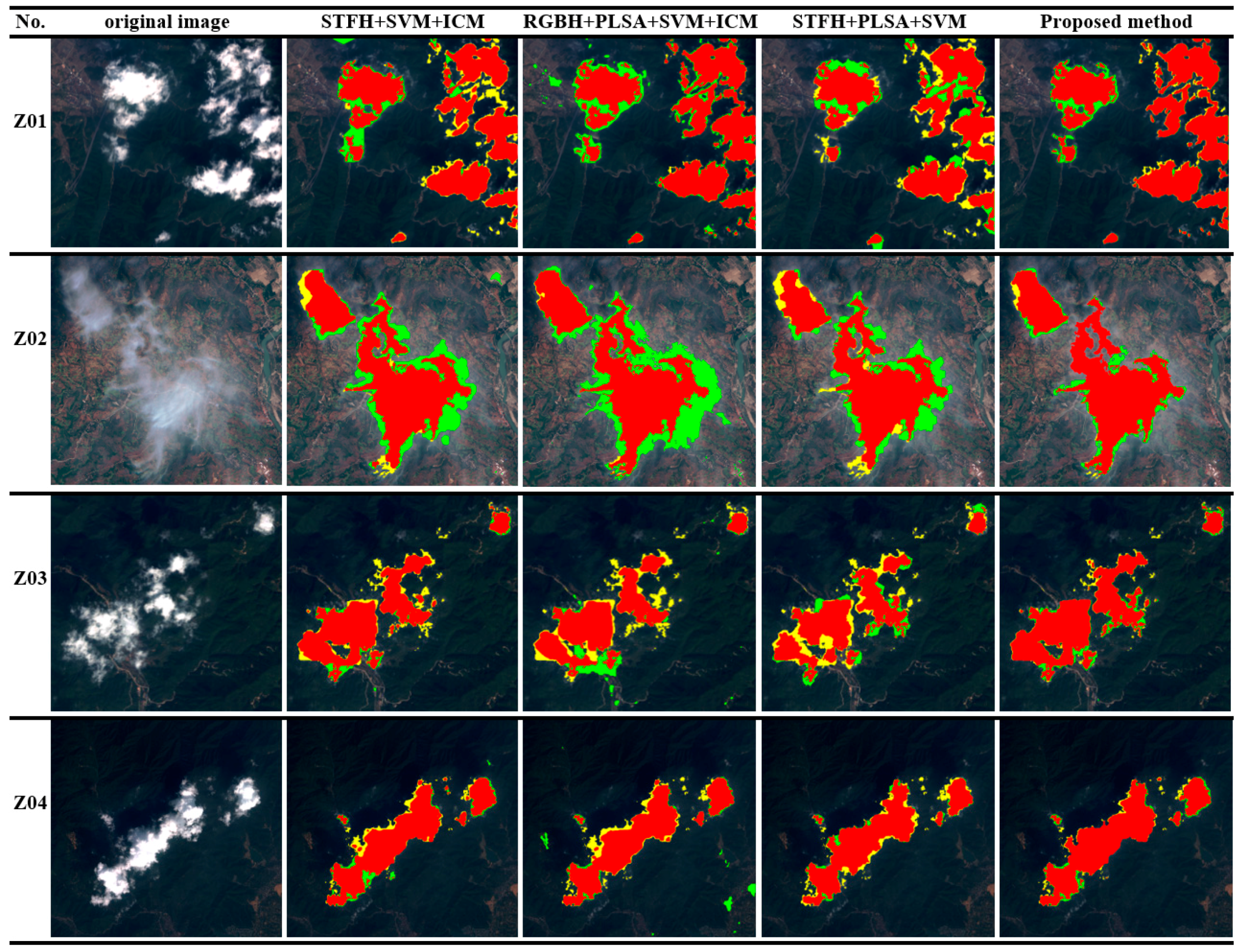
5.1. Case 1: Comparison with some Automatic Cloud Detection Algorithms
5.1.1. Methods and Results
5.1.2. Analysis and Discussion
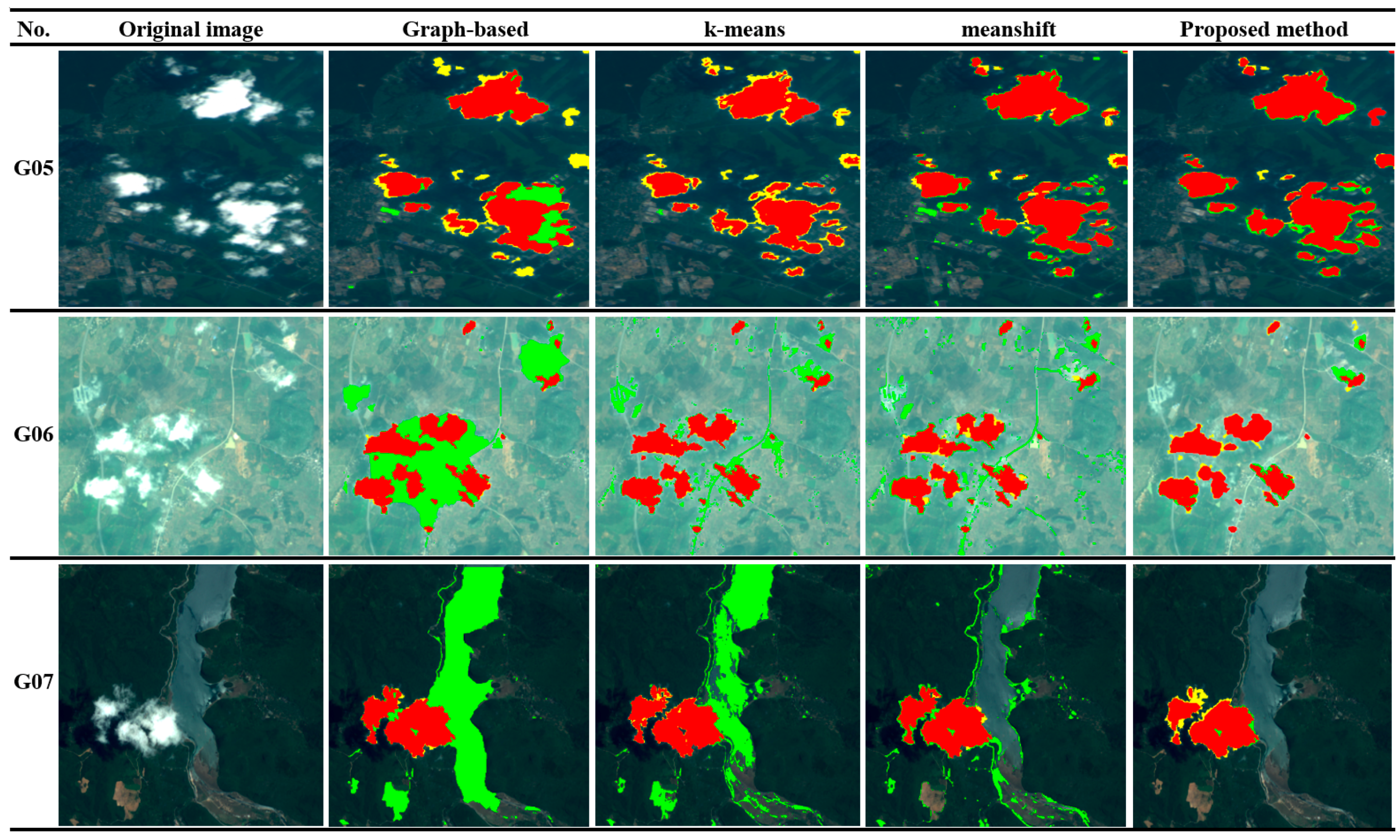
5.2. Case 2: Comparison with Some Automatic Image Segmentation Methods
5.2.1. Methods and Results
5.2.2. Analysis and Discussion
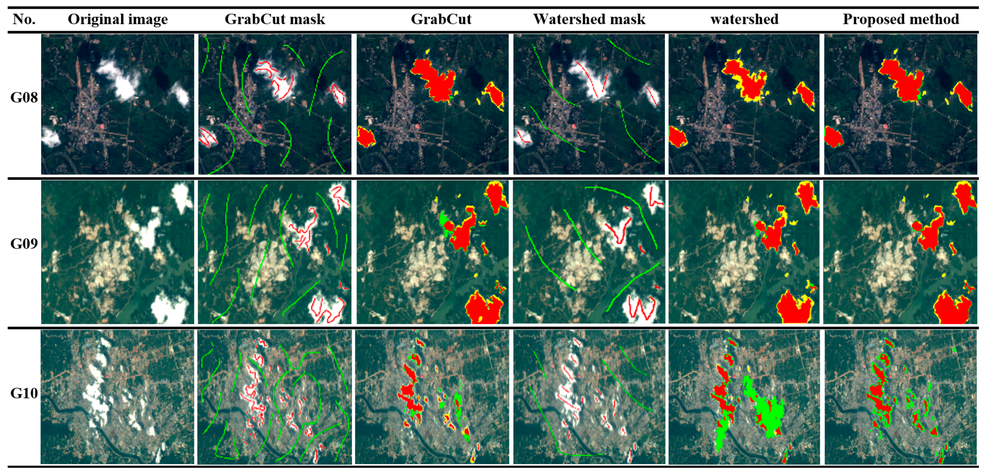
5.3. Case 3: Comparison with Some Interactive Image Segmentation Methods
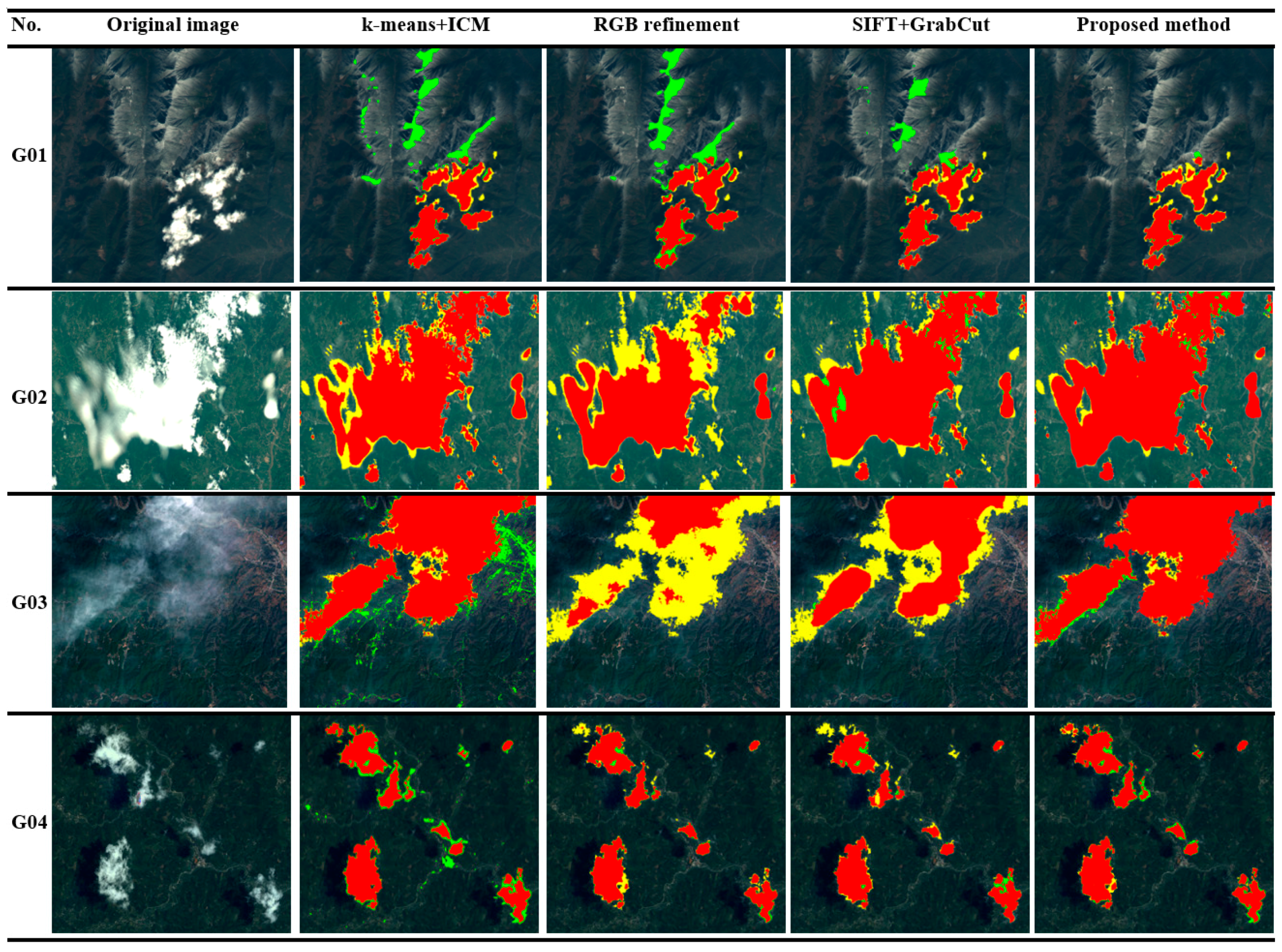
5.3.1. Methods and Results
5.3.2. Analysis and Discussion
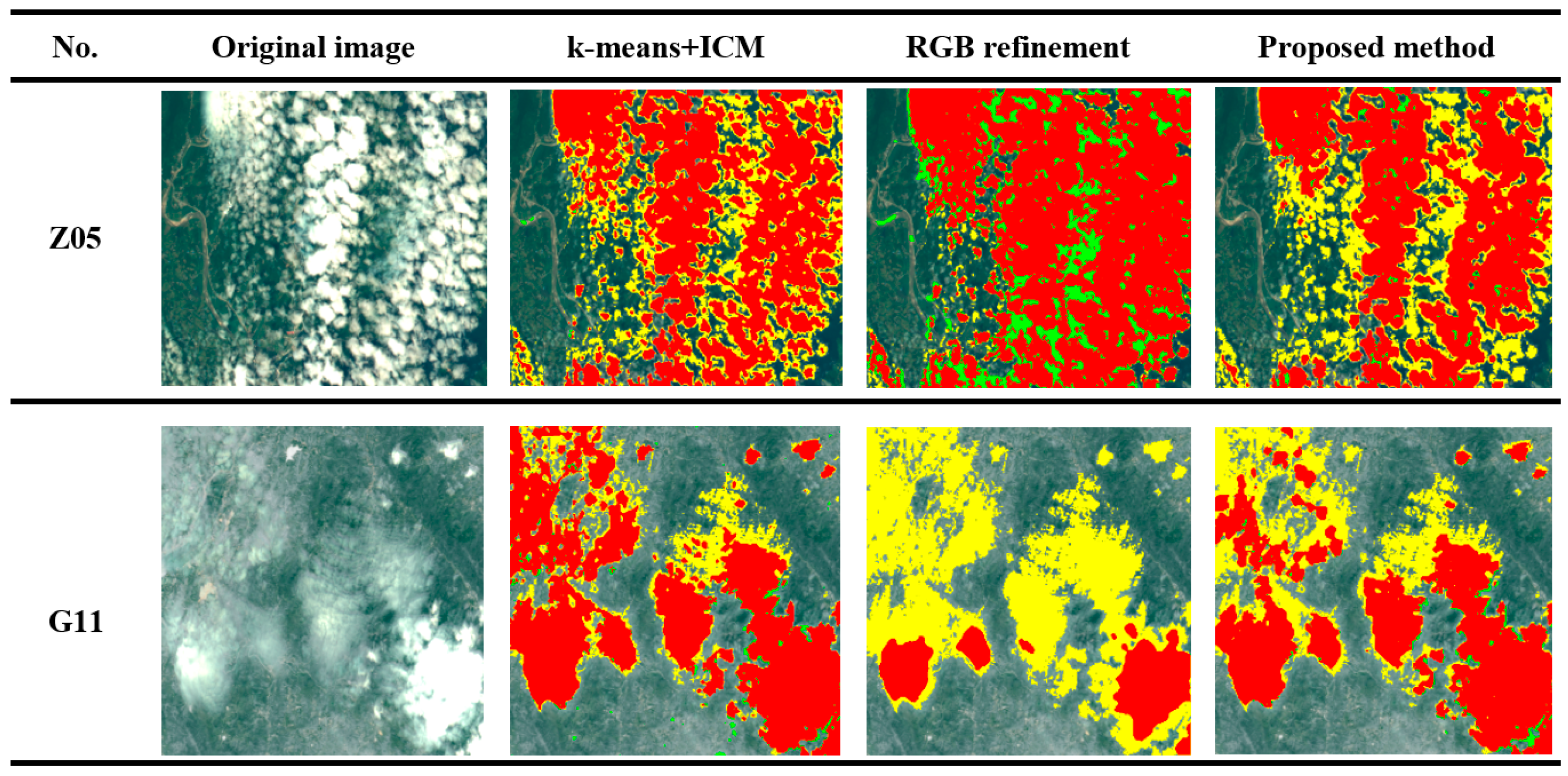
5.4. Algorithm Limitations
6. Conclusions
Acknowledgments
Author Contributions
Conflicts of Interest
Abbreviations
| PLSA | Probabilistic Latent Semantic Analysis |
| SLIC | Simple Linear Iterative Clustering |
| SVM | Support Vector Machine |
| GLCM | Gray-Level Co-occurrence Matrix |
| MRF | Markov Random Field |
| SPOTCASM | SPOT Cloud and Shadow Masking |
| HIS | Hue Intensity Saturation |
| SF | Spectral Feature |
| TF | Texture Feature |
| FF | Frequency Feature |
| LSF | Line Segment Feature |
| BS | Background Superpixels |
| PBS | Possible Background Superpixels |
| PFS | Possible Foreground Superpixels |
| FS | Foreground Superpixels |
| BOW | Bag-of-words |
| LSA | Latent Semantic Analysis |
| RBF | Radial Basis Function |
| GMM | Gaussian Mixture Model |
| ICM | Iterated Conditional Model |
References
- Zhang, Y.; Rossow, W.B.; Lacis, A.A. Calculation of radiative fluxes from the surface to top of atmosphere based on ISCCP and other global data sets. J. Geophys. Res. 2004, 109, 1121–1125. [Google Scholar] [CrossRef]
- Zhang, Y.J.; Wan, Y.; Wang, B. Automatic processing of Chinese GF-1 wide field of view images. In Proceedings of the 36th International Symposium on Remote Sensing Environment, Berlin, Germany, 11–15 May 2015.
- Chen, P.Y. An automated cloud detection method for daily NOAA-14 AVHRR data for Texas, USA. Int. J. Remote Sens. 2002, 23, 2939–2950. [Google Scholar] [CrossRef]
- Moustakidis, S.; Mallinis, G.; Koutsias, N. SVM-Based fuzzy decision trees for classification of high spatial resolution remote sensing images. IEEE Trans. Geosci. Remote Sens. 2012, 50, 149–169. [Google Scholar] [CrossRef]
- Zhu, Z.; Woodcock, C.E. Object-based cloud and cloud shadow detection in Landsat imagery. Remote Sens. Environ. 2012, 118, 83–94. [Google Scholar] [CrossRef]
- Hagolle, O.; Huc, M.; Pascual, D.V. A multi-temporal method for cloud detection, applied to FORMOSAT-2, VENµS, LANDSAT and SENTINEL-2 images. Remote Sens. Environ. 2010, 114, 1747–1755. [Google Scholar] [CrossRef] [Green Version]
- Gao, X.J.; Wan, Y.C.; Zheng, X.Y. Real-Time automatic cloud detection during the process of taking aerial photographs. Spectrosc. Spectr. Anal. 2014, 34, 1909–1913. [Google Scholar]
- Chylek, P.; Robinson, S.; Dubey, M K. Comparison of near-infrared and thermal infrared cloud phase detections. J. Geophys. Res. 2006, 111, 4763–4773. [Google Scholar] [CrossRef]
- Hong, G.; Zhang, Y. Wavelet-based image registration technique for high-resolution remote sensing images. Comput. Geosci. 2008, 34, 1708–1720. [Google Scholar] [CrossRef]
- Agüera, F.; Aguilar, F.J.; Aguilar, M.A. Using texture analysis to improve per-pixel classification of very high resolution images for mapping plastic greenhouses. ISPRS J. Photogramm. Remote Sens. 2008, 63, 635–646. [Google Scholar]
- Tran, D.B.; Puissant, A.; Badariotti, D. Optimizing spatial resolution of imagery for urban form detection—The cases of France and Vietnam. Remote Sens. 2011, 3, 2128–2147. [Google Scholar] [CrossRef]
- Huang, X.; Liu, X.; Zhang, L. A Multichannel Gray level co-occurrence matrix for multi/hyperspectral image texture representation. Remote Sens. 2014, 6, 8424–8445. [Google Scholar] [CrossRef]
- Ou, X.; Pan, W.; Xiao, P. In vivo skin capacitive imaging analysis by using grey level co-occurrence matrix (GLCM). Int. J. Pharm. 2014, 460, 28–32. [Google Scholar]
- Liu, J. Improvement of dynamic threshold value extraction technic in FY-2 cloud detection. J. Infrared Millim. Waves 2010, 29, 288–292. [Google Scholar]
- Huang, X.; Zhang, L. An SVM ensemble approach combining spectral, structural, and semantic features for the classification of high-resolution remotely sensed imagery. IEEE Trans. Geosci. Remote Sens. 2013, 51, 257–272. [Google Scholar] [CrossRef]
- Kaya, G.T. A hybrid model for Classification of remote sensing images with linear SVM and support vector selection and adaptation. IEEE J. Sel. Top. Appl. Earth Obs. Remote Sens. 2013, 6, 1988–1997. [Google Scholar] [CrossRef]
- Shao, P.; Shi, W.; He, P. Novel approach to unsupervised change detection based on a robust semi-supervised FCM clustering algorithm. Remote Sens. 2016, 8, 264. [Google Scholar] [CrossRef]
- Xu, X.; Guo, Y.; Wang, Z. Cloud image detection based on Markov Random Field. Chin. J. Electron. 2012, 29, 262–270. [Google Scholar] [CrossRef]
- Fisher, A. Cloud and Cloud-Shadow Detection in SPOT5 HRG imagery with automated morphological feature extraction. Remote Sens. 2013, 6, 776–800. [Google Scholar]
- Zhang, Y.; Guindon, G.; Li, X. A robust approach for object-based detection and radiometric characterization of cloud shadow using haze optimized transformation. IEEE Trans. Geosci. Remote Sens. 2014, 52, 5540–5547. [Google Scholar] [CrossRef]
- Hu, X.; Wang, Y.; Shan, J. Automatic recognition of cloud images by using visual saliency features. IEEE Geosci. Remote Sens. 2015, 12, 1760–1764. [Google Scholar]
- Zhang, Q.; Xiao, C. Cloud detection of RGB color aerial photographs by progressive refinement scheme. IEEE Trans. Geosci. Remote Sens. 2014, 52, 7264–7275. [Google Scholar] [CrossRef]
- Yuan, Y.; Hu, Y. Bag-of-Words and object-based classification for cloud extraction from satellite imagery. IEEE J. Sel. Top. Appl. Earth Obs. Remote Sens. 2015, 8, 4197–4205. [Google Scholar] [CrossRef]
- Zhang, Y.J.; Zheng, M.T.; Xiong, J.X. On-Orbit Geometric calibration of ZY-3 three-line array imagery with multistrip data sets. IEEE Trans. Geosic. Remote Sens. 2014, 52, 224–234. [Google Scholar] [CrossRef]
- Ren, X.; Malik, J. Learning a classification model for segmentation. In Proceedings of the 2003 Ninth IEEE International Conference on Computer Vision, Washington, DC, USA, 13–16 October 2003.
- Achanta, R.; Shaji, A.; Smith, K.; Lucchi, A.; Fua, P.; Süsstrunk, S. SLIC Superpixels; EPFL Technical Report 149300; École polytechnique fédérale de Lausanne: Lausanne, Switzerland, June 2010. [Google Scholar]
- Achanta, R.; Shaji, A.; Smith, K.; Lucchi, A.; Fua, P.; Süsstrunk, S. SLIC superpixels compared to state-of-the-art superpixel methods. IEEE Trans. Pattern Anal. Mach. Intell. 2012, 34, 2274–2282. [Google Scholar]
- Gioi, R.G.V.; Jakubowicz, J.; Morel, J.M.; Randall, G. LSD: A fast line segment detector with a false detection control. IEEE Trans. Pattern Anal. Mach. Intell. 2008, 32, 722–732. [Google Scholar]
- Liau, Y.T.; Liau, Y.T. Hierarchical segmentation framework for identifying natural vegetation: A case study of the Tehachapi Mountains, California. Remote Sens. 2014, 6, 7276–7302. [Google Scholar] [CrossRef]
- Hofmann, T. Unsupervised learning by probabilistic latent semantic analysis. Mach. Learn. 2001, 42, 177–196. [Google Scholar] [CrossRef]
- Huang, X.; Xie, C. Combining pixel- and object-based machine learning for identification of water-body types from urban high-resolution remote-sensing imagery. IEEE Trans. Geosci. Remote Sens. 2015, 8, 2097–2110. [Google Scholar] [CrossRef]
- Bishop, C.M. Pattern recognition and machine learning. J. Electron. Imaging 2006, 16, 140–155. [Google Scholar]
- Kanungo, T.; Mount, D.M.; Netanyahu, N.S. An efficient k-means clustering algorithm: Analysis and implementation. IEEE Trans. Pattern Anal. Mach. Intell. 2002, 24, 881–892. [Google Scholar] [CrossRef]
- Comaniciu, D.; Meer, P. Mean shift: A robust approach toward feature space analysis. IEEE Trans. Pattern Anal. Mach. Intell. 2002, 24, 603–619. [Google Scholar] [CrossRef]
- Felzenszwalb, P.F.; Huttenlocher, D.P. Efficient graph-based image segmentation. Int. J. Comput. Vis. 2004, 59, 167–181. [Google Scholar] [CrossRef]
- Rother, C.; Kolmogorov, V.; Blake, A. Grabcut: Interactive foreground extraction using iterated graph cuts. ACM Trans. Graph. 2004, 23, 309–314. [Google Scholar] [CrossRef]
- Zhang, M.; Zhang, L.; Cheng, H.D. A neutrosophic approach to image segmentation based on watershed method. Signal Process. 2012, 90, 1510–1517. [Google Scholar] [CrossRef]


| Algorithm | Published Year | Advantage | Disadvantage |
|---|---|---|---|
| k-means + ICM [18] | 2012 |
|
|
| SPOTCASM [19] | 2014 |
|
|
| Object-oriented [21] | 2015 |
|
|
| RGB refinement [22] | 2012 |
|
|
| SIFT + GrabCut [23] | 2015 |
|
|
| Satellite Parameters | ZY-3 | GF-1 | |
|---|---|---|---|
| Product Level | 1A | 1A | |
| Number of bands | 4 | 4 | |
| Wavelength (nm) | Blue: 450–520; Green: 520–590; Red: 630-690; NIR: 770–890 | ||
| Spatial resolution (m) | 5.8 | 8 | |
| Radiometric resolution | 1024 | 1024 | |
| Image size (pixel) | 8824 × 9307 | 4548 × 4596 | |
| Acquisition Time (year) | 2013 | 2013 | |
| Number of images | 36 | 42 | |
| Land cover types | Cloud types | Thin cloud, Thick cloud, Cirrus cloud | |
| Surface types | Forest, City, Sand, Bare land, River, Snow, etc. | ||
| Algorithm | Precision Ratio | Recall Ratio | Error Ratio | Runtime |
|---|---|---|---|---|
| Proposed method | 87.6% | 94.9% | 2.5% | 219 (s) |
| STFH + SVM + GrabCut | 89.0% | 82.8% | 5.7% | 107 (s) |
| RGBH + PLSA + SVM + GrabCut | 82.7% | 74.5% | 7.6% | 209 (s) |
| STFH + PLSA + SVM | 88.1% | 74.7% | 7.2% | 212 (s) |
| Algorithm | ER of G01 | ER of G02 | ER of G03 | ER of G04 |
|---|---|---|---|---|
| k-means + ICM | 3.8% | 7.4% | 6.0% | 3.1% |
| RGB refinement | 3.9% | 12.0% | 20.7% | 1.6% |
| SIFT + GrabCut | 2.7% | 6.0% | 10.5% | 1.6% |
| Proposed method | 1.5% | 3.3% | 2.4% | 1.7% |
| Algorithm | ER of G05 | ER of G06 | ER of G07 |
|---|---|---|---|
| Graph-based | 5.5% | 12.8% | 14.3% |
| k-means | 3.6% | 4.6% | 10.6% |
| meanshift | 3.4% | 5.0% | 4.0% |
| Proposed method | 2.8% | 1.7% | 1.1% |
| Algorithm | ER\WR of G08 | ER\WR of G09 | ER\WR of G10 | |||
|---|---|---|---|---|---|---|
| ER | WR | ER | WR | ER | WR | |
| GrabCut | 1.3% | 2.9% | 2.8% | 2.8% | 3.1% | 5.3% |
| Watershed | 2.4% | 1.2% | 3.3% | 2.9% | 6.6% | 1.6% |
| Proposed method | 1.5% | 0% | 2.4% | 0% | 2.3% | 0% |
| No. | Algorithm | Precision Ratio | Recall Ratio | Error Ratio |
|---|---|---|---|---|
| Z05 | Proposed method | 97.5% | 68.9% | 18.9% |
| k-means + ICM | 99.8% | 69.4% | 18.3% | |
| RGB refinement | 82.1% | 96.1% | 15.1% | |
| G11 | Proposed method | 96.8% | 62.7% | 17.9% |
| k-means + ICM | 97.1% | 78.5% | 12.6% | |
| RGB refinement | 99.9% | 20.5% | 36.6% |
© 2016 by the authors; licensee MDPI, Basel, Switzerland. This article is an open access article distributed under the terms and conditions of the Creative Commons Attribution (CC-BY) license (http://creativecommons.org/licenses/by/4.0/).
Share and Cite
Tan, K.; Zhang, Y.; Tong, X. Cloud Extraction from Chinese High Resolution Satellite Imagery by Probabilistic Latent Semantic Analysis and Object-Based Machine Learning. Remote Sens. 2016, 8, 963. https://doi.org/10.3390/rs8110963
Tan K, Zhang Y, Tong X. Cloud Extraction from Chinese High Resolution Satellite Imagery by Probabilistic Latent Semantic Analysis and Object-Based Machine Learning. Remote Sensing. 2016; 8(11):963. https://doi.org/10.3390/rs8110963
Chicago/Turabian StyleTan, Kai, Yongjun Zhang, and Xin Tong. 2016. "Cloud Extraction from Chinese High Resolution Satellite Imagery by Probabilistic Latent Semantic Analysis and Object-Based Machine Learning" Remote Sensing 8, no. 11: 963. https://doi.org/10.3390/rs8110963