Biomass Estimation Using 3D Data from Unmanned Aerial Vehicle Imagery in a Tropical Woodland

Abstract

Application of 3D data derived from images captured using unmanned aerial vehicles (UAVs) in forest biomass estimation has shown great potential in reducing costs and improving the estimates. However, such data have never been tested in miombo woodlands. UAV-based biomass estimation relies on the availability of reliable digital terrain models (DTMs). The main objective of this study was to evaluate application of 3D data derived from UAV imagery in biomass estimation and to compare impacts of DTMs generated based on different methods and parameter settings. Biomass was modeled using data acquired from 107 sample plots in a forest reserve in miombo woodlands of Malawi. The results indicated that there are no significant differences (p = 0.985) between tested DTMs except for that based on shuttle radar topography mission (SRTM). A model developed using unsupervised ground filtering based on a grid search approach, had the smallest root mean square error (RMSE) of 46.7% of a mean biomass value of 38.99 Mg·ha⁻¹. Amongst the independent variables, maximum canopy height (Hmax) was the most frequently selected. In addition, all models included spectral variables incorporating the three color bands red, green and blue. The study has demonstrated that UAV acquired image data can be used in biomass estimation in miombo woodlands using automatically generated DTMs.

1. Introduction

The Reducing Emissions from Deforestation and forest Degradation plus forest conservation, sustainable management of forest and enhancement of forest carbon stocks (REDD+) mechanism has given a financial incentive to developing countries for their efforts in reducing deforestation and forest degradation. According to requirements of the United Nations Framework Convention on Climate Change (UNFCCC), participating countries are supposed to report verified national level carbon estimates to benefit from the mechanism. Therefore, it is expected that each country implementing REDD+ should have a carbon monitoring system capable of collecting reliable data at designated time intervals using consistent methodologies.

Many countries rely on data captured through national forest inventories (NFIs) to estimate country level biomass and carbon stock estimates. The first step in a NFI involves developing a national land cover map displaying different forest strata across the country. Next, sample plot inventories are conducted on permanent sample plots distributed across the country. Allometric models are then applied to estimate average biomass and carbon stocks for sample plots lying within a given stratum. National level carbon stock is then estimated by applying the average biomass and carbon density values across the map with the same forest strata [1]. However, many developing countries, including Malawi, do not have comprehensive NFIs. Malawi is currently in the preparatory phase of implementing the REDD+ mechanism and a NFI is one of the planned activities [2,3].

In Malawi, miombo woodlands (Figure 1) constitute 92.4% of the country’s total forest area [4]. These woodlands are dominated by Brachystegia-Julbernardia-Isoberlinia species and they occur between 5° and 25° south of the equator in the upland plateau ecoregion of eastern and southern Africa within an altitude ranging from 600–4200 m. The region has a mean annual rainfall between 800 and 1400 mm [5]. In Malawi, a relatively small part of these woodlands are found in large continuous blocks, instead they are scattered over the landscape in 112 forest reserves as “islands” in cultivated land. The government of Malawi is targeting these forest reserves as potential REDD+ project areas. These forest reserves have variable sizes ranging between 42 and 114,780 ha [6]. Approximately 50% of the reserves may be characterized as small- to medium-sized (i.e., up to 2240 ha).

Ground-based forest inventories usually form a key component in NFIs. However, comprehensive ground-based inventories are associated with high labor and operational costs hence restrictive to most developing countries [7,8,9,10]. This has prompted researchers to search for other reliable but more cost effective biomass estimation methodologies. A promising approach aimed at reducing labor and operational costs, as well as improving the reliability of estimated biomass in NFIs, involve combining data from ground-based forest inventories and remote sensing [8,11,12,13,14].

For forestry applications, remotely sensed data are mainly sourced from three main systems, namely, airborne laser scanning (ALS), radio detection and ranging (RADAR) (e.g., synthetic aperture radar (SAR)) and optical images (e.g., satellite- or aerial images) [15,16]. Remote sensing has been widely applied in forestry for several decades in most countries, although with various degrees of success due to differences in data types, forest canopy cover, geographical and environmental conditions and methods used [16,17]. For example, estimation of forest biomass based on data from optical systems is usually challenged by clouds, shadows, saturation problems in forests with high biomass density, intra-crown spectral variance, low spectral variability and its two-dimensional (2D) nature [16,17]. RADAR systems are capable of improving biomass estimations due their ability to capture high quality three-dimensional (3D) data in all weather and light conditions. However, biomass estimation using such data is also affected by saturation problems in complex mature forest stands and also have difficulty in distinguishing vegetation types [16]. Data from ALS systems have shown great potential for forest biomass estimations in different forest types including boreal [18], temperate [19,20,21] and tropical forests [22,23] because ALS’s is able to overcome saturation problems better than other sensors when biomass density is ≥100 Mg·ha⁻¹ [14,15,16,24]. However, wide application of ALS data for large-scale forest biomass estimation has been limited due to high data acquisition costs.

On the other hand, application of unmanned aerial vehicles (UAVs) can enable acquisition of high quality 3D remotely sensed data for estimating forest biomass on small- to medium-sized forests wall-to-wall, or as a sampling tool in large forest areas, with relatively low costs [25,26,27,28,29]. Relatively little technical expertise is required for operating and acquiring images using UAVs, thus costs associated with hiring airborne image acquisition platforms are reduced. Furthermore, the availability of user-friendly structure from motion (SfM) and stereo-matching software that uses a photogrammetric approach to obtain 3D data reduces the need for hiring image processing services [26,27,30].

Results from recent research on small- to medium-sized boreal forests have demonstrated the potential of using UAVs for estimating forest biomass [27,31]. Application of this technology for REDD+ implementation in Malawi could be an attractive option since a substantial proportion of the potential project areas are small- to medium-sized forest reserves scattered across the country. However, the application of a UAV system for biomass estimation in tropical forests such as miombo woodlands first needs to be investigated because the forest structure in these woodlands is different from the boreal forests. Miombo woodlands are dry tropical forests dominated by relatively short trees with highly variable canopy structures [6,32,33] while boreal forests may have relatively tall trees with almost uniform sizes and shapes, few species and relatively simple canopy structures [34,35].

Several previous studies, including Mauya, et al. [36], Gregoire, et al. [37], Yang and Prince [38] and Fuller, et al. [39], among others, have attempted to estimate forest attributes in miombo woodlands using a combination of remote sensing and ground-based inventory data. Amongst the previous studies, Mauya, et al. [36] and Gregoire, et al. [37] are the only studies that utilized 3D ALS data. To the best of our knowledge, there are currently no studies in which 3D remotely sensed data captured by UAVs have been applied for biomass estimation in miombo woodlands.

Successful estimation of forest characteristics from 3D remotely sensed data is conditioned on the ability of the sensor to capture data also from the ground. Thus, the accuracy and precision of the final estimates of forest characteristics are a function of the quality of the digital terrain model (DTM). ALS sensors are generally well suited to collect point clouds describing the ground for generating a DTM even in dense forest areas. The photogrammetric approach can yield very dense point clouds in forested environments, but these data are mostly located in the top of the canopy.

When applying the photogrammetric approach, DTMs may be generated through a two-stage process. The first stage involves separating ground from vegetation points (ground filtering). In the second stage, the data from the ground points are interpolated to estimate ground elevation at places where there are no data to get a continuous ground surface [40].

Most studies utilizing the UAVs technology utilize DTMs derived from ALS data because they are regarded as most accurate and reliable [27,41]. However, due to the high costs associated with acquiring ALS data, it is imperative to utilize UAVs in developing countries to search for alternative and cost efficient DTM generating approaches. Furthermore, several algorithms for DTM generation are available including Terrascan [42] and Fusion [43]. Most of these algorithms can be parameterized in different ways. Thus, the main objective of this study was to evaluate application of 3D data derived from UAV imagery in biomass estimation and to compare impacts of DTMs generated from different methods and parameter settings.

2. Materials and Methods

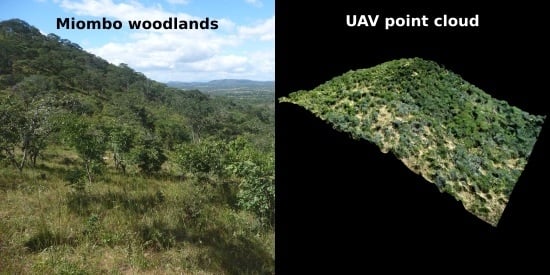
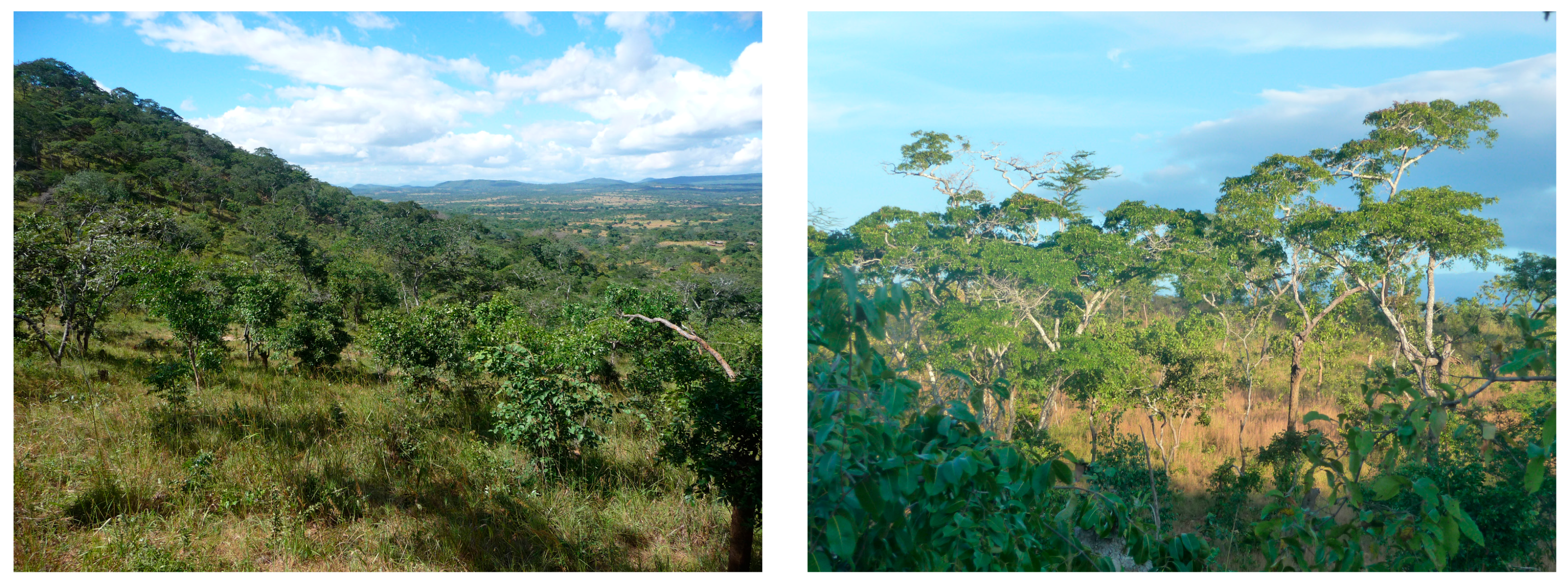
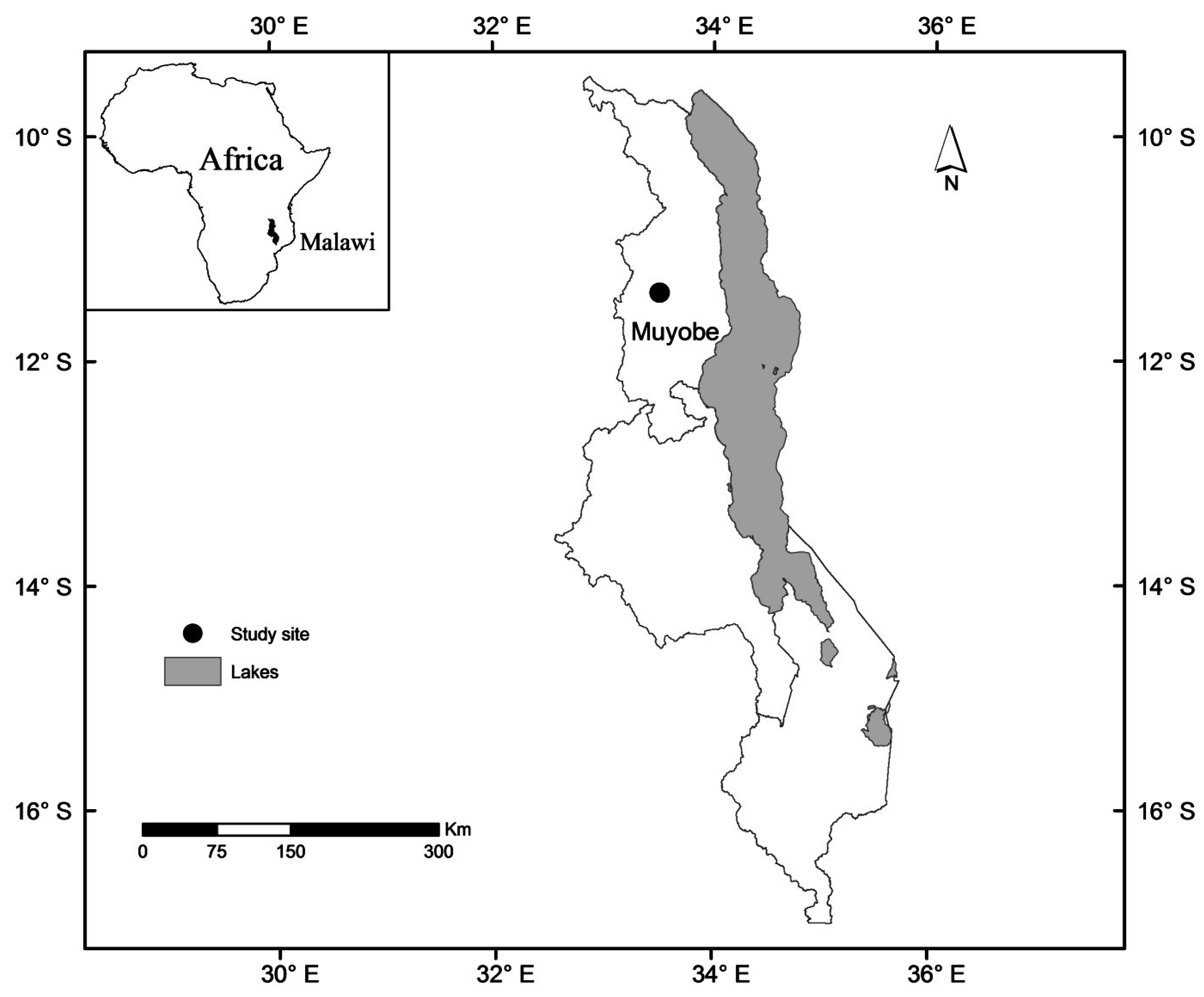
2.1. Study Area

The study was conducted in Muyobe community forest reserve (11°35′S, 33°65′E, 1169–1413 m above sea level), located in Mpherembe traditional authority in Mzimba district in the northern region of Malawi (Figure 2). This forest reserve was established in 2000 to save it from rampant deforestation happening in and around the area due to tobacco farming. The forest reserve is now managed through a committee whose members are representatives from all villages surrounding the forest. The forest reserve is 486 ha, which is a common size for many small- to medium-sized forest reserves in Malawi. Ferrosols are the dominant soil type in the study area [44]. For the period 1975–2005, the mean annual rainfall was 889 ± 146 mm and the mean annual daily minimum and maximum temperatures were 15 ± 1.6 °C and 26 ± 0.6 °C, respectively (the nearest weather station is located about 69 km south of the study area). The rain season lasts from December to April. The study area comprises miombo woodlands with Julbernadia globiflora, Diplorhychus condylocarpon and Combretum zeyheri as dominant species.

2.2. Data Collection

2.2.1. Sampling Design and Ground Reference Data Collection

Ground reference biomass was based on data from a forest inventory conducted on 107 systematically distributed circular sample plots (radius = 17.84 m, 0.1 ha) for 15 days from 25 April to 10 May 2015. Precise registration of the positions of centers for sample plots is very important in remote sensing-assisted forest inventories. In this study, positions of the plot centers were measured with a differential Global Navigation Satellite Systems (dGNSS) unit. The dGNSS unit is comprised of two Topcon legacy- E +40 dual frequency receivers. One of the receivers was used as base station unit and the other as a rover field unit. The receivers observe pseudo-range and carrier phase of both the American Global Positioning System (GPS) and the Russian Global Navigation Satellite System (GLONASS) to provide precise location. During the study, the baseline between the base station and the rover unit was approximately 25 km. The position of the base station was determined using Precise Point Positioning (PPP) with GPS and GLONASS data collected continuously for 24 h as suggested by Kouba [45]. The rover field unit at the plot centers was placed on a 2.98 m rod for an average of 33 ± 20 min using a one-second logging rate. The recorded plot center coordinates were post-processed using the RTKLIB software [46] and the results revealed that the maximum deviations for northing, easting and height were 1.16 cm, 3.02 cm and 3.06 cm, respectively.

On each plot, the following tree variables were recorded: diameter at breast height (dbh) (using a caliper or a diameter tape), and scientific name of all trees with dbh ≥ 5 cm. Furthermore, total tree height (ht) of up to 10 randomly selected sample trees within each plot were measured using a Vertex hypsometer.

For each tree in respective sample plots, we calculated biomass by using a model developed by Kachamba, et al. [47] with dbh and ht as independent variables:

$$Biomass=0.103685\times db{h}^{1.921719}\times h{t}^{0.844561}$$

(1)

Before calculating biomass, we predicted the ht of trees whose heights were not measured in the respective sample plots using a height-diameter model developed from the sample trees from all sample plots:

$$ht=1.3+\text{exp}\left(3.75876-6.01583\times db{h}^{-0.42991}\right)$$

(2)

The performance criteria for the ht model were as follows: pseudo-R² of 0.65, root mean square error (RMSE) of 1.9 m and a mean prediction error (MPE) of 0.1 m.

The pseudo-R² was calculated as:

$${\text{pseudo-R}}^2=1-(\frac{SSR}{CSST})$$

(3)

where SSR is the sum of squared residuals and CSST is the corrected total sum of squares. The RMSE and MPE were calculated as:

$$\text{RMSE}=\sqrt{\frac{{\sum }_{\mathrm{i}=1}^{\mathrm{n}}{\left(y_i-{\widehat{y}}_i\right)}^2}{n}}$$

(4)

$$\text{MPE}=\frac{{\sum }_{i=1}^n\left(y_i-{\widehat{y}}_i\right)}{n}$$

(5)

where $y_i$ is the ground reference biomass for plot i and ${\widehat{y}}_i$ is the predicted biomass for plot i, respectively, and n is the number of sample plots. Biomass (Mg.ha⁻¹), basal area (m²·ha⁻¹) and number of stems (ha⁻¹) of the respective sample plots were calculated by summation of the individual tree biomass and basal area values and the number of stems, within a given plot and scaling them to per hectare values by plot area. The mean height of trees for each plot was calculated as Lorey’s mean height, i.e., mean height weighted by basal area of individual trees. The ground reference values are presented in

Table 1. Ground reference values for the sample plots.

Characteristic	Ground Reference Values
	Range	Mean	Std 1	Cv 2	Stderr 3
Biomass (Mg·ha−1)	0–125.59	38.99	29.49	75.62	2.85
Basal area (m2·ha−1)	0–16.10	5.32	3.78	71.06	0.37
Number of stems (ha−1)	0–830	337	178	53	17
Lorey’s mean height (m)	3.76–14.58	8.81	2.41	27.31	0.23

¹ Std = Standard deviation, ² Cv = Coefficient of variation, ³ Stderr = Standard error.

.

2.2.2. UAV Imagery Collection

The UAV images were acquired during four days from 23 to 26 April 2015. At this time of the year, the rain had just stopped and trees still had leaves on them. Due to time constraints, the images had to be acquired over the entire day, i.e., morning, noon and evening. This will also be the case in an operational setting. Therefore, differences in shadow effects were expected in the acquired images. The images were acquired using a SenseFly eBee fixed-wing UAV [48] equipped with a Canon IXUS127 HS Digital camera. The dimensions and weight of camera with battery and memory card were 93.2 mm × 57.0 mm × 20.0 mm and 135 g, respectively. The camera produces 16.1 megapixel images in the red, green and blue spectral bands. The camera automatically set with a shutter speed of 1/2000 s. The eBee is made from flexible foam and the weight is 537 g without camera. The eBee is also equipped with an inertial measurement unit as well as an on-board Global Navigation Satellite Systems (GNSS) to control the flight and to provide a rough positioning [48].

Prior to taking images, positions of ground control points (GCPs) as well as landing and takeoff points, e.g., on open areas with no trees within the forest and agricultural fields near the forest, were identified and measured. The GCPs were made of a set of 1 m × 1 m cross-shaped timber planks painted white and some black and white 50 cm × 50 cm checkerboards. The position of the center of each GCP was measured using the same procedure as used when locating plot centers for the sample plot inventory described above. The data were collected for an average of 13 ± 6 min for each GCP with a 1-s logging rate. The recorded coordinates for each GCP were post-processed similarly as the sample plots. The results from the RTKLIB software revealed that maximum deviations for northing, easting and height were 2.24 cm, 4.50 cm and 4.46 cm, respectively.

Acquisition of images was controlled from a laptop computer with a mission control software called eMotion 2 version 2.4 [48]. All the flights were planned in the mission control software prior to flying. For navigation purposes, we used a georeferenced base map from Microsoft Bing maps covering the study area. For this study we applied end and side image overlaps of 80% and 90%, respectively, as well as a flight height above the ground of 325 m. Finally, images covering the entire forest were taken in all the designated strips. A summary of flight characteristics for each flight day is presented in

Table 2. Summary of flight characteristics for each flight block of imagery collection.

Date	Number of Flights	Number of Images	Flight Time (min)	Wind Speed (m·s−1)	Cloud Cover (%)
23 April 2015	8	1241	153	6.0–9.5	10–80
24 April 2015	7	1301	146	6.0–9.0	20–80
25 April 2015	6	1118	132	5.0–9.0	10–100
26 April 2015	1	273	26	3.0–4.0	50

.

2.3. Image Processing

Agisoft Photoscan Professional version 1.1 [49] was used to generate a 3D point cloud from the acquired images. This software uses both SfM and stereo-matching algorithms for image alignment and multi-view stereo reconstruction. The process for generating a 3D point cloud involved: (a) image alignment using the inbuilt SfM algorithms; (b) mesh building; (c) guided marker positioning and optimization of camera alignment (georeferencing of created scene) where the guided marker positioning involved importing coordinates for the GCPs and manually refining the estimated positions of the GCPs so as to improve camera orientation and position estimates (since the GNSS onboard the SenseFly eBee provide rough positioning); and (d) building the dense point cloud. Parameter settings for the processes in (a)–(d) are displayed in

Table 3. Processing steps with corresponding parameter settings in Agisoft Photoscan Professional software for generation of 3D point cloud from UAV imagery.

Task	Parameters
(a) Image alignment	Accuracy: high
	Pair selection: reference
	Key points: 40,000
	Tie points: 1000
(b) Mesh building	Surface type: height field
	Source data: dense cloud
	Face count: high
(c) Guided marker positioning	Manual positioning of markers on the 14 GCPs for all the photos where a GCP was visible
(d) Building dense point cloud	Quality: medium
	Depth filtering: mild

. All parameters were chosen based on empirical experience in Puliti, et al. [27]. Finally, we added spectral information from the imagery, i.e., red, green and blue image bands, to the point cloud. According to Wallace, et al. [29], spectral information from a UAV point cloud can present additional useful information for estimating other non-structural properties of the canopy.

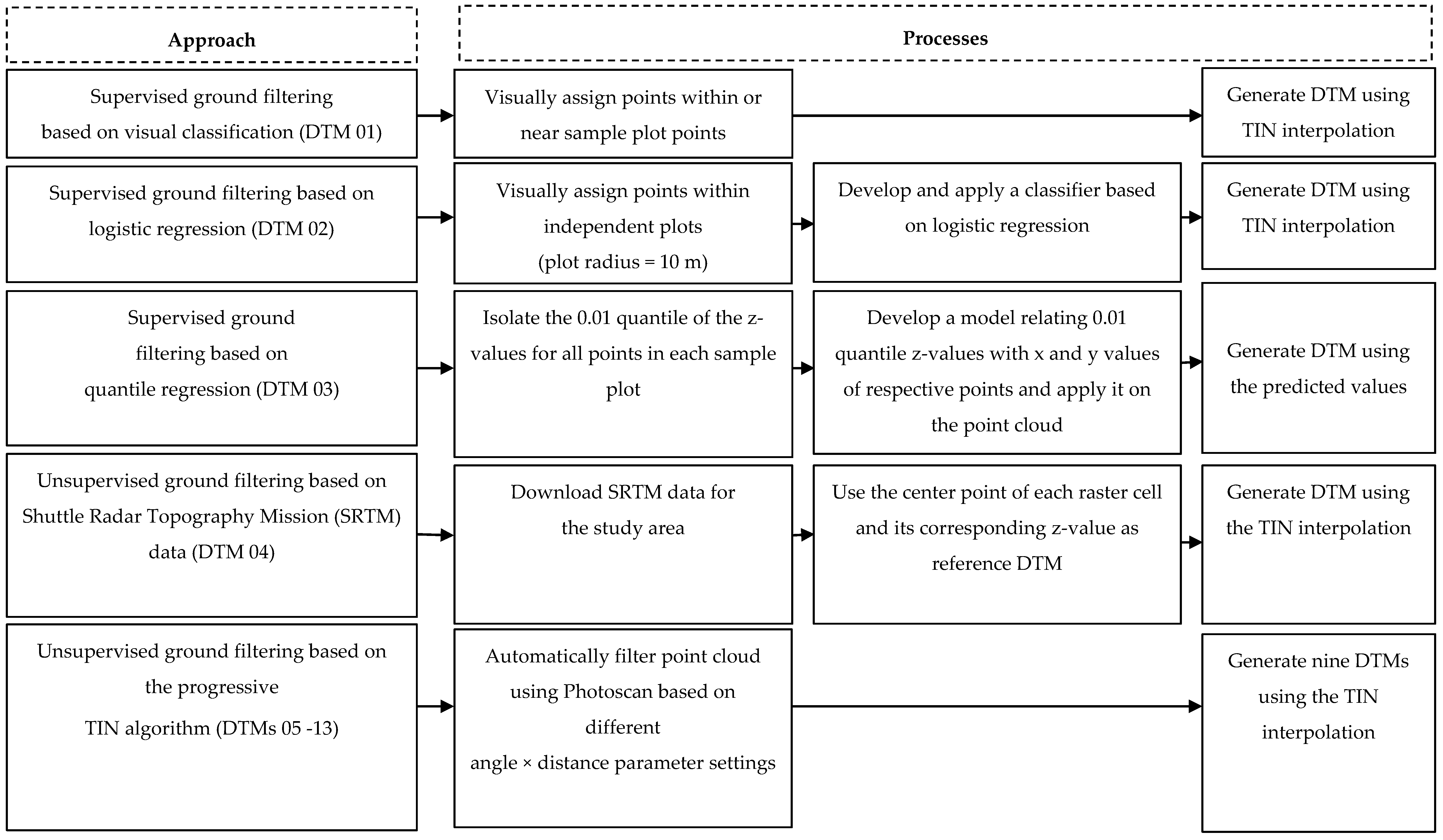
2.4. DTM Generation Methods

Five different approaches, with a total of 13 variants for generating DTMs, were tested (Figure 3): (a) supervised ground filtering based on visual classification; (b) supervised ground filtering based on logistic regression; (c) supervised ground filtering based on quantile regression; (d) unsupervised ground filtering based on shuttle radar topography mission (SRTM); and (e) unsupervised ground filtering based on the progressive triangular irregular network (TIN) algorithm.

2.4.1. Supervised Ground Filtering Based on Visual Classification

The first step involved producing an orthophoto for the entire area to guide the visual identification of areas with and without vegetation. Points, within and around all the sample plots, were then visually assigned to either ground or non-ground classes depending on whether they fell on an area with or without vegetation. The ground-class points were then used to create DTM as a TIN surface. This DTM was denoted as DTM 01 for further analysis. The DTM was finally used to calculate the height relative to the ground for all points by subtracting respective TIN values from each point.

2.4.2. Supervised Ground Filtering Based on Logistic Regression

In order to filter the respective point clouds, a supervised ground filtering approach with a standard binary logistic regression classifier was applied [50]. To train the model, visual classification was carried out on 132 circular areas of size 314 m² (radius 10 m) located with a systematic offset of 110 m in north and east from the sample plots. From a total of 495,457 points, approximately 23% were classified as ground points. The following logistic regression model was then fitted:

$$ln\left(\frac{P_j}{1-P_j}\right)={\beta }_0+{\beta }_1{R}_j+{\beta }_2{G}_j+{\beta }_3{B}_j+{\epsilon }_j$$

(6)

where P_j is the probability of point j being a ground point; R, G and B are the red, green and blue spectral information in each point, respectively; β₀, β₁ and β₂ are regression coefficients; and ε_ij is the random error component.

All identified ground points were then used to generate a DTM and calculate the height relative to the ground for all points using the approach described in Section 2.4.1. This DTM was denoted as DTM 02 for further analysis.

2.4.3. Supervised Ground Filtering Based on Quantile Regression

Quantile regression enable fitting of regression curves to other parts of the distribution of the response variable than the mean [51,52]. An assumption was made that the points representing the 0.01 quantile of the height-values of each sample plot could be considered ground heights. The relationship between the height-values against the easting and northing values of each point (j) at the sample plot (i) was then modeled as follows:

$$z_{ij}={\beta }_0+{\beta }_1{x}_{ij}+{\beta }_2{y}_{ij}+{\epsilon }_{ij}$$

(7)

where (z_ij) is the height-value; β₀, β₁ and β₂ are regression coefficients; x_ij is the easting; y_ij is the northing; and ε_ij is the random error component. The fitted height-values (${\widehat{z}}_{ij}$) of the regression model were then used to calculate the height relative to the ground for all points in a given plot. This ground classification was denoted as DTM 03 for further analysis.

2.4.4. Unsupervised Ground Filtering Based on Shuttle Radar Topography Mission (SRTM).

In remote areas of the earth as well as in developing countries, the best source of terrain heights are usually based on the SRTM [53]. In this study, the center points in the SRTM pixels and the corresponding height value were used to create a TIN surface. The DTM was denoted as DTM 04 for further analysis. The DTM was finally used to calculate the height relative to the ground for all points in a given plot using the approach described in Section 2.4.1.

2.4.5. Unsupervised Ground Filtering Based on the Progressive TIN Algorithm

A standard method for classifying ground points in point cloud data is based on the principles of the progressive TIN algorithm developed by Axelsson [54]. A variant of this algorithm is implemented in Agisoft Photoscan software [49]. The algorithm divides the point cloud into cells of a certain size. In this study, a cell size of 50 m was applied. In each cell, the lowest point is detected, and then triangulated to produce a first approximate terrain model. Next, parameters describing the angle between a point and the DTM surface and the maximum distance between a point and the DTM surface are set. In this study a grid search approach was applied to test different values for maximum distance and angle parameters. Based on the preliminary tests, the following angle–distance parameter combinations were chosen for further testing: 3-1, 3-3, 3-6, 6-1, 6-3, 6-6, 9-1, 9-3 and 9-6. For each of these combinations, a DTM was generated as a TIN surface of the points classified as ground. For further analysis, the DTMs were denoted as DTM 05–13, respectively. The DTMs were finally used to calculate the height relative to the ground for all points using the approach described in Section 2.4.1.

2.5. Variable Extraction

For each of the generated DTMs, variables describing plot-level canopy height and canopy density were then extracted as described by Næsset [55]. Variables describing canopy height included maximum and mean values (Hmax, Hmean), standard deviation (Hsd), coefficient of variation (Hcv), kurtosis (Hkurt), skewness (Hskewness) and percentiles at 10% intervals (H₁₀, H₂₀,…, H₉₀). A height threshold of 0.5 m was applied in order to separate trees from low vegetation. Furthermore, canopy density variables were derived by dividing the height between a 95% percentile height and the 0.5 m threshold into 10 equally tall vertical layers and calculating the proportion of points above each layer to the total number of points. These variables were denoted as follows: D0, D1,…, D9. In addition, spectral variables derived from the RGB (red-green-blue) spectral bands were included. The spectral variables were computed as the maximum (Smax), mean (Smean), standard deviation (Ssd), coefficient of variation (Scv), kurtosis (Skurt), skewness (Sskewness) and 9 percentiles (S10, S20,…,S90) for each of the three bands. For example, the Smax variable was denoted as follows: Smax.red, Smax.green and Smax.blue. The remaining spectral variables were also denoted similarly. In total, 64 variables describing canopy height, canopy density and canopy spectral properties were extracted.

2.6. Model Development and Evaluation

Estimation of biomass using remotely sensed data is usually done using either parametric, i.e., regression based models, such as multiple linear regression or non-parametric approaches, such as K-nearest neighbor (K-NN), artificial neural network (ANN), regression tree, random forest, support vector machine (SVM) and Maximum Entropy (MaxEnt), among others [15]. A comparison of parametric and non-parametric methods by Næsset, et al. [56], revealed that there were only minor differences between these two approaches. Since the focus of this study was to test different ground classification approaches, we used multiple linear regression for the biomass models because they are simple to apply and the results can be readily interpreted [57]. Furthermore, multiple linear regression models also produce reliable estimates when the number of sample plots is sufficient [15] as is the case in the current study. Multiple linear regression models relating reference biomass (as dependent variable) and the selected variables (as independent variables) were initially fit on untransformed variables. We applied the best subset variable selection procedure using the leaps package [58] in R statistical software [59] and the selection of potential independent variables was restricted to a combination of up to five independent variables with minimum Bayesian Information Criterion (BIC) as selection criteria. Since multicollinearity normally occurs between remotely sensed variables [60], we further removed collinear variables using variance inflation factors (VIF). This procedure was repeated for logarithmic and square root transformed dependent variable. An empirical ratio estimator for bias correction proposed by Snowdon [61] was employed when converting the logarithmic and square root predictions to an arithmetic scale. The proportional bias was estimated from the ratio of the mean of the observed values to the mean of the back-transformed predicted values. The estimates were finally corrected by multiplying them with the estimated ratio.

Preliminary results indicated that models developed using both untransformed and logarithmically transformed dependent variable produced unsatisfactory results in comparison to those developed using square root transformed dependent variable. Thus, results from models developed using square root transformed dependent variable (Equation (8)) were considered for further analysis.

$$\sqrt{y_j}={\beta }_0+{\beta }_1{x}_{jk}+\cdots +{\beta }_k{x}_{jk}+{\mathsf{\epsilon }}_j$$

(8)

where y_j is the ground reference biomass of the jth sample plot, x_j1,…,x_jk are the k independent variables, β₀,…, β_k are the parameter estimates, n is the number of sample plots and j is the sample plot level residual, j = 1,…, n; ε_j ~ N (0, ${\mathsf{\sigma }}_{\epsilon }^2$).

For each model, reported values included relative root mean square error (RMSE%), relative mean prediction error (MPE%) and squared Pearson’s linear correlation coefficient (r²). RMSE% and MPE% were calculated as follows:

$$\text{RMSE}\%=\frac{\text{RMSE}}{\overline{y}}\times 100$$

(9)

$$\text{MPE}\%=\frac{\text{MPE}}{\overline{y}}\times 100$$

(10)

where $\overline{y}$ is the mean ground reference biomass for all sample plots. Both RMSE% and MPE% values were calculated using the leave-one-out-cross-validation (LOOCV) procedure [62]. However, comparison of the models was based on RMSE% values. RMSE is a reliable measure for model performance as it accounts for both variance and bias of the predicted value [62].

The MPE values for each model were tested to check if they were significantly different from zero using a two-sided student’s t-tests at 95% confidence level. Similar tests were also applied to test the significance of the differences in height deviations between GPS readings and the different DTMs.

3. Results

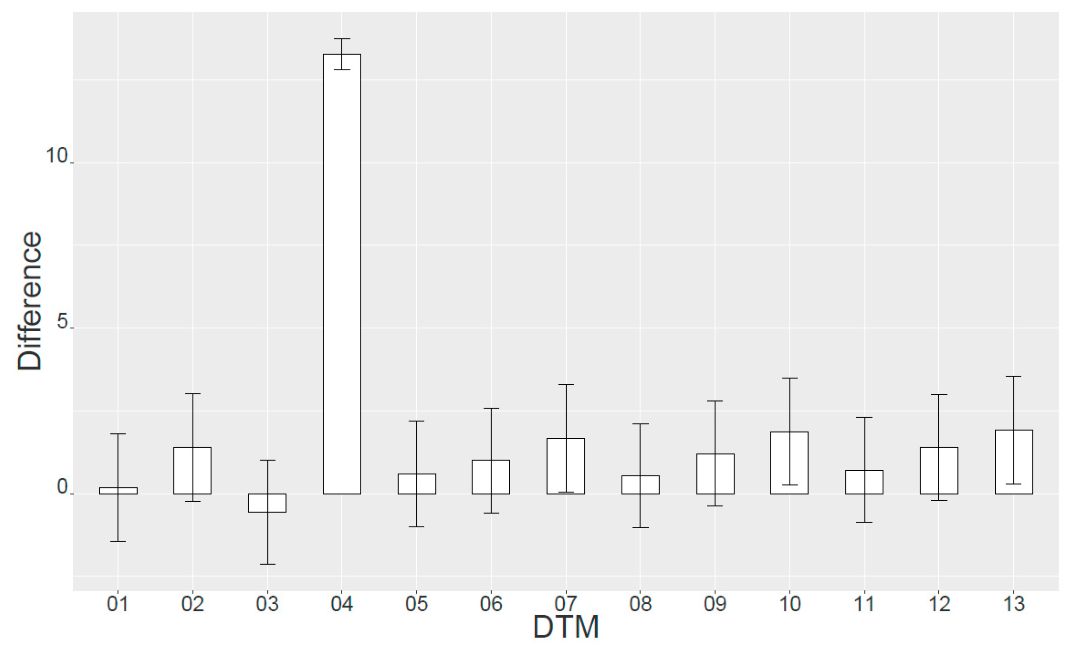
3.1. Comparison of the DTM Generation Methods

The initial results showed that there were statistically significant differences in height deviations from the GPS readings between the different DTMs (p < 0.001). However, when the values from SRTM (DTM 04) were excluded, the results indicated that there were no significant differences in height deviations from GPS readings (p = 0.997) amongst the remaining DTMs. Figure 4 displays the distribution of mean height differences of plot center values for GPS and corresponding DTMs.

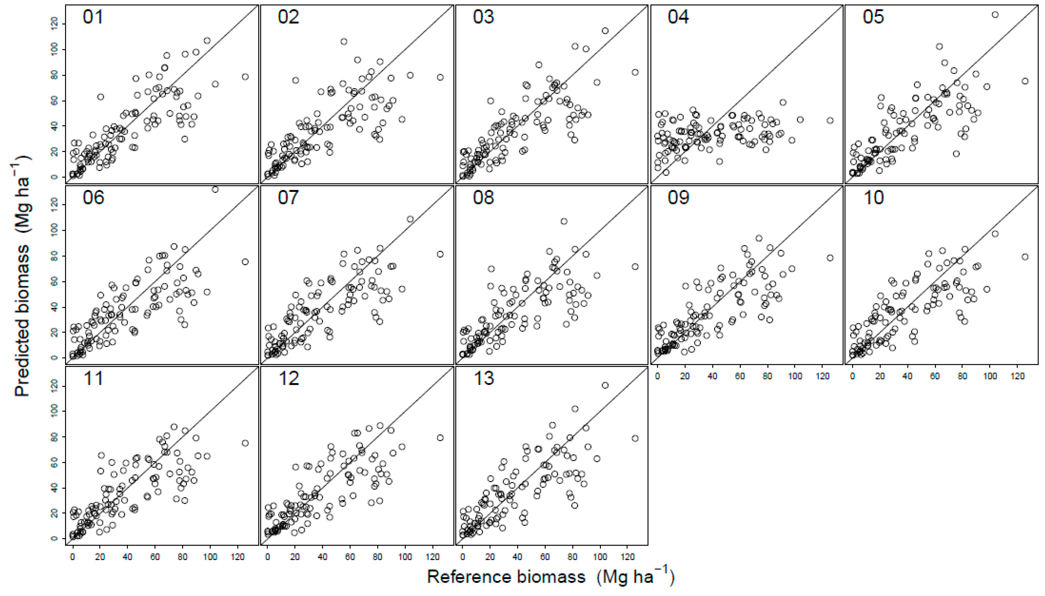
3.2. Regression Analysis

All the models produced appropriate model performance criteria, i.e., none of the models had MPE values that were significantly different from zero (p > 0.05) (

Table 4. Performance of models over different digital terrain models (DTMs) and ground classification approaches.

DTM 1	Independent Variables 2	r2	Predicted Biomass Mg·ha−1	RMSE		MPE		p-Value
				Mg·ha−1	%	Mg·ha−1	%
01	Hmax, D9, Ssd.blue	0.67	39.64	18.36	46.8	−0.41	−1.1	0.82
02	Hmax, D2, Ssd.green	0.58	39.26	21.44	55.0	−0.27	−0.7	0.90
03	Hmax, D5, Ssd.blue	0.65	39.21	18.73	48.0	−0.22	−0.6	0.91
04	S50.red	0.12	38.95	31.87	81.7	0.04	0.1	0.99
05	Hsd, D0, Ssd.blue	0.61	39.44	20.38	52.2	−0.45	−1.2	0.82
06	Hmax, S70.red, S90.green	0.61	39.15	19.76	50.7	−0.16	−0.4	0.93
07	Hmax, S70.red, S90.green	0.64	39.03	18.21	46.7	−0.03	−0.1	0.99
08	Hmax, D0, Ssd.blue	0.59	38.60	22.73	58.3	0.39	1.0	0.86
09	Hmax, D0, Scv.red	0.63	38.90	20.40	52.3	0.09	0.2	0.96
10	Hmax, S70.red, S90.green	0.62	39.02	19.54	50.1	−0.03	−0.1	0.99
11	Hmax, D0, Scv.green	0.62	39.03	20.36	52.2	−0.03	−0.1	0.99
12	Hmax, D0, Scv.red	0.62	38.90	19.68	50.5	0.09	0.2	0.96
13	Hmax, D0, S70.red, S90.green	0.63	39.69	20.19	51.8	−0.71	−1.8	0.72

¹ 01, DTM using supervised ground filtering based on visual classification; 02, DTM using supervised ground filtering based on logistic regression; 03, DTM using supervised ground filtering based on quantile regression; 04, DTM using unsupervised ground filtering based on shuttle radar topography mission (SRTM); 05–13, DTMs using unsupervised ground filtering based on a grid search approach for optimal parameter settings in Agisoft Photoscan Professional software (see Section 2.4. for details); ² S50.red, S70.red and S90.green: spectral variables for the 50%, 70% and 90 percentile for the red, red and green colour bands, respectively; D0, D2, D5 and D9: canopy densities corresponding to the proportions of points above fraction number 0, 2, 5 and 9, respectively; Hmax, Hsd, Scv.red, Scv.green, Ssd.green, Ssd.blue: maximum canopy height, canopy height standard deviation, coefficient of variation for the spectral variables with red and green colour bands respectively; standard deviation for the spectral variables with green and blue colour bands, r² = squared Pearson’s correlation coefficient, RMSE= Root mean square error, MPE = Mean prediction error.

). The models produced RMSE values in the range of 46.7%–81.7% of the mean biomass from ground reference biomass data (38.99 Mg·ha⁻¹). The r² values for all the models ranged from 0.12 to 0.67. Model 07, developed using unsupervised ground filtering based on a grid search approach, had the smallest RMSE% value amongst the models. Figure 5 displays the relationship between ground reference and predicted biomass for models 01–13. There is a general trend of under predictions for sample plots with higher biomass amongst all the models.

Amongst the developed models, approximately 20%, i.e., 13 out of 64 of the candidate independent variables, were selected. In total nine of the variables belonged to canopy height while the remaining four belonged to canopy density. Amongst the selected canopy height variables, Hmax, was the most frequently selected variable for the models.

In addition, all models (see Table 4) included spectral variables with the three color bands, red, green and blue. Amongst the models, the red color band was the most frequently selected.

4. Discussion

Successful implementation of the REDD+ initiative is dependent on the availability of reliable biomass estimating methods. Application of UAVs in monitoring forest ecosystems and in biomass estimation is gaining increased attention [28,63,64]. This study aimed at evaluating the application of 3D data generated from UAV acquired images in forest biomass estimation for the miombo woodlands. This could be of particular interest for Malawi since most of the forests in the country comprise of miombo woodlands scattered over the landscape as small- to medium sized reserves, a situation that suits the application of the UAV both when it comes to technical aspects and to costs associated with its execution.

Reliable biomass estimates from remotely sensed 3D data are heavily reliant on the availability of a good DTM. This study first tested different methods of generating DTMs. The comparisons of plot center height estimates from different DTMs showed that estimates from the DTM generated using SRTM data are unreliable as compared to the DTMs derived from the other methods (Figure 4). This indicates that when a DTM based on SRTM data is used for biomass estimation, the estimates can hardly be trusted. Despite the fact that there were no statistically significant differences amongst the DTMs developed from the different methods, i.e., excluding SRTM, the DTM model producing the smallest RMSE should always be applied when estimating biomass.

The biomass estimates based on five different approaches, with a total of 13 variants, showed that the DTM developed from unsupervised ground filtering based on a grid search approach (Model 07) performed slightly better than the other models (Table 4). This performance demonstrated that with some effort, it is possible to get a good combination of angle–distance parameter settings in the AgiSoft Photoscan software [49]. Furthermore, despite performing slightly poorer than Model 07, Model 01 developed from a DTM based on supervised ground filtering using visual classification, is equally good. However, the process of generating a DTM using supervised ground filtering based on visual classification is quite arduous. Therefore, since unsupervised ground filtering is easier to implement and performs equally (or even better) to visual classification, future studies should consider applying this approach. On the other hand, the relatively poor performance of the DTMs developed from unsupervised ground filtering based on shuttle radar topography mission (SRTM) could be attributed to the inherent random errors in heights associated with SRTM data [65,66,67].

The findings from our study demonstrated that data generated by the UAV system have potential of being successfully used in estimating forest biomass in dry tropical forests such as miombo woodlands. The fact that no MPE values were significantly different from zero (Table 4) is indicating that the models can be appropriately used in biomass estimation. Similar studies for other dry tropical forest sites are, however, recommended to validate the results from the current study because of the wide range of forest conditions seen in dry tropical forests such as miombo woodlands.

The observed RMSE% value for the best model from our study (46.7%) is similar to that reported in a study conducted in miombo woodlands of Tanzania (46.8%) by Mauya, et al. [36]. Direct comparison of these results should however be done with caution because ALS data were used in that study. In addition, there were differences in sample size, plot size and forest conditions for the respective studies.

In a study by Puliti, et al. [27] , where data acquired from UAV were applied in boreal forests, a RMSE% value of 14.95% was observed when estimating forest stand volume. The relatively low RMSE% as compared to the current study might be attributed to the differences in forest structures between miombo woodlands and boreal forests. It should also be noted that Puliti, et al. [27] utilized ALS data for DTM determination, which are superior in describing forest ground surface compared to optical sensors such as those applied in the current study [68]. It is worth noting that the observed RMSE% in Puliti, et al. [27] is comparable to that observed by Gobakken, et al. [69] conducted in similar forest conditions. However, Gobakken, et al. [69] used exclusively ALS data. This demonstrates the efficiency of UAV data in forest inventories.

During image acquisition, wind speeds up to 9.5 m·s⁻¹ were encountered. According to Dandois and Ellis [26], images captured when wind speeds are around or over 9.5 m·s⁻¹ generally make some trees sway as well as affect the UAV motion. This may result in incomplete image overlaps, which affect the quality of the generated point cloud and DTM for parts of a study area. We thus anticipated that this scenario would have some influence on the results. We also anticipated that the presence of shadow effects for some of the captured images could have had a profound effect on the results as is the case when photogrammetry is applied through traditional interpretation and automatic procedures, see e.g. Campbell and Wynne [70]. This is the case because automatic detection of reliable image features in areas of shadow is reportedly difficult due to large brightness ranges between shadows and sunlit areas. In addition, the properties and settings of the camera may result in insufficient image contrasts in areas of shadow [29]. Furthermore, we also anticipated that the leaf-on nature of the forest during data collection may have led to inaccurate interpolation of ground points due to uncertain point locations and low point density in areas of high canopy cover [16,29]. It is worth noting that despite the fact the data for the current study were collected under varying wind speed, light and terrain conditions, the results are similar with results from using ALS data [36].

The results from the current study demonstrate the ability of the UAV to capture reliable imagery under varying conditions in miombo woodlands. However, to fully comprehend the potential of utilizing UAV systems in miombo woodlands, future studies should aim at acquiring the images at times of a day when shadow effects are minimized, e.g., at noon as well as when wind speeds are low. However, it is often costly to wait for optimal weather conditions in remote sites due to associated logistical costs. Thus, the current study, together with the study by Puliti, et al. [27], are examples showing that it is still possible to obtain high accuracies under varying weather conditions. Acquiring images under leaf-off conditions might improve the ground classification, but might decrease the possibility to reconstruct trees in the point cloud and thus decrease biomass estimates. Acquiring imagery under both leaf-off and leaf-on conditions might provide the best results.

Furthermore, this study was conducted on a single site and thus represents a forest inventory scenario at a specific location. Similar studies should therefore be conducted in other reserves across the country in order to be able to generalize and provide guidance for application in cases such as NFIs. Future studies should also aim at evaluating the changes in precision and associated costs when estimating biomass for a forest reserve using 3D data from UAV imagery as auxiliary data, as compared to only using field data. For small to medium sized forest reserves, the methodology presented in this study seems directly applicable for obtaining high-resolution wall-to-wall 3D data, which are likely more robust in detecting biomass changes (e.g., degradation) than freely available satellite imagery such as Landsat [10]. However, as is the case with collecting field data, complete coverage of high-resolution wall-to-wall 3D data in large forest reserves will require substantial resources. It is therefore prudent to test the applicability of UAVs as a sampling tool in large forest reserves, as well as to compare with of other remotely sensed data, e.g., optical satellite imagery.

The importance of spectral information is highlighted by the selection of variables incorporating the red, green and blue color bands in all the generated models. According to Wallace, et al. [29], spectral components of UAV point clouds tend to present additional useful information for estimating other non- structural properties of the canopy. Similar results were also observed by [71] using satellite imagery data based on photogrammetric principles.

During the study a fixed plot size was used. However, the size of the field plots has been identified as one of the sources of model uncertainty in remote sensing based biomass estimation [36,72,73,74]. Future studies should therefore aim at examining the effects of field plot size, and even number of plots, on biomass estimates. Furthermore, during the study the images were acquired at a constant flight height of approximately 325 m above the ground. Future studies utilizing UAVs in Malawi could also aim at testing the effect of flight height on biomass estimates. Such a study would be possible because the directorate of civil aviation in Malawi does not currently impose any restrictions on flight height unlike in other countries where UAV flight heights are restricted by law [17,27,29,75].

5. Conclusions

The remotely sensed data captured using a SenseFly eBee fixed-wing UAV system was tested for biomass estimation on a small- to medium-sized potential REDD+ project site in miombo woodlands of Malawi. Except for the DTM based on SRTM, the differences between the tested DTMs were minor both when comparing to the heights derived from GPS recordings and to the final biomass estimates. Amongst the generated DTMs, the one developed using unsupervised ground filtering based on a grid search approach, had the smallest RMSE value of the biomass estimates. This indicates that DTMs developed through this method can produce reliable results in miombo woodlands. The observed prediction errors of the biomass estimates are similar to those from previous studies using ALS data in miombo woodlands. This is indicating the large potential of data derived from UAV imagery in estimation of biomass in miombo woodlands. However, for potential applications of UAV in forest inventories, either in full coverage or as a sampling tool, the biomass estimates and costs must be compared to alternative methods, such as pure field based inventories or in combination with auxiliary data from other remote sensing sources. Additional studies are also recommended to validate the results under other forest conditions using different flight settings, plot sizes and sample sizes.

References

1. Gibbs, H.K.; Brown, S.; Niles, J.O.; Foley, J.A. Monitoring and estimating tropical forest carbon stocks: Making REDD a reality. Environ. Res. Lett. 2007, 2, 045023. [Google Scholar] [CrossRef]
2. Government of Malawi. Government of Malawi REDD+ Action Plan 2014–2019; Department of Forestry, Ministry of Environment and Climate Change Management: Lilongwe, Malawi, 2015.
3. Tomppo, E.; Malimbwi, R.; Katila, M.; Mäkisara, K.; Henttonen, H.M.; Chamuya, N.; Zahabu, E.; Otieno, J. A sampling design for a large area forest inventory: Case Tanzania. Can. J. For. Res. 2014, 44, 931–948. [Google Scholar] [CrossRef]
4. Government of Malawi. Forest Resource Mapping Project under the Japanese Grant for the Forest Preservation Programme to the Republic of Malawi; Department of Forestry, Ministry of Environment and Climate Change Management: Lilongwe, Malawi, 2012.
5. Chidumayo, E.N. Miombo Ecology and Management: An Introduction; IT Publications in Association with the Stockholm Environment Institute: London, UK, 1997; p. 166. [Google Scholar]
6. Government of Malawi. Malawi State of Environment and Outlook Report; Ministry of Natural Resources, Energy and Environment: Lilongwe, Malawi, 2010.
7. Angelsen, A. Moving Ahead with REDD: Issues, Options and Implications; Center for International Forestry Research (CIFOR): Bogor, Indonesia, 2008. [Google Scholar]
8. DeFries, R.; Achard, F.; Brown, S.; Herold, M.; Murdiyarso, D.; Schlamadinger, B.; de Souza, C., Jr. Earth observations for estimating greenhouse gas emissions from deforestation in developing countries. Environ. Sci. Policy 2007, 10, 385–394. [Google Scholar] [CrossRef]
9. Sinha, S.; Jeganathan, C.; Sharma, L.; Nathawat, M. A review of radar remote sensing for biomass estimation. Int. J. Environ. Sci. Technol. 2015, 12, 1779–1792. [Google Scholar] [CrossRef]
10. Dube, T.; Mutanga, O. Evaluating the utility of the medium-spatial resolution landsat 8 multispectral sensor in quantifying aboveground biomass in uMgeni catchment, South Africa. ISPRS J. Photogramm. Remote Sens. 2015, 101, 36–46. [Google Scholar] [CrossRef]
11. McRoberts, R.E.; Næsset, E.; Gobakken, T.; Bollandsås, O.M. Indirect and direct estimation of forest biomass change using forest inventory and airborne laser scanning data. Remote Sens. Environ. 2015, 164, 36–42. [Google Scholar] [CrossRef]
12. Masek, J.G.; Hayes, D.J.; Joseph, H.M.; Healey, S.P.; Turner, D.P. The role of remote sensing in process-scaling studies of managed forest ecosystems. For. Ecol. Manag. 2015, 355, 109–123. [Google Scholar] [CrossRef]
13. Barrett, F.; McRoberts, R.E.; Tomppo, E.; Cienciala, E.; Waser, L.T. A questionnaire-based review of the operational use of remotely sensed data by national forest inventories. Remote Sens. Environ. 2016, 174, 279–289. [Google Scholar] [CrossRef]
14. Næsset, E.; Gobakken, T.; Bollandsås, O.M.; Gregoire, T.G.; Nelson, R.; Ståhl, G. Comparison of precision of biomass estimates in regional field sample surveys and airborne lidar-assisted surveys in Hedmark county, Norway. Remote Sens. Environ. 2013, 130, 108–120. [Google Scholar] [CrossRef]
15. Lu, D.; Chen, Q.; Wang, G.; Liu, L.; Li, G.; Moran, E. A survey of remote sensing-based aboveground biomass estimation methods in forest ecosystems. Int. J. Digit. Earth 2014, 1–43. [Google Scholar] [CrossRef]
16. Kumar, L.; Sinha, P.; Taylor, S.; Alqurashi, A.F. Review of the use of remote sensing for biomass estimation to support renewable energy generation. J. Appl. Remote Sens. 2015, 9, 29. [Google Scholar] [CrossRef]
17. Dandois, J.; Olano, M.; Ellis, E. Optimal altitude, overlap, and weather conditions for computer vision UAV estimates of forest structure. Remote Sens. 2015, 7, 13895–13920. [Google Scholar] [CrossRef]
18. Næsset, E.; Gobakken, T. Estimation of above- and below-ground biomass across regions of the boreal forest zone using airborne laser. Remote Sens. Environ. 2008, 112, 3079–3090. [Google Scholar] [CrossRef]
19. Skowronski, N.S.; Clark, K.L.; Gallagher, M.; Birdsey, R.A.; Hom, J.L. Airborne laser scanner-assisted estimation of aboveground biomass change in a temperate oak-pine forest. Remote Sens. Environ. 2014, 151, 166–174. [Google Scholar] [CrossRef]
20. Patenaude, G.; Hill, R.A.; Milne, R.; Gaveau, D.L.A.; Briggs, B.B.J.; Dawson, T.P. Quantifying forest above ground carbon content using lidar remote sensing. Remote Sens. Environ. 2004, 93, 368–380. [Google Scholar] [CrossRef]
21. Gonzalez, P.; Asner, G.P.; Battles, J.J.; Lefsky, M.A.; Waring, K.M.; Palace, M. Forest carbon densities and uncertainties from lidar, quickbird, and field measurements in California. Remote Sens. Environ. 2010, 114, 1561–1575. [Google Scholar] [CrossRef]
22. Drake, J.B.; Dubayah, R.O.; Clark, D.B.; Knox, R.G.; Blair, J.B.; Hofton, M.A.; Chazdon, R.L.; Weishampel, J.F.; Prince, S. Estimation of tropical forest structural characteristics using large-footprint lidar. Remote Sens. Environ. 2002, 79, 305–319. [Google Scholar] [CrossRef]
23. Mauya, E.; Hansen, E.; Gobakken, T.; Bollandsas, O.; Malimbwi, R.; Naesset, E. Effects of field plot size on prediction accuracy of aboveground biomass in airborne laser scanning-assisted inventories in tropical rain forests of Tanzania. Carbon Balance Manag. 2015, 10, 1–14. [Google Scholar] [CrossRef] [PubMed] [Green Version]
24. Vauhkonen, J.; Maltamo, M.; McRoberts, R.E.; Næsset, E. Introduction to forestry applications of airborne laser scanning. In Forestry Applications of Airborne Laser Scanning-Concepts and Case Studies; Maltamo, M., Næsset, E., Vauhkonen, J., Eds.; Springer: Dordrecht, The Netherlands, 2014; pp. 1–6. [Google Scholar]
25. Whitehead, K.; Hugenholtz, C.H. Remote sensing of the environment with small unmanned aircraft systems (UASs), part 1: A review of progress and challenges. J. Unmanned Veh. Syst. 2014, 2, 69–85. [Google Scholar] [CrossRef]
26. Dandois, J.P.; Ellis, E.C. High spatial resolution three-dimensional mapping of vegetation spectral dynamics using computer vision. Remote Sens. Environ. 2013, 136, 259–276. [Google Scholar] [CrossRef]
27. Puliti, S.; Ørka, H.; Gobakken, T.; Næsset, E. Inventory of small forest areas using an unmanned aerial system. Remote Sens. 2015, 7, 9632–9654. [Google Scholar] [CrossRef] [Green Version]
28. Tang, L.; Shao, G. Drone remote sensing for forestry research and practices. J. For. Res. 2015, 26, 791–797. [Google Scholar] [CrossRef]
29. Wallace, L.; Lucieer, A.; Malenovský, Z.; Turner, D.; Vopěnka, P. Assessment of forest structure using two UAV techniques: A comparison of airborne laser scanning and structure from motion (SfM) point clouds. Forests 2016, 7, 62. [Google Scholar] [CrossRef]
30. Siebert, S.; Teizer, J. Mobile 3D mapping for surveying earthwork projects using an unmanned aerial vehicle (UAV) system. Autom. Constr. 2014, 41, 1–14. [Google Scholar] [CrossRef]
31. Getzin, S.; Wiegand, K.; Schöning, I. Assessing biodiversity in forests using very high-resolution images and unmanned aerial vehicles. Methods Ecol. Evol. 2012, 3, 397–404. [Google Scholar] [CrossRef]
32. Chidumayo, E.N. Forest degradation and recovery in a miombo woodland landscape in Zambia: 22 years of observations on permanent sample plots. For. Ecol. Manag. 2013, 291, 154–161. [Google Scholar] [CrossRef]
33. Chidumayo, E.N.; Gumbo, D.J. The Dry Forests and Woodlands of Africa: Managing for Products and Services; Earthscan: London, UK, 2010. [Google Scholar]
34. Næsset, E.; Økland, T. Estimating tree height and tree crown properties using airborne scanning laser in a boreal nature reserve. Remote Sens. Environ. 2002, 79, 105–115. [Google Scholar] [CrossRef]
35. Ravindranath, N.H.; Ostwald, M. Carbon Inventory Methods—Handbook for Greenhouse Gas Inventory, Carbon Mitigation and Roundwood Production Projects; Springer: Heidelberg, Germany, 2008; Volume 29. [Google Scholar]
36. Mauya, E.; Ene, L.; Bollandsås, O.; Gobakken, T.; Næsset, E.; Malimbwi, R.; Zahabu, E. Modelling aboveground forest biomass using airborne laser scanner data in the miombo woodlands of Tanzania. Carbon Balance Manag. 2015, 10, 28. [Google Scholar] [CrossRef] [PubMed] [Green Version]
37. Gregoire, T.G.; Næsset, E.; McRoberts, R.E.; Ståhl, G.; Andersen, H.-E.; Gobakken, T.; Ene, L.; Nelson, R. Statistical rigor in lidar-assisted estimation of aboveground forest biomass. Remote Sens. Environ. 2016, 173, 98–108. [Google Scholar] [CrossRef]
38. Yang, J.; Prince, S.D. Remote sensing of savanna vegetation changes in eastern Zambia 1972–1989. Int. J. Remote Sens. 2000, 21, 301–322. [Google Scholar] [CrossRef]
39. Fuller, D.O.; Prince, S.D.; Astle, W.L. The influence of canopy strata on remotely sensed observations of savanna-woodlands. Int. J. Remote Sens. 1997, 18, 2985–3009. [Google Scholar] [CrossRef]
40. Maguya, A.; Junttila, V.; Kauranne, T. Algorithm for extracting digital terrain models under forest canopy from airborne lidar data. Remote Sens. 2014, 6, 6524–6548. [Google Scholar] [CrossRef]
41. Niethammer, U.; James, M.R.; Rothmund, S.; Travelletti, J.; Joswig, M. UAV-based remote sensing of the super-sauze landslide: Evaluation and results. Eng. Geol. 2012, 128, 2–11. [Google Scholar] [CrossRef]
42. Soininen, A. Terrascan User’s Guide; Terrasolid: Helsinki, Finland, 2004. [Google Scholar]
43. McGaughey, R. FUSION/LDV: Software for LIDAR Data Analysis and Visualization; version 3.50; United States Department of Agriculture (USDA), Forest Service, Pacific Northwest Research Station: Portland, OR, USA, 2015.
44. Hardcastle, P.D. A Preliminary Silvicultural Classification of Malawi; Forestry Research Institute of Malawi: Zomba, Malawi, 1978. [Google Scholar]
45. Kouba, J. A Guide to Using International Gnss Service (IGS) Products; Geodetic Survey Division, Natural Resources Canada: Ottawa, ON, Canada, 2015. [Google Scholar]
46. Takasu, T. RTKLIB: Open Source Program Package for RTK-GPS; Free and Open Source Software for Geospatial Sydney; Open Source Geospatial Foundation (OSGeo): Sydney, Australia, 2009. [Google Scholar]
47. Kachamba, D.J.; Eid, T.; Gobakken, T. Above- and belowground biomass models for trees in the miombo woodlands of Malawi. Forests 2016, 7, 38. [Google Scholar] [CrossRef]
48. Sensefly. Ebee Sensefly: Extended User Manual; Sensefly, Ltd.: Cheseaux-Lausanne, Switzerland, 2015. [Google Scholar]
49. AgiSoft. Agisoft Photoscan User Manual: Professional Edition, version 1.1; AgiSoft LLC: St. Petersburg, Russia, 2015. [Google Scholar]
50. Stal, C.; Briese, C.; De Maeyer, P.; Dorninger, P.; Nuttens, T.; Pfeifer, N.; De Wulf, A. Classification of airborne laser scanning point clouds based on binomial logistic regression analysis. Int. J. Remote Sens. 2014, 35, 3219–3236. [Google Scholar] [CrossRef] [Green Version]
51. Cade, B.S.; Noon, B.R. A gentle introduction to quantile regression for ecologists. Front. Ecol. Environ. 2003, 1, 412–420. [Google Scholar] [CrossRef]
52. Fahrmeir, L.; Kneib, T.; Lang, S.; Marx, B. Regression; Springer: Berlin/Heidelberg, Germany, 2013; p. 698. [Google Scholar]
53. Van Zyl, J.J. The shuttle radar topography mission (srtm): A breakthrough in remote sensing of topography. Acta Astronaut. 2001, 48, 559–565. [Google Scholar] [CrossRef]
54. Axelsson, P. Processing of laser scanner data-algorithms and applications. ISPRS J. Photogramm. Remote Sens. 1999, 54, 138–147. [Google Scholar] [CrossRef]
55. Næsset, E. Practical large-scale forest stand inventory using a small-footprint airborne scanning laser. Scand. J. For. Res. 2004, 19, 164–179. [Google Scholar] [CrossRef]
56. Næsset, E.; Bollandsås, O.M.; Gobakken, T. Comparing regression methods in estimation of biophysical properties of forest stands from two different inventories using laser scanner data. Remote Sens. Environ. 2005, 94, 541–553. [Google Scholar] [CrossRef]
57. White, J.; Wulder, M.; Varhola, A.; Vastaranta, M.; Coops, N.; Cook, B.; Pitt, D.; Woods, M. A Best Practices Guide for Generating Forest Inventory Attributes from Airborne Laser Scanning Data Using an Area-Based Approach (Version 2.0); Natural Resources Canada: Ottawa, ON, Canada, 2013; p. 50. [Google Scholar]
58. Lumley, T. Leaps: Regression subset selection. In R Package, version 2.9; R Core Team: Vienna, Austria, 2009. [Google Scholar]
59. R Core Team. R: A Language and Environment for Statistical Computing; R Foundation for Statistical Computing: Vienna, Austria, 2016. [Google Scholar]
60. Meng, J.; Li, S.; Wang, W.; Liu, Q.; Xie, S.; Ma, W. Mapping forest health using spectral and textural information extracted from spot-5 satellite images. Remote Sens. 2016, 8, 719. [Google Scholar] [CrossRef]
61. Snowdon, P. A ratio estimator for bias correction in logarithmic regressions. Can. J. For. Res. 1991, 21, 720–724. [Google Scholar] [CrossRef]
62. James, G.; Witten, D.; Hastie, T.; Tibshirani, R. An Introduction to Statistical Learning with Application in R; Springer: New York, NY, USA, 2013; Volume 103. [Google Scholar]
63. Zhang, J.; Hu, J.; Lian, J.; Fan, Z.; Ouyang, X.; Ye, W. Seeing the forest from drones: Testing the potential of lightweight drones as a tool for long-term forest monitoring. Biol. Conserv. 2016, 198, 60–69. [Google Scholar] [CrossRef]
64. Chianucci, F.; Disperati, L.; Guzzi, D.; Bianchini, D.; Nardino, V.; Lastri, C.; Rindinella, A.; Corona, P. Estimation of canopy attributes in beech forests using true colour digital images from a small fixed-wing UAV. Int. J. Appl. Earth Obs. Geoinf. 2016, 47, 60–68. [Google Scholar] [CrossRef] [Green Version]
65. Rodríguez, E.; Morris, C.; Belz, J. A global assessment of the srtm performance. Photogramm. Eng. Remote Sens. 2006, 72, 249–260. [Google Scholar] [CrossRef]
66. Karwel, A.; Ewiak, I. Silk road for information from imagery. In Estimation of the Accuracy of the SRTM Terrain Model on the Area of Poland; Chen, J., Jiang, J., Genderen, J.V., Eds.; International Society for Photogrammetry and Remote Sensing: Beijing, China, 2008; pp. 169–172. [Google Scholar]
67. Hofton, M.; Dubayah, R.; Blair, J.; Rabine, D. Validation of srtm elevations over vegetated and non-vegetated terrain using medium footprint lidar. Photogramm. Eng. Remote Sens. 2006, 72, 279–285. [Google Scholar] [CrossRef]
68. Baltsavias, E.P. A comparison between photogrammetry and laser scanning. ISPRS J. Photogramm. Remote Sens. 1999, 54, 83–94. [Google Scholar] [CrossRef]
69. Gobakken, T.; Bollandsås, O.M.; Næsset, E. Comparing biophysical forest characteristics estimated from photogrammetric matching of aerial images and airborne laser scanning data. Scand. J. For. Res. 2015, 30, 73–86. [Google Scholar] [CrossRef]
70. Campbell, J.B.; Wynne, R.H. Introduction to Remote Sensing; Guilford Press: New York, NY, USA, 2011. [Google Scholar]
71. Immitzer, M.; Stepper, C.; Böck, S.; Straub, C.; Atzberger, C. Use of worldview-2 stereo imagery and national forest inventory data for wall-to-wall mapping of growing stock. For. Ecol. Manag. 2016, 359, 232–246. [Google Scholar] [CrossRef]
72. Frazer, G.; Magnussen, S.; Wulder, M.; Niemann, K. Simulated impact of sample plot size and co-registration error on the accuracy and uncertainty of lidar-derived estimates of forest stand biomass. Remote Sens. Environ. 2011, 115, 636–649. [Google Scholar] [CrossRef]
73. Keller, M.; Palace, M.; Hurtt, G. Biomass estimation in the tapajos national forest, brazil: Examination of sampling and allometric uncertainties. For. Ecol. Manag. 2001, 154, 371–382. [Google Scholar] [CrossRef]
74. Hansen, E.; Gobakken, T.; Bollandsas, O.; Zahabu, E.; Naesset, E. Modeling aboveground biomass in dense tropical submontane rainforest using airborne laser scanner data. Remote Sens. 2015, 7, 788–807. [Google Scholar] [CrossRef] [Green Version]
75. Zahawi, R.A.; Dandois, J.P.; Holl, K.D.; Nadwodny, D.; Reid, J.L.; Ellis, E.C. Using lightweight unmanned aerial vehicles to monitor tropical forest recovery. Biol. Conserv. 2015, 186, 287–295. [Google Scholar] [CrossRef]
Figure 1. Miombo woodlands in Muyobe forest reserve, Malawi (Photos: Hans Ole Ørka).
Remotesensing 08 00968 g001
Figure 2. Map of Malawi showing the location of the study site.
Remotesensing 08 00968 g002
Figure 3. Schematic diagram for the different DTM generation approaches.
Remotesensing 08 00968 g003
Figure 4. Mean height differences (m) between measured GPS (reference values) and predicted heights for the different DTM generation methods with standard errors: 01, DTM using supervised ground filtering based on visual classification; 02, DTM using supervised ground filtering based on logistic regression; 03, DTM using supervised ground filtering based on quantile regression; 04, DTM using unsupervised ground filtering based on shuttle radar topography mission (SRTM); and 05–13, DTMs using unsupervised ground filtering based on a grid search approach for optimal parameter settings in Agisoft Photoscan Professional software (See Section 2.4. for details).
Remotesensing 08 00968 g004
Figure 5. Ground reference versus predicted biomass for different DTMs: 01, DTM using supervised ground filtering based on visual classification; 02, DTM using supervised ground filtering based on logistic regression; 03, DTM using supervised ground filtering based on quantile regression; 04, DTM using unsupervised ground filtering based on shuttle radar topography mission (SRTM); and 05–13, DTMs using unsupervised ground filtering based on a grid search approach for optimal parameter settings in Agisoft Photoscan Professional software (see Section 2.4. for details).
Remotesensing 08 00968 g005