Two Component Decomposition of Dual Polarimetric HH/VV SAR Data: Case Study for the Tundra Environment of the Mackenzie Delta Region, Canada

Abstract

This study investigates a two component decomposition technique for HH/VV-polarized PolSAR (Polarimetric Synthetic Aperture Radar) data. The approach is a straight forward adaption of the Yamaguchi decomposition and decomposes the data into two scattering contributions: surface and double bounce under the assumption of a negligible vegetation scattering component in Tundra environments. The dependencies between the features of this two and the classical three component Yamaguchi decomposition were investigated for Radarsat-2 (quad) and TerraSAR-X (HH/VV) data for the Mackenzie Delta Region, Canada. In situ data on land cover were used to derive the scattering characteristics and to analyze the correlation among the PolSAR features. The double bounce and surface scattering features of the two and three component scattering model (derived from pseudo-HH/VV- and quad-polarized data) showed similar scattering characteristics and positively correlated-R² values of 0.60 (double bounce) and 0.88 (surface scattering) were observed. The presence of volume scattering led to differences between the features and these were minimized for land cover classes of low vegetation height that showed little volume scattering contribution. In terms of separability, the quad-polarized Radarsat-2 data offered the best separation of the examined tundra land cover types and will be best suited for the classification. This is anticipated as it represents the largest feature space of all tested ones. However; the classes “wetland” and “bare ground” showed clear positions in the feature spaces of the C- and X-Band HH/VV-polarized data and an accurate classification of these land cover types is promising. Among the possible dual-polarization modes of Radarsat-2 the HH/VV was found to be the favorable mode for the characterization of the aforementioned tundra land cover classes due to the coherent acquisition and the preserved co-pol. phase. Contrary, HH/HV-polarized and VV/VH-polarized data were found to be best suited for the characterization of mixed and shrub dominated tundra.

1. Introduction

The decomposition of Polarimetric Synthetic Aperture Radar (PolSAR) data is an important analysis step to characterize different types of backscatter and to derive higher level (beyond level 2.0) products for earth observation. During the last decades much attention was paid to the decomposition of quad-polarized Synthetic Aperture Radar (SAR) data [1,2,3,4,5] and on the utilization of compact polarimetric systems (exemplarily: [6,7]). However, there are fewer concepts on the decomposition of dual-polarized data [8,9,10]. This type of PolSAR data advances higher spatial resolution and larger area coverage compared to the quad-polarized mode. Moreover, it offers higher signal-to-noise ratio (SNR) compared to the quad-pol data. Exemplarily, Cloude [8] showed the application of the mathematical, eigen-based Entropy/Alpha decomposition for dual polarimetric data. Since most of today’s systems—like Radarsat-2 (R-2), Sentinel-1 or ALOS-2—provide only HH/HV- or VV/VH-polarized data operationally, most attention was paid on the analyses of these types of dual-polarized data. With TerraSAR-X (TSX), TanDEM-X (TDX), and COSMO-Skymed an increasing number of high resolution SAR systems is capable of acquiring HH/VV-polarized data phase-coherently. Hence, co-polarimetric phase as well as amplitude information of the complex SAR measurement is available for the analysis. Therefore, this kind of data also allows investigating the polarimetric phase-relation between the HH and VV channels. This information is known to be an important discriminator for the characterization of surface and double bounce scattering, respectively of odd and even bounce [1,5].

Studies that highlight the benefit and applicability of HH/VV-polarized data for land cover characterization and classification are briefly named in the following. A decomposition scheme for HH/VV-polarized data was presented by Jagdhuber et al. [11,12] in the context of soil moisture estimation under agricultural vegetation. The approach utilizes a model-based volume component removal including the generation of synthetic cross-polarization (via the coherence of the complex HH and VV signals) and the dual-polarimetric eigen-based decomposition to retrieve the surface soil signal. The phase-relation of HH and VV was also investigated by Lopez-Sanchez et al. [13], who applied an eigen-based decomposition to TerraSAR-X HH/VV-polarized data. The findings indicated the usefulness of these dual-polarized data for the characterization of the type of scattering that was examined in the context of time series analyses for the retrieval of rice phenology (surface or double bounce scattering). Differences between the eigen-based decomposition features of HH/VV-polarized compared to quad-polarized data were investigated by [14]. Mitsunobu et al. [14] and showed a strong relation of the scattering angles. Voormansik et al. [15] investigated the potential of HH/VV dual-polarized TSX-data for studying grassland and to work towards the assessment of cutting practices on meadows. Heine et al. [16] used co-polarized TSX-data in time series for the analysis of phenological changes of wetland vegetation and showed that parameters sensitive to the double bounce revealed meaningful seasonal changes for reed belts. Further, Schmitt et al. [17] examined the Entropy/Alpha and Freeman-Durden decomposition models, as well as, the elements of the normalized Kennaugh Matrix of quad-polarized data for the characterization and classification of wetland vegetation. The findings indicated that HH and VV information were crucial for the characterization and pointed to the high effectiveness and applicability of HH/VV-polarized data that maintain higher spatial resolution and coverage compared to quad-polarized data.

The application of SAR and PolSAR data has special relevance for Arctic environments since the application of multispectral, respectively optical imaging is limited in this region, due to the short length of the growing season and the rapid phenological seasonal response of the tundra vegetation. In this context the frequent cloud cover of the high latitudes hinders the acquisition of optical data suited for time series analysis. A further challenge is the solar geometry: multispectral imaging is restricted to the summer months when the illumination conditions cause a large range of zenith and azimuth angles that complicate the image analysis [18]. Even though active radar remote sensing can overcome most of these problems, there are comparably few studies that incorporate SAR/PolSAR data for land surface characterization of Arctic environment; exemplary [19,20,21,22,23,24,25,26,27,28]. Possible reasons for this “lack of usage” are the difficult image interpretation, the unknown relation between SAR/PolSAR scattering and Arctic land surface properties and the restricted access to the data. At least the last point is becoming obsolete for C-Band SAR data with the operation of the Sentinel-1 satellites.

This study presents analyses of HH/VV-polarized data for the tundra environment of the Mackenzie Delta Region, Canada using C-Band R-2 and X-Band TSX/TDX data. Special emphasis is given on a two component, polarimetric decomposition of the dual-polarized data using a model that is a straight forward adaption of the model purposed for quad-polarized data by Yamaguchi et al. [29]. To our best knowledge such a straight forward adaptation of the Yamaguchi decomposition was never tested for HH/VV SAR data, beside our preliminary experiments [26,30]. The aim is to enhance the interpretability of the HH/VV SAR signal via the characterization of scattering mechanisms and to express the dual-polarized information in terms of scattering power components—similar to the Freeman-Durden and Yamaguchi decomposition models that are frequently applied to quad-polarized data. Further, its scope is to identify the benefit of polarimetry and to increase the understanding of scattering and backscatter formation in tundra environment and to propose techniques that enable better and more accurate classifications of the Arctic land surface.

2. Materials and Methods

2.1. Two Component Decomposition of HH/VV Data

Working with coherent HH/VV-polarized data, information of both channels HH and VV may be expressed by the coherency matrix $\mathrm{T}$. The matrix is derived by multiplying the two component target Pauli vector ${\mathrm{k}}_{\mathsf{\tau }}$ (Equation (1)) with its conjugate transpose ${\mathrm{k}}_{\mathsf{\tau }}^{+}$ (Equation (2)). $\mathrm{T}$ is a Hermitian matrix with two by two elements (Equation (3)) and represents the upper square sub-matrix of the full 3 × 3 coherency matrix of a quad-polarized measurement. The matrix elements are linear combinations of the complex HH- and VV-channels, based on the Pauli spin matrices [2] (Equation (4)). $\mathrm{T}$ can be used to exploit the phase difference of HH and VV channels: This relation is known to be a crucial discriminator for the characterization of the type of backscattering [1,31]; more precisely the discrimination between odd- and even-bounce scattering.

$${\mathrm{k}}_{\mathsf{\tau }}=\frac{1}{\surd 2}\left(\begin{array}{c}{\mathrm{S}}_{\mathrm{HH}}+{\mathrm{S}}_{\mathrm{VV}}\\ {\mathrm{S}}_{\mathrm{HH}}-{\mathrm{S}}_{\mathrm{VV}}\end{array}\right)$$

(1)

$$\mathrm{T}={\mathrm{k}}_{\mathsf{\tau }}{\mathrm{k}}_{\mathsf{\tau }}^{+}=\left[\begin{array}{cc}{\mathrm{T}}_{11}& {\mathrm{T}}_{12}\\ {\mathrm{T}}_{21}& {\mathrm{T}}_{22}\end{array}\right]$$

(2)

$$\mathrm{T}=\frac{1}{2}\langle \left[\begin{array}{cc}\left({\mathrm{S}}_{\mathrm{HH}}+{\mathrm{S}}_{\mathrm{VV}}\right){\left({\mathrm{S}}_{\mathrm{HH}}+{\mathrm{S}}_{\mathrm{VV}}\right)}^{\ast }& \left({\mathrm{S}}_{\mathrm{HH}}+{\mathrm{S}}_{\mathrm{VV}}\right){\left({\mathrm{S}}_{\mathrm{HH}}-{\mathrm{S}}_{\mathrm{VV}}\right)}^{\ast }\\ \left({\mathrm{S}}_{\mathrm{HH}}-{\mathrm{S}}_{\mathrm{VV}}\right){\left({\mathrm{S}}_{\mathrm{HH}}+{\mathrm{S}}_{\mathrm{VV}}\right)}^{\ast }& \left({\mathrm{S}}_{\mathrm{HH}}-{\mathrm{S}}_{\mathrm{VV}}\right){\left({\mathrm{S}}_{\mathrm{HH}}-{\mathrm{S}}_{\mathrm{VV}}\right)}^{\ast }\end{array}\right]\rangle$$

(3)

In the formulas ${}^{\ast }$ denotes the complex conjugate, ${}^{+}$ the conjugate transpose, and $\langle \rangle$ refers to the spatial averaging. Yamaguchi et al. [29] introduced a modified four component scattering model for quad-polarized data based on the decomposition concept of Freeman and Durden [32]. The approach of Yamaguchi et al. [29] is decomposing the full 3 × 3 coherency matrix into four signal components of surface scattering, double bounce, volume, and helix scattering (so-called power components). The method utilizes the model for the Bragg scattering via reflection coefficients that rely on the co-polarized information alone. The coefficients of $\mathsf{\alpha }$ and $\mathsf{\beta }$ are defined as stated in the original approach of Yamaguchi et al. [29] and display the orientation and characteristic of the scattered wave [5], thus these coefficients contain the “polarimetric information” and are called the “scattering mechanisms”. The decomposition model of Yamaguchi et al. [29] can be realized as a three component model, which is the more frequently applied approach. The model then decomposes the full 3 × 3 coherency matrix $\mathrm{T}$ into the features surface, double bounce, and volume scattering. A straight forward adaption of this approach for HH/VV-polarized SAR data is the decomposition of the span into the scattering power components of surface (${\mathrm{P}}_{\mathrm{s}}$) and double bounce (${\mathrm{P}}_{\mathrm{d}}$) scattering neglecting volume scattering: The estimation of these parameters is based on the co-polarized information alone. Such a two component decomposition model can be designed assuming no contribution of the cross-polarized channels on the respective co-polarized channels as shown in Equations (5) and (6).

$${\mathrm{P}}_{\mathrm{T}}={\mathrm{P}}_{\mathrm{s}}+{\mathrm{P}}_{\mathrm{d}}=\left[\begin{array}{cc}{\mathrm{T}}_{11}& {\mathrm{T}}_{12}\\ {\mathrm{T}}_{21}& {\mathrm{T}}_{22}\end{array}\right]={\mathrm{f}}_{\mathrm{s}}\left[\begin{array}{cc}1& {\mathsf{\beta }}^{\ast }\\ \mathsf{\beta }& {\left|\mathsf{\beta }\right|}^2\end{array}\right]+{\mathrm{f}}_{\mathrm{d}}\left[\begin{array}{cc}{\left|\mathsf{\alpha }\right|}^2& \mathsf{\alpha }\\ {\mathsf{\alpha }}^{\ast }& 1\end{array}\right]$$

(4)

The definition of the model leads to the three equations shown in Equations (5)–(7). The equation system has four unknowns ${\mathrm{f}}_{\mathrm{s}}$, ${\mathrm{f}}_{\mathrm{d}}$, $\mathsf{\alpha }$, and $\mathsf{\beta }$, and is therewith underdetermined. The unknowns ${\mathrm{f}}_{\mathrm{s}}$ and ${\mathrm{f}}_{\mathrm{d}}$ are the intensity components of the two scattering components to be determined [29]. The left hand side is given by the measured values of ${\mathrm{T}}_{11}$, ${\mathrm{T}}_{12}$, ${\mathrm{T}}_{21}$, and ${\mathrm{T}}_{22}$ of the HH/VV-polarized Coherency Matrix $\mathrm{T}$.

$${\mathrm{T}}_{11}=0.5\langle {\left|{\mathrm{S}}_{\mathrm{HH}}+{\mathrm{S}}_{\mathrm{VV}}\right|}^2\rangle ={\mathrm{f}}_{\mathrm{s}}+{\mathrm{f}}_{\mathrm{d}}{\left|\mathsf{\alpha }\right|}^2$$

(5)

$${\mathrm{T}}_{22}=0.5\langle {\left|{\mathrm{S}}_{\mathrm{HH}}-{\mathrm{S}}_{\mathrm{VV}}\right|}^2\rangle ={\mathrm{f}}_{\mathrm{d}}+{\mathrm{f}}_{\mathrm{s}}{\left|\mathsf{\beta }\right|}^2$$

(6)

$${\mathrm{T}}_{12}=0.5\langle \left({\mathrm{S}}_{\mathrm{HH}}+{\mathrm{S}}_{\mathrm{VV}}\right){\left({\mathrm{S}}_{\mathrm{HH}}-{\mathrm{S}}_{\mathrm{VV}}\right)}^{\ast }\rangle ={\mathrm{f}}_{\mathrm{d}}\mathsf{\alpha }+{\mathrm{f}}_{\mathrm{s}}{\mathsf{\beta }}^{\ast }$$

(7)

Two cases can be distinguished to simplify the equation system in order to be uniquely solvable; Case 1 with dominant surface scattering (${\mathrm{T}}_{11}>{\mathrm{T}}_{22}\mathrm{and}\mathsf{\alpha }=0$) and Case 2, with dominant double bounce scattering (${\mathrm{T}}_{22}>{\mathrm{T}}_{11}{\mathrm{and}\mathsf{\beta }}^{\ast }=0$), where the non-dominant scattering contribution is set to zero [5]. These definitions are identical to the original models of Yamaguchi and Freeman-Durden. The unknowns ${\mathrm{f}}_{\mathrm{s}}$, ${\mathrm{f}}_{\mathrm{d}}$, $\mathsf{\alpha }$ or $\mathsf{\beta }$ are then defined by Equations (8)–(10) for Case 1 and by Equations (11)–(13) for Case 2.

Case 1: ${\mathrm{T}}_{11}>{\mathrm{T}}_{22},\mathrm{with}\mathsf{\alpha }=0$:

$${\mathrm{f}}_{\mathrm{s}}={\mathrm{T}}_{11}$$

(8)

$${\mathrm{f}}_{\mathrm{d}}={\mathrm{T}}_{22}-\left(\frac{{\left|{\mathrm{T}}_{12}\right|}^2}{{\mathrm{T}}_{11}}\right)$$

(9)

$${\mathsf{\beta }}^{\ast }=\frac{{\mathrm{T}}_{12}}{{\mathrm{T}}_{11}}$$

(10)

Case 2: ${\mathrm{T}}_{22}>{\mathrm{T}}_{11},{\mathrm{with}\mathsf{\beta }}^{\ast }=0$:

$${\mathrm{f}}_{\mathrm{d}}={\mathrm{T}}_{22}$$

(11)

$${\mathrm{f}}_{\mathrm{s}}=T_{11}-\left(\frac{{\left|{\mathrm{T}}_{12}\right|}^2}{{\mathrm{T}}_{22}}\right)$$

(12)

$$\mathsf{\alpha }=\frac{{\mathrm{T}}_{12}}{{\mathrm{T}}_{22}}$$

(13)

The scattering power components ${\mathrm{P}}_{\mathrm{s}}$ and ${\mathrm{P}}_{\mathrm{d}}$ can be derived via Equations (14) and (15) consistently for both cases:

$${\mathrm{P}}_{\mathrm{s}}={\mathrm{f}}_{\mathrm{s}}(1+{\left|\mathsf{\beta }\right|}^2)$$

(14)

$${\mathrm{P}}_{\mathrm{d}}={\mathrm{f}}_{\mathrm{d}}(1+{\left|\mathsf{\alpha }\right|}^2)$$

(15)

The differences between the decomposition features of this two component model and of the three component model of [29] are the assumption of the absence of a significant volume scattering contribution and a volume-induced depolarization, respectively. This means the cross-polarized information will be ignored and is not measured for dual-polarimetric T. For real world applications one should take into account that a zero contribution of the cross-polarized channels—respectively an observation of ${\mathrm{T}}_{33}=0$ in terms of quad-polarized coherency matrix—is not a likely situation for radar observations of natural surfaces [1]. Furthermore, zero elements in the off-diagonal positions ${\mathrm{T}}_{13/31}$ and ${\mathrm{T}}_{23/32}$ of quad-polarized coherency matrices are only observable when no coherence between cross- and co-polarized channels is present [1] due to reflection symmetry for example. Nevertheless, this is a quite frequently applied symmetry assumption for natural media [5,29].

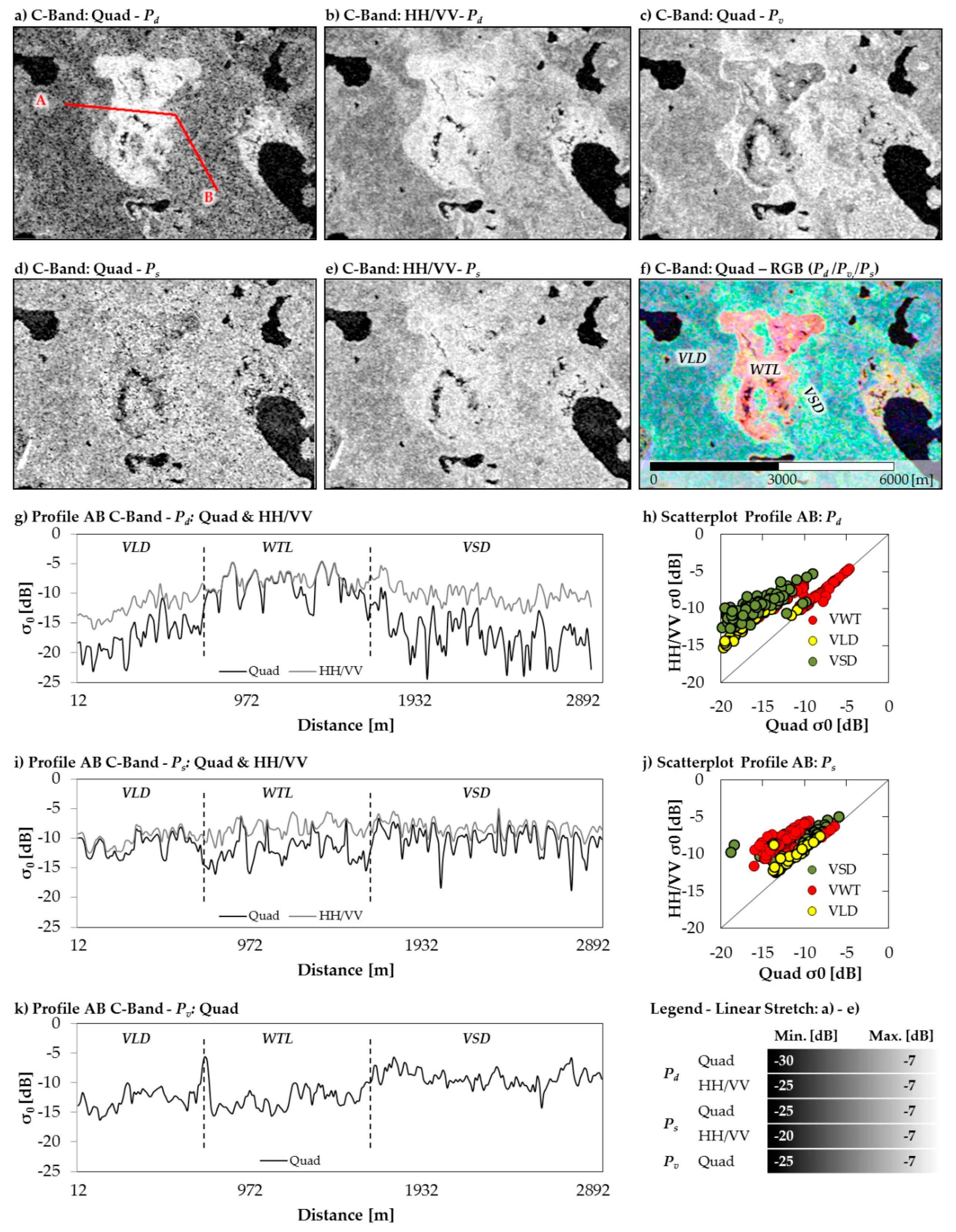
Accordingly, the correlations of ${\mathrm{P}}_{\mathrm{s}}$ and ${\mathrm{P}}_{\mathrm{d}}$ between the two and three component decomposition models is expected to be high for land cover types, e.g., bare or sparsely vegetated ground, that show no significant volume scattering with respect to the used wavelength and the spatial resolution. Contrary, the differences will be maximized for urban areas and for densely vegetated ground like forests: for such land cover types the contribution of volume scattering is usually high and not negligible at all. In comparison to the simple Pauli decomposition the discrimination between double-bounce (or even bounce in Pauli’s definition) and surface scattering (or odd bounce in the Pauli notation) is enhanced by introducing the polarimetric scattering mechanisms $\mathsf{\alpha }$ and $\mathsf{\beta }$ in Equations (14) and (15). The idea is to understand both, the intensity (${\mathrm{f}}_{\mathrm{s}}$, ${\mathrm{f}}_{\mathrm{d}}$) and the scattering mechanisms ($\mathsf{\alpha }$, $\mathsf{\beta }$) by using also the coherent nature of the data and not only the incoherent channel intensities (like for the Pauli decomposition of multi-looked images). Moreover, the Pauli decomposition would only distinguish between odd and even bounce scattering (multiple bounces) and not directly between surface and double-bounce scattering. So higher order scattering is actually not expected for tundra and just pure surface or dihedral scattering should be present, as the vegetation is low and comparably simple in structure. Thus, land cover discrimination and PolSAR signal interpretation is expected to be easier than using just the simple elements of the Coherency matrix.

2.2. PolSAR Database

We investigated quad-polarized R-2 and HH/VV-polarized TSX/TDX data of the Arctic Mackenzie Delta Region (Canada) in order to test the proposed decomposition approach and to examine the PolSAR signal in relation to the land coverage. This Arctic region exhibits a variety of land cover types on small scale and the transition between taiga and tundra ecosystems [33]. Figure 1 shows the location of the site and field photographs of frequent land cover types. The PolSAR data were acquired in Fine Mode (R-2), respectively Stripmap Mode (TSX/TDX), in the years 2010, 2011, and 2012. From the quad-polarized R-2 data we created pseudo HH/VV-polarized data as polarimetric subsets taking the upper 2 × 2 square matrix of the quad-polarized coherency matrix. All PolSAR data were processed to a ground range resolution of twelve meters using the Range-Doppler-Approach and intermediate TanDEM-X elevation model data (DEM) acquired in winter 2011/2012 with twelve meter spatial resolution. Using this DEM the PolSAR data were calibrated to sigma nought (σ°) via the calibration factors and the sine of the local incidence angle derived from the TanDEM-X DEM.

No further processing was applied to the data but to the multi-looking and the subsequent boxcar/speckle filtering during the estimation of $\mathrm{T}$ with a window size of five by five pixels. All of the data were recorded with incidence angles between 31° and 46° during the summer months; snow and ice free conditions were present. Therefore temporal effects were not considered in the analysis and we assumed a minor role of land cover changes within the years 2010, 2012, and 2013 due to the slow pace of environmental transformation processes in these latitudes.

Table 1. Acquisition parameters of TerraSAR-X (TSX), TanDEM-X (TDX) and Radarsat-2 (R-2).

Sensor	Acquisition Date	Acquisition Mode	Polarization	Incidence Angle (°)	Test Site Coverage 1
TDX	4 September 2012	Stripmap	HH/VV	31.7	RIS
TSX	15 September 2012	Stripmap	HH/VV	32.8	RIS
TSX	3 August 2011	Stripmap	HH/VV	38.8	TUK
TDX	4 September 2012	Stripmap	HH/VV	31.7	ECH
TSX	15 September 2012	Stripmap	HH/VV	32.8	ECH
R-2	5 August 2010	Fine	HH/HV/VH/VV	46.1	RIS
R-2	25 August 2010	Fine	HH/HV/VH/VV	40.7	RIS
R-2	19 August 2011	Fine	HH/HV/VH/VV	40.5	TUK
R-2	5 August 2010	Fine	HH/HV/VH/VV	39.3	ECH
R-2	25 August 2010	Fine	HH/HV/VH/VV	39.0	ECH

¹ RIS = Richards Island, TUK = Tuktoyaktuk, ECH = East Channel of the Mackenzie River.

summarizes the main parameters of the PolSAR database and names the location of the site.

2.3. In Situ Data

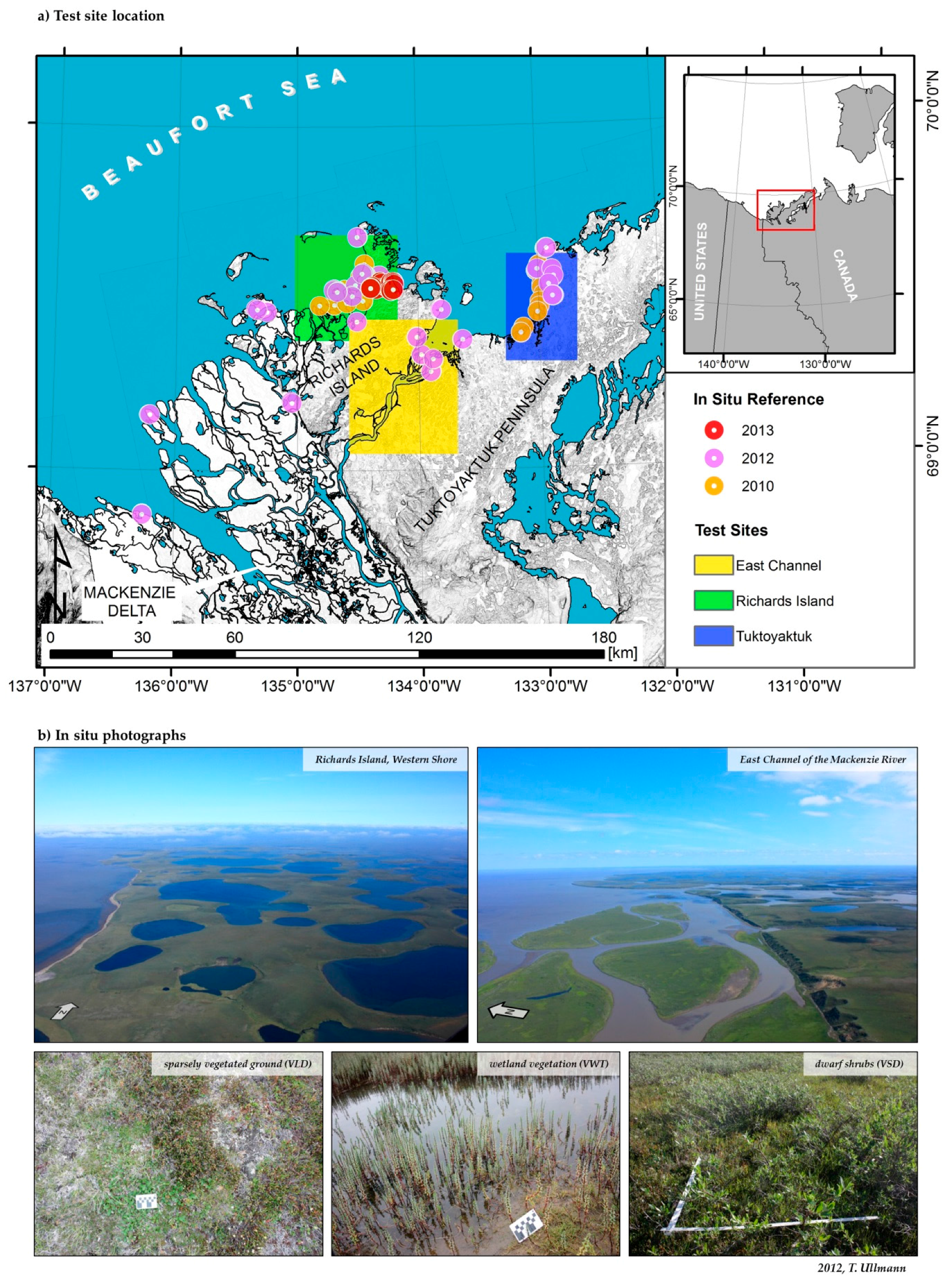
Additionally, in situ ground truth data on the land cover were recorded in the summers of the years 2010, 2012, and 2013. The location of the investigated sites is drawn in Figure 1. In 2010 the field work was conducted by the NWRC (National Wildlife Research Centre, Ottawa, ON, Canada). The field work in 2012 and 2013 was conducted by the Carleton University Ottawa, the NWRC, and the University of Wuerzburg. More than forty locations inside the region were visited and surface properties were documented. The number of reference samples was increased afterwards using high resolution aerial ortho-photos provided by Hartmann and Sachs [34] and NWT-Geomatics [35]. After this operation the set of land cover reference data comprised more than 1700 individual polygons and a minimum of 200 polygons per land cover class. A set of 1000 points per class was then chosen randomly for each test site.

Six land cover classes were distinguished qualitatively in the field (

Table 2. Parameters, description, and scheme of the generalized land cover classes.

Class Name	VWT	NBG	VLD	VMD	VSD
	Wetland	Bare Substrate/Non-Vegetated Ground	Low/Grass and Herb Dominated Tundra	Medium/Mixed Tundra	High/Shrub Dominated Tundra
Scheme
Description	vegetation in standing water dominated by reed and sedge formations	exposed soil substrate and bedrock of varying grain sizes and material	open to closed vegetative cover dominated by formations of grasses, mosses and herbs	closed vegetative cover dominated by formations of herbs and dwarf shrubs	closed vegetative cover dominated by formations of dwarf shrubs and shrubs
Vegetation Height	~10–50 cm	n/a	~5–30 cm	~20–50 cm	~30–100 cm
Shrub Density	n/a	n/a	low	moderate	high

) and in dependence on the classification systems of Corns [36] and the Land Cover Classification LCC-2000-V provided by the authorities of the Natural Resources Canada (geogratis.gc.ca): Water, Bare Ground (NBG), Low/Sparsely Vegetated Tundra (VLD), Medium/Mixed Tundra (VMD), High/Shrub-Dominated Tundra (VSD), and Wetlands (VWT). The main cut-off criteria for the categorization of the land cover classes were the estimated height of the vegetation and the occurrence/density of the shrubs. Table 2 draws the main parameters and a scheme of these generalized land cover classes. The sorting of the classes from NBG to VLD to VMD to VSD corresponds to increasing vegetation height and shrub density on an ordinal scale. Photographs of the classes VLD, VWT, and VSD are provided in Figure 1.

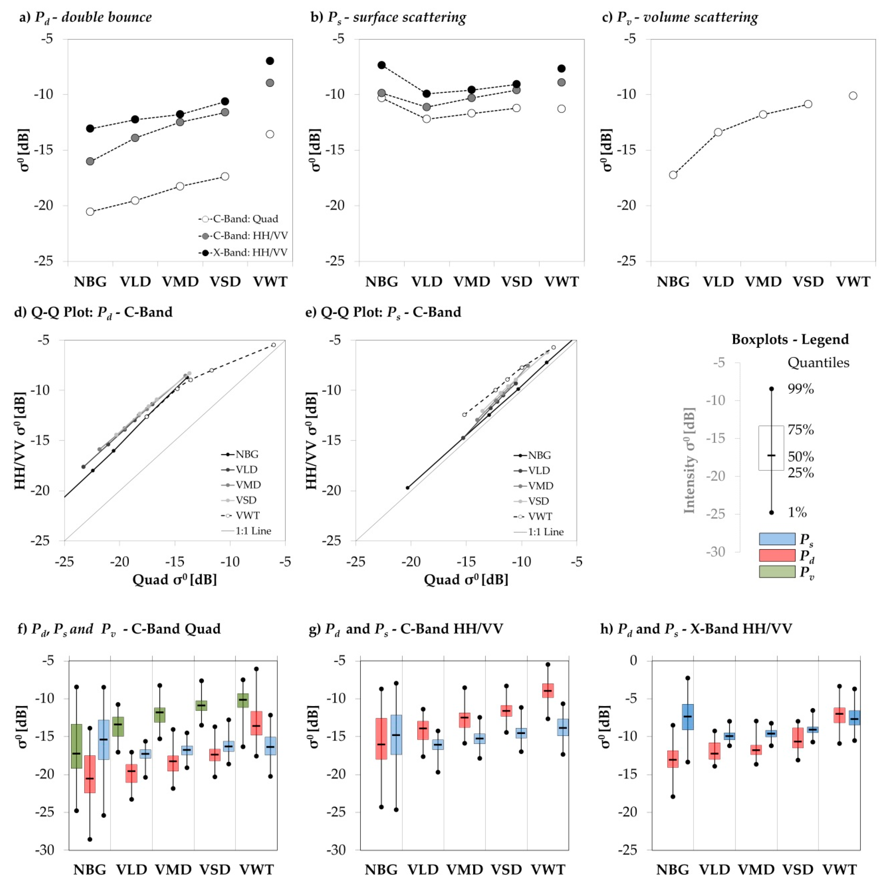
2.4. Correlation Analysis

The relationships and dependencies between the features of the two and three component decomposition were investigated for the C-Band and X-Band datasets using correlation analysis. The two component decomposition features P_s and P_d were processed for C-Band HH/VV-polarized data and X-Band HH/VV-polarized data. The three component decomposition features P_s, P_d, and P_v were processed using the C-Band quad-polarized data. The alterations between the C-Band two and three component decomposition features P_s (P_d) were then connected to the differences of the models and not to changes caused by temporal variations, since pseudo HH/VV-polarized data were derived from quad-polarized data.

Table 3. Decomposition features examined in the correlation, regression, and separability analysis.

Feature	Name	Wavelength	Polarization	Decomposition Model
${\mathrm{P}}_{\mathrm{d}}$	Double Bounce	X-Band	HH/VV	Two Component
${\mathrm{P}}_{\mathrm{s}}$	Surface Scattering	X-Band	HH/VV	Two Component
${\mathrm{P}}_{\mathrm{d}}$	Double Bounce	C-Band	HH/VV	Two Component
${\mathrm{P}}_{\mathrm{s}}$	Surface Scattering	C-Band	HH/VV	Two Component
${\mathrm{P}}_{\mathrm{d}}$	Double Bounce	C-Band	Quad	Three Component
${\mathrm{P}}_{\mathrm{s}}$	Surface Scattering	C-Band	Quad	Three Component
${\mathrm{P}}_{\mathrm{v}}$	Volume Scattering	C-Band	Quad	Three Component

provides an overview of the investigated features.

Prior to the analysis, a random stratification was applied to the land cover reference dataset to avoid auto-correlation: For each land cover class and each test site a set of 1000 pixels was chosen randomly (see Section 2.3 in situ Data).

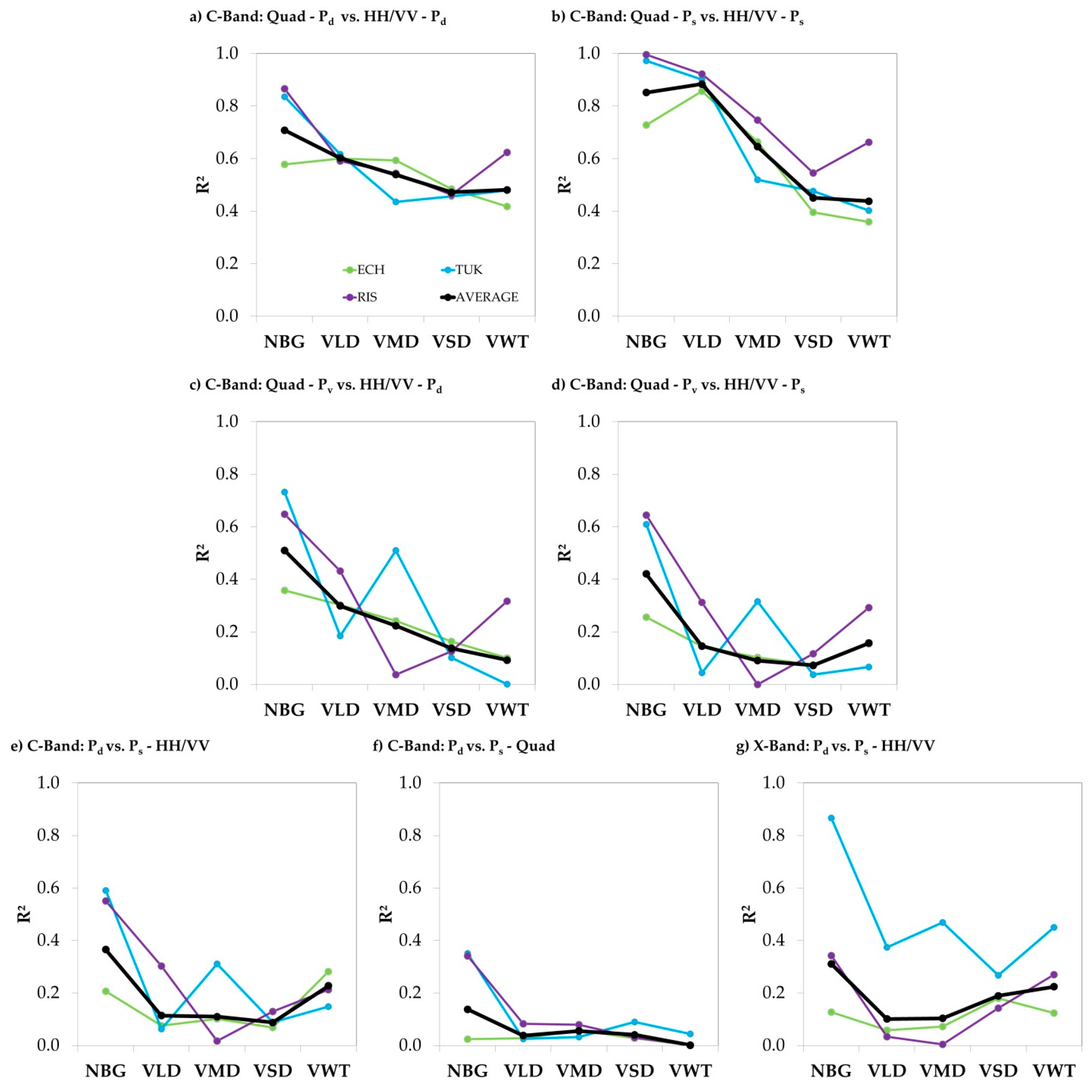
The correlations between the decomposition features were investigated using the intensity values of the sigma nought calibrated data. The linear Pearson Correlation Coefficient (R), the squared linear Pearson Correlation Coefficient (R²), and the Spearman’s Rank Correlation Coefficient ($\mathsf{\rho }$) were processed for all of the features for each land cover class of each test site using the reference data. The coefficient $\mathrm{R}$ is defined as the ratio between the covariance (Cov) of two variables (i,j) and the product of the individual standard deviations of these two variables (SD) (16) and (17). Similar, $\mathsf{\rho }$ is defined as the ratio between the covariance (Cov) of two ranked variables ($R{G}_i,R{G}_j$) and the product of the individual standard deviations of these two ranked variables (${\sigma }_{R{G}_i}{\sigma }_{R{G}_j}$) (18).

$$SD=\sqrt{{\sigma }_i{\sigma }_j}$$

(16)

$$\mathrm{R}=\frac{Cov\left(i,j\right)}{{SD}^2}$$

(17)

$$\mathsf{\rho }=\frac{Cov\left(R{G}_i,R{G}_j\right)}{{\sigma }_{R{G}_i}{\sigma }_{R{G}_j}}$$

(18)

The coefficients R and $\mathsf{\rho }$ are relative and dimensionless and therefore show the linear (R) or monotonic ($\mathsf{\rho }$) correlations among the features, respectively the degree of determination (R²). The values of R and R² range from zero to one, where a value of one (zero) indicates perfect (no) linear correlation and a maximum (minimum) determination, which is 100% (0%) of the explained variance. The values of $\mathsf{\rho }$ range from −1 to +1, where −1/+1 indicate perfect monotonic properties, thus one variable is a function of the other. R and $\mathsf{\rho }$ were investigated to examine the linear and monotonic dependencies among the features. The X-Band data acted as a control variable in this study: A positive correlation between C- and X-Band is expected due to the similar wavelengths of 5 cm and 3 cm, respectively. However; this relationship should be less significant compared to the correlation among the C-Band features due to the temporal decorrelation, the differences in the speckle characteristics, and the differences in absolute radiometric calibration. Therefore it is more statistically reliable to compare C-Band quad-polarized with C-Band synthesized dual-polarized data.

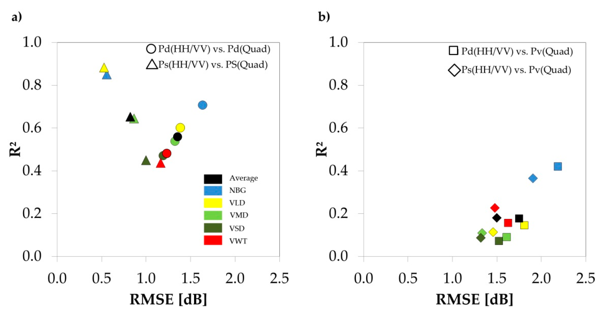
2.5. Regression Analysis

Along with the correlation coefficients, the parameters of the linear regression models were processed for all of the features for each land cover class of each test site using the reference data. The linear model y = ax + b was assumed for the modelling. The two linear model parameters are the slope (coefficient a) and the axis intercept (coefficient b). The differences between the predictions (y) and the true observations (y’) can be expressed via the Root Mean Square Error (RMSE). 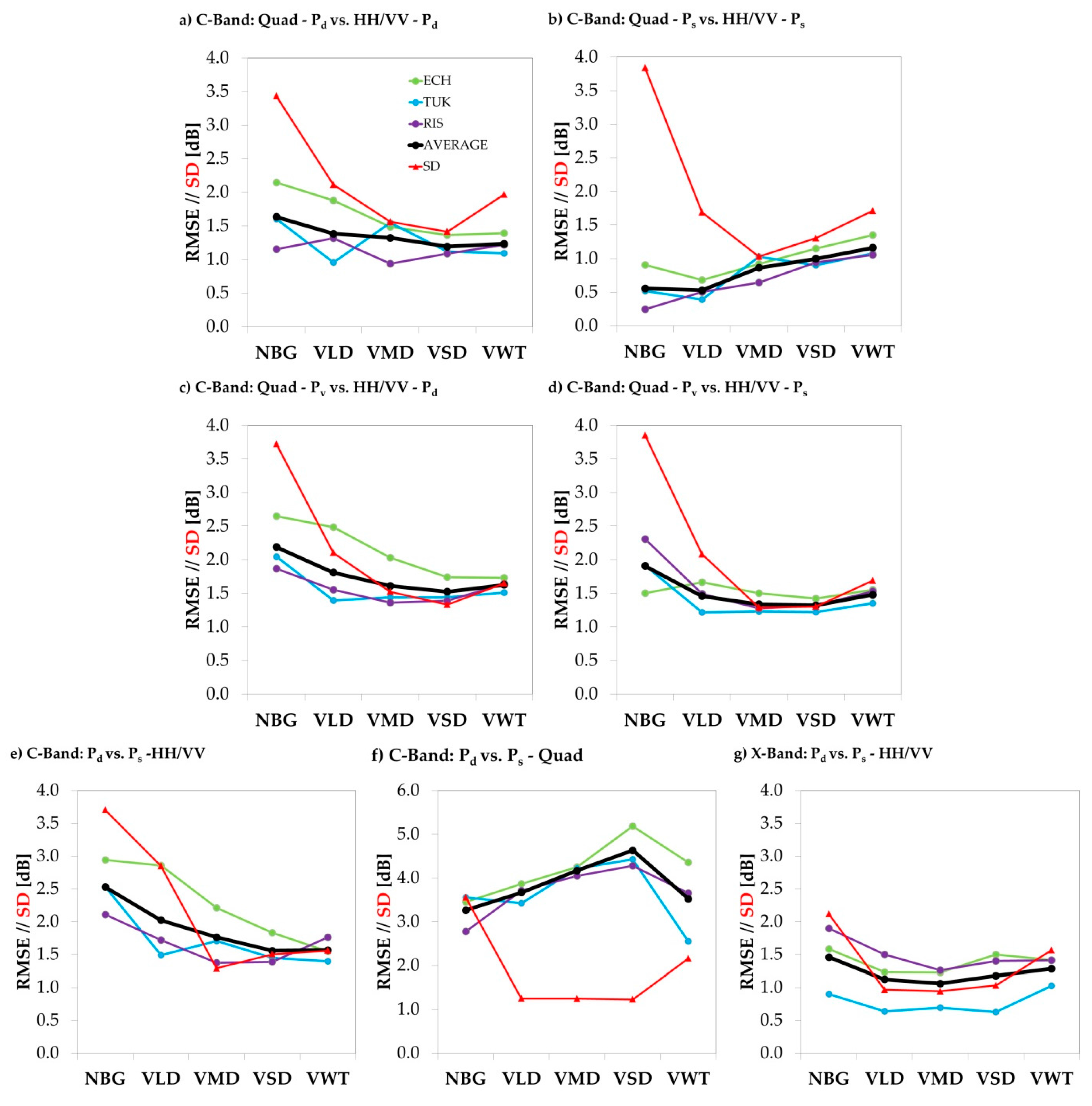The RMSE (Equation (19)) is an absolute measurement of the mean deviation of the model and processed for a sample n. It is therefore measured in the unit of the input variables—decibel (dB) in our case, since the scattering power components were investigated. The RMSE is a frequently used measure to assess the absolute variation of the model prediction, which is often interpreted as the “absolute error” of the model.

$$\mathrm{RMSE}=\sqrt{\frac{{\sum }_{t=1}^n{\left(y_t-{y^{\prime }}_t\right)}^2}{n}}$$

(19)

RMSE is not adjusted to the variances of the two samples (SD) and it should therefore be interpreted along with a relative correlation coefficient, or with a feature that displays the variations of the features (e.g., $SD$). A low (high) coefficient of determination (R²) does not necessarily infer a high (low) RMSE, e.g., in the case that the classes’ standard deviations are low (high).

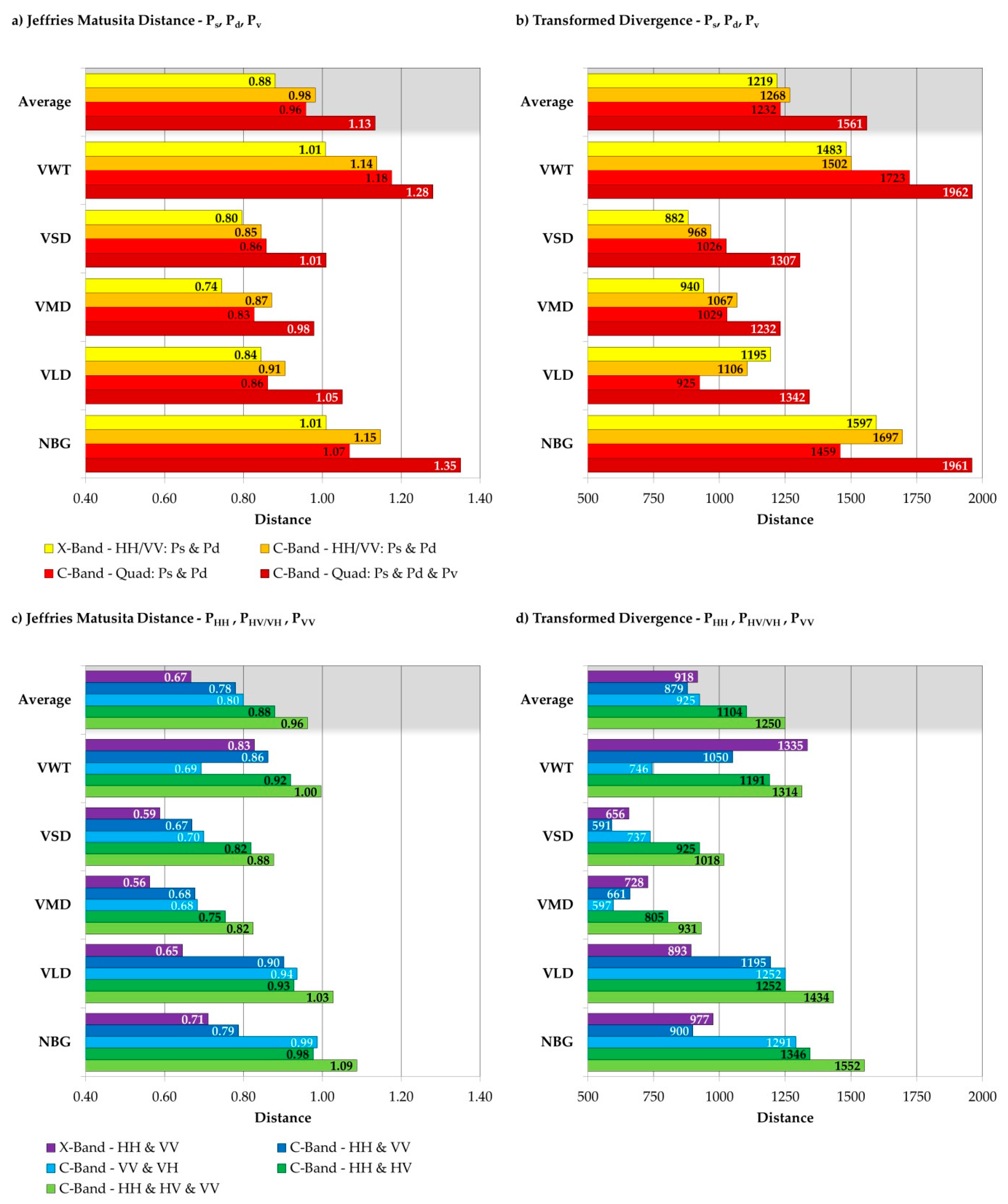
2.6. Separability Analysis

The separability features Jeffries Matusita Distance (JD) and Transformed Divergence (TD) [37,38] were further investigated to examine the differences between C- and X-Band, between the two and three component decomposition features and to examine if PolSAR decomposition offers better class separation compared to the “pure” intensities of the polarimetric channels. The values of the dimensionless JD range from 0.0 to $\sqrt{2}$. The values of the dimensionless Transformed Divergence range usually from 0 to 2000. The higher the value of a separability feature the higher is the estimated separation of the classes in the feature space and the expected classification accuracy. JD and TD require that the values of the classes are normally distributed. This is usually not the case; however a common assumption for natural targets and media for simplicity reasons. JD and TD then estimate the overlap between the multivariate normal distributions of two classes of interest in a given feature space. Less (more) overlap indicates better (worse) separability and therefore the classification accuracy is expected to be higher (lower).

The TD between two classes c and d is defined by Equation (20) using the classes’ mean vectors M and the classes’ covariances V for a given set of features, with two features required as minimum. In the formula tr denotes the trace of a matrix and ^T refers to the matrix/vector transpose. C is a 3 × 3 matrix and M a three-element vector for the case that three features are investigated [37].

$$\mathrm{TD}=2000\left[1-exp\left(\frac{-0.5(tr\left[\left(V_c-V_d\right)\left(V_d^{-1}-V_c^{-1}\right)\right]+tr[\left(V_c^{-1}+V_d^{-1}\right)\left(M_c-M_d\right){\left(M_c-M_d\right)}^T])}{8}\right)\right]$$

(20)

The JD between two classes c and d is defined by (21) and (22) using the classes’ mean vectors M and the classes’ covariances V for a given set of features, with two features required as minimum. The calculation of JD is based on the Bhattacharyya Distance (BD) (21). In the formula det denotes the determinant of a matrix. Both features are based on the Mahalanobis Distance, which estimates the distance between a point and a distribution [37].

$$\mathrm{BD}=0.125{\left(M_c-M_d\right)}^{T}0.5\left(V_c+V_d\right)\left(M_c-M_d\right)+0.5lo{g}_e\frac{det\left(0.5\left(V_c+V_d\right)\right)}{\sqrt{det\left(V_c\right)}\sqrt{det\left(V_d\right)}}$$

(21)

$$\mathrm{JD}=\sqrt{2\left(1-{\mathrm{e}}^{-\mathrm{BD}}\right)}$$

(22)

JD and TD were shown to act as authentic predictors for the accuracy of supervised classifications, when the classifier relies on normal distribution parametrization [37,38,39], e.g., the relationship between JM and supervised classification accuracy obtained from Maximum Likelihood Classification (based on the Mahalanobis Distance). However, the saturation behavior of both features is different and thus it is meaningful to compute and to interpret both in the separability analysis. For this study the land cover reference data were used to define the classes’ statistics. The feature spaces examined were the intensities of C-Band pseudo dual-polarized data (HH/HV; VV/VH; HH/VV), C-Band quad-polarized data (HH/HV/VV), X-Band dual-polarized data (HH/VV), C-Band Three Component Decomposition Features (P_s/P_d/P_v), C-Band Three Component Decomposition Features without the volume scattering (P_s/P_d), C-Band Two Component Decomposition Features (P_s/P_d), and the X-Band Two Component Decomposition Features (P_s/P_d) (Table 3). The analysis was conducted for the none-water land cover classes (NBG, VLD, VMD, VSD, VWT) to avoid an overestimation of the average separability; the class water is comparably easy to be classified with PolSAR data [31] and a high separability of this class might artificially enhance the results.

3. Results and Discussion

3.1. Backscatter Analysis

3.1.1. Results

The backscatter characteristics and descriptive statistics of the land cover classes were investigated prior to the correlation, regression, and separability analyses. Figure 2 shows the medians of the calibrated sigma nought backscatter intensities of the two and three component decomposition features in decibel for each land cover class and the X- and C-Band data. It can be noted that the double bounce intensities P_d are increasing for all features from NBG to VWT (Figure 2a). Contrary, all P_s intensities showed similar value ranges and median values of the vegetation classes (VLD, VMD, VSD) were similar (Figure 2b). The volume scattering P_v of the three component decomposition model showed the most variable value ranges and increasing intensities from NBG to VWT (Figure 2c). P_d and P_v can be considered to be most meaningful for the class characterization and increasing volume scattering, respectively double bounce: The intensities increase with increasing vegetation height and shrub density (from NBG to VLD to VMD to VSD—see Section 2.3 in situ Data).

3.1.2. Discussion

Comparing the features of quad- and HH/VV-polarized data, it can be noted that the characteristics of P_s and P_d of the two and three component decomposition were very similar. This fact is underlined by the quantile-quantile plots (Figure 2d,e). The quantiles of the P_d intensities were comparable and linearly arranged, but showed a bias: The intensity values of the double bounce of the two component model were higher compared to the double bounce intensities of the three component model, which was a result of the volume removal and in the order of 5 dB. The quantiles of P_s were highly related and were located close to the one-to-one line for all of the land cover classes. The bias was small and in the order from 1 to 3 dB. This was especially true for the classes with high P_s intensities. This observation is reasonable since P_s is the sum of the co-polarized channels and the removal of the cross-polarized channel does not alter the signal significantly.

Figure 2f–h and

Table 4. Descriptive statistics—maximum (max), 99% quantile (q99), 1% quantile (q1), minimum (min), mean and standard deviation (sd)—of the investigated features double bounce (P_d), surface scattering (P_s) and volume scattering (P_v) for none-water land cover classes (NBG, VLD, VMD, VSD, VWT) and for C-Band R-2 and X-Band TSX/TDX data. The data show the average of the three test sites Richards Island (RIS), Tuktoyaktuk (TUK) and East Channel (ECH) in the unit decibel (dB).

(a) C-Band (Pseudo HH/VV): Pd						(b) C-Band (Pseudo HH/VV): Ps
	NBG	VLD	VMD	VSD	VWT		NBG	VLD	VMD	VSD	VWT
max	−5.9	−10.1	−6.3	−5.9	−2.8	max	−0.4	−7.9	−5.0	−3.1	−4.2
q99	−8.7	−11.4	−8.5	−8.3	−5.5	q99	−3.0	−9.3	−7.5	−6.2	−5.7
q1	−24.3	−17.6	−15.9	−14.4	−12.6	q1	−19.7	−14.8	−12.9	−12.1	−12.4
min	−24.6	−48.3	−17.6	−48.3	−18.6	min	−21.0	−46.7	−14.9	−46.8	−19.6
mean	−15.7	−14.3	−12.7	−11.6	−9.0	mean	−10.0	−11.4	−10.3	−9.6	−8.9
sd	3.6	2.9	1.5	1.5	1.5	sd	3.8	2.8	1.1	1.5	1.6
(c) X-Band (HH/VV): Pd						(d) X-Band (HH/VV): Ps
	NBG	VLD	VMD	VSD	VWT		NBG	VLD	VMD	VSD	VWT
max	−3.8	−8.4	−7.4	−7.4	0.2	max	2.0	−5.5	−4.5	−4.1	0.5
q99	−8.5	−9.2	−7.9	−8.0	−3.4	q99	−2.3	−8.0	−8.2	−6.5	−3.7
q1	−17.9	−13.9	−13.6	−13.1	−10.9	q1	−13.4	−11.2	−11.2	−10.7	−10.5
min	−18.5	−14.1	−14.3	−14.6	−16.3	min	−17.8	−11.5	−11.8	−14.6	−18.3
mean	−12.9	−11.9	−11.4	−10.3	−7.2	mean	−7.5	−9.9	−9.6	−9.0	−7.5
sd	1.8	1.3	1.4	1.4	1.6	sd	2.4	0.7	0.6	0.8	1.5
(e) C-Band (Quad): Pd						(f) C-Band (Quad): Ps
	NBG	VLD	VMD	VSD	VWT		NBG	VLD	VMD	VSD	VWT
max	−5.2	−15.7	−11.6	−10.5	−3.1	max	−0.8	−9.3	−6.1	−4.0	−5.3
q99	−13.9	−17.0	−14.0	−13.7	−6.1	q99	−3.4	−10.5	−9.4	−7.7	−7.1
q1	−28.6	−23.3	−21.8	−20.3	−17.6	q1	−20.3	−15.3	−14.0	−13.6	−15.2
min	−28.9	−24.6	−23.1	−21.5	−22.0	min	−21.6	−17.3	−16.1	−27.2	−22.2
mean	−20.3	−19.8	−18.4	−17.4	−13.0	mean	−10.5	−12.4	−11.7	−11.2	−11.2
sd	3.3	1.6	1.6	1.3	2.5	sd	3.8	1.0	1.0	1.2	1.8
(g) C-Band (Quad): Pv
	NBG	VLD	VMD	VSD	VWT
max	−7.3	−10.2	−6.5	−3.9	−6.8
q99	−8.4	−10.7	−8.3	−7.6	−7.5
q1	−24.8	−17.0	−15.3	−13.5	−16.3
min	−25.0	−18.8	−17.0	−27.0	−21.9
mean	−16.6	−13.6	−12.1	−10.9	−10.4
sd	3.9	1.5	1.5	1.2	1.8

show the descriptive statistics of the investigated features and underline the aforementioned findings. Two observations are worth noticing here in addition: (1) For the classes VMD, VSD, and VWT standard deviations of all features were less than 2.0 dB. Contrary, the standard deviations of the class NBG ranged between 1.8 and 3.9 dB and were therefore much higher than the standard deviations of the other classes. This fact can be explained by differences in texture (grain sizes) and moisture conditions of different sites that caused a large range of backscatter intensities and therefore a high inter-class variance. The reference data were not suited to investigate these variations in detail; (2) The minimum values of the two component decomposition features of the pseudo HH/VV-polarized C-Band data were very low (<−30 dB) for the classes VLD and VSD, which might be a result of the polarimetric subsetting and of isolated observations with very low intensities in the HH and VV channels.

3.2. Correlation Analysis

3.2.1. Results

Table 5. Average Pearson (a), squared Pearson (b) and Spearman (c) correlation coefficients of C-Band Radarsat-2 and X-Band TerraSAR-X data for two and three component decomposition features double bounce (P_d), surface scattering (P_s), and volume scattering (P_v).

(a) Pearson (R)—Linear Dependence
Pd			Ps			Pv
X-HH/VV	C-HH/VV	C-Quad	X-HH/VV	C-HH/VV	C-Quad	C-Quad
1.00	0.52	0.42	0.20	0.45	0.36	0.47	X-HH/VV	Pd
	1.00	0.83	0.14	0.14	0.10	0.68	C-HH/VV
		1.00	0.10	0.47	0.57	0.35	C-Quad
			1.00	0.14	0.10	0.10	X-HH/VV	Ps
				1.00	0.94	0.64	C-HH/VV
					1.00	0.46	C-Quad
						1.00	C-Quad	Pv
(b) Squared Pearson (R2)—Explained Variance
Pd			Ps			Pv
X-HH/VV	C-HH/VV	C-Quad	X-HH/VV	C-HH/VV	C-Quad	C-Quad
1.00	0.27	0.18	0.04	0.20	0.13	0.22	X-HH/VV	Pd
	1.00	0.69	0.02	0.02	0.01	0.46	C-HH/VV
		1.00	0.01	0.22	0.32	0.12	C-Quad
			1.00	0.02	0.01	0.01	X-HH/VV	Ps
				1.00	0.88	0.41	C-HH/VV
					1.00	0.21	C-Quad
						1.00	C-Quad	Pv
(c) Spearman ($\mathsf{\rho }$)—Monotonic Dependence
Pd			Ps			Pv
X-HH/VV	C-HH/VV	C-Quad	X-HH/VV	C-HH/VV	C-Quad	C-Quad
1.00	0.62	0.53	0.64	0.60	0.49	0.61	X-HH/VV	Pd
	1.00	0.84	0.38	0.67	0.54	0.78	C-HH/VV
		1.00	0.33	0.55	0.48	0.53	C-Quad
			1.00	0.44	0.38	0.39	X-HH/VV	Ps
				1.00	0.91	0.68	C-HH/VV
					1.00	0.51	C-Quad
						1.00	C-Quad	Pv

shows the averaged correlation coefficients between P_s, P_d, and P_v that were derived using the two and three component decomposition models for both X- and C-Band data. For all of the test sites and features positive linear correlations (R > 0) and medium to high positive monotonies ($\mathsf{\rho }$ > 0.3) were observed. The correlations between the X- and C-Band features were very low and the values of the squared Pearson Correlation Coefficients (R²) were less than 0.27. This is most likely a result of the different wavelengths and the temporal gap between the acquisitions. Further, no meaningful correlations between the volume scattering and any other feature were observed: All of the R² values were less than 0.46, which points to the expected statistically independence of the different polarizations. Contrary, the correlation between C-Band surface scattering features P_s of the two and three component models were high (R² = 0.88) and monotone ($\mathsf{\rho }$ = 0.91).

Similarly, the correlation between C-Band double bounce features P_d of the two and three component models were moderately high (R² = 0.69) and monotone ($\mathsf{\rho }$ = 0.84). It is of importance to notice that the correlation between P_d and P_s of the two component model is higher than the correlation between P_d and P_s of the three component model. This fact points to a weaker orthogonality of the features of the two component decomposition model, which appears reasonable due to the missing removal of volume scattering, that is potentially present in both components. In the following the correlation of P_d and P_s between both models was studied for each test site, taking the influence of the land cover into account. Figure 3a,b shows the R² values of the C-Band P_d, and P_s between the two and three component model features for each test site and the average for each land cover class. It was found that the R² values between two and three component P_d (P_s) decreased from NBG to VWT.

3.2.2. Discussion

The decrease in correlation between between two and three component P_d (P_s) is likely due to the increase in volume scattering that was present from NBG to VWT (Figure 2) and a result of the increasing shrub density and vegetation height (Table 2). Thus, the features of the two decompositions were less (more) similar, if the volume scattering contribution was high (low). The drop of the average explained the variance between the classes was up to 0.25 (NBG compared to VWT). Even though this decorrelation was observed, the R² values were still moderate to high for all land cover classes and in average between 0.65 and 0.85 for P_d and between 0.60 and 0.95 for P_s. For further studies it would be of interest to know up to which vegetation height neglecting the volume component within the decomposition is still acceptable and to use only the co-pol scattering coefficients for retrieval of geo-physical parameters. Figure 3c,d shows the correlation between the two component P_d (P_s) and the three component volume scattering P_v. A similar picture was observed and the correlation between the features decreased from NBG to VWT, respectively with increasing shrub density and vegetation height. Contrary to the aforementioned findings, the overall level of the correlation was much lower and ranged between 0.5 and less than 0.1 in average. Thus there was no meaningful direct linear correlation between the two component decomposition features and the volume scattering.

The Figure 3e–g further shows the correlations between P_d and P_s for each model, the land cover classes, and the X- and C-Band data. It was obvious that the three component model facilitated a better orthogonality between P_d and P_s—the correlation between the double bounce and the surface scattering intensities was low and in average less than 0.1; again most likely related to the adjustment of the model to the volume scattering. Contrary, the two component model led to a higher correlation between P_d and P_s intensities which is best pronounced for the HH/VV-polarized X-Band data. However, the R² values of the correlation between P_d and P_s of the two component models were in average less than 0.4 and therefore the features could still be interpreted as rather independent. The two ground components (surface, dihedral) should be orthogonal, depending on the quality of the volume removal and the degree of perfection in scattering type of the two canonical cases (Bragg surface scattering and Fresnel dihedral scattering) [40]. The components should be statistically independent, if both would optimally fit these canonical mechanisms. However, this ideal case might not be observable for real world data.

3.3. Regression Analysis

3.3.1. Results

Table 6. Average linear model parameters: axis intercept (a), slope (b) and Root Mean Square Error (c) of C-Band Radarsat-2 and X-Band TerraSAR-X data for two and three component decomposition features double bounce (P_d), surface scattering (P_s) and volume scattering (P_v).

(a) Linear Model—Axis Intercept—(dB)
Pd			Ps			Pv
X-HH/VV	C-HH/VV	C-Quad	X-HH/VV	C-HH/VV	C-Quad	C-Quad
0.00	−7.84	−9.15	−7.15	−8.74	−9.94	−8.48	X-HH/VV	Pd
	0.00	−3.42	−6.51	−7.19	−9.30	−5.32	C-HH/VV
		0.00	−7.30	−5.98	−15.42	−19.69	C-Quad
			0.00	−6.95	−7.82	−6.92	X-HH/VV	Ps
				0.00	−2.46	−3.87	C-HH/VV
					0.00	−11.05	C-Quad
						0.00	C-Quad	Pv
(b) Linear Model—Slope
Pd			Ps			Pv
X-HH/VV	C-HH/VV	C-Quad	X-HH/VV	C-HH/VV	C-Quad	C-Quad
1.00	0.23	0.09	0.44	0.20	0.08	0.18	X-HH/VV	Pd
	1.00	0.49	0.17	0.58	0.32	0.59	C-HH/VV
		1.00	0.08	0.20	0.32	−0.10	C-Quad
			1.00	0.18	0.08	0.14	X-HH/VV	Ps
				1.00	0.64	0.47	C-HH/VV
					1.00	0.16	C-Quad
						1.00	C-Quad	Pv
(c) Linear Model—Root Mean Square Error (RMSE)—(dB)
Pd			Ps			Pv
X-HH/VV	C-HH/VV	C-Quad	X-HH/VV	C-HH/VV	C-Quad	C-Quad
0.00	1.38	1.44	1.24	1.41	1.45	1.38	X-HH/VV	Pd
	0.00	1.78	1.45	1.85	2.22	1.85	C-HH/VV
		0.00	1.48	2.10	3.87	3.87	C-Quad
			0.00	1.45	1.47	1.44	X-HH/VV	Ps
				0.00	1.05	1.64	C-HH/VV
					0.00	2.19	C-Quad
						0.00	C-Quad	Pv

shows the results of the linear regression modelling and draws the averaged parameters slope, axis intercept, and the RMSE for P_s, P_d, and P_v derived from the two and three component decomposition models for both X- and C-Band data. The interpretation of the axis intercept and the slope of the model is difficult, since no perfect one-to-one relation between the features of the two and three component models can be assumed due to the differences in the total backscattered energy between quad- and dual-polarized data and the C- and X-Band data, respectively. We observe that P_d and P_s of the two component models are biased by approximately 2 to 3 dB compared to P_d and P_s of the three component model. This is also evident from the quantile-quantile-plot in Figure 2. Table 6(c) further indicates the average RMSE error between the P_d and P_s of C-band two and three component model. The RMSEs are comparably low and less than 2 dB, thus underlining that the absolute model error is estimated to be low and a prediction seems therefore reliable.

3.3.2. Discussion

However, more meaningful is the interpretation of the RSME along with the results of the correlation analysis and depending on the type of coverage and the volume scattering. Figure 4a,b shows the RMSE values of the C-Band P_d and P_s between the two and three component model features for each test site and the total average for each land cover class.

The graphs further show the product of the standard deviations of the two variables (SD) for each land cover class. At a first glance the results are non-intuitive: RMSE between the C-Band two and three component model feature P_d decreases from NBG to VWT and therefore the model error decreases with increasing volume scattering intensities, which is the opposite to our expectations. However, the reason for this observation is the weak linear correlation between the features for the vegetation classes (Figure 3a). Therefore the RMSE becomes a function of the standard deviations of the two variables (SD; see Section 2.4 Regression Analysis), as it is obvious in the graph (compare Table 4 as well). Thus, the behavior of the RMSE can be explained by the SD values, which is also true in Figure 4c–f and partially in Figure 4a for the classes VMD, VSD, and VWT. Figure 5 shows the observations of Figure 3 and Figure 4 in a scatterplot. The RMSE is drawn on the abscissa and the explained variance (R²) on the ordinate. This plot summarizes the findings made in the aforementioned sections.

Figure 5a indicates that the values of three and two component decomposition are generally highly correlated (R² > 0.8) with low RMSE (RMSE < 1 dB) for the surface scattering intensities P_s and for classes with no (NBG), respectively low vegetative coverage and vegetation height (VLD). It is further observed that the correlation between P_d of three and two component model is generally lower and RMSE is higher compared to the findings made for the P_s. Figure 5b graphically summarizes the results of the previous analyses: the correlation between the two component model features and the three component volume scattering is low and the RMSEs were high and in average lager than 1.5 dB, while R² was in average less than 0.2.

3.4. Separability Analysis

3.4.1. Results

In the following the effect of two and/or three component decomposition on the separability of classes in the feature space was investigated (see Section 2.6 Separability Analysis). Figure 6 shows the results of the assessment for the non-water land cover classes. Figure 6a,b displays the results obtained with polarimetric decomposition. Figure 6c,d displays the results obtained without polarimetric decomposition—that means that only the intensities of the polarimetric channels were used in the separability analysis. The results are further displayed for the JM (left side) and the TD (right side); however, differences between JD and TD were small and restricted to individual classes and feature combinations.

3.4.2. Discussion

In summary the following findings concerning the separability were made: (1) the polarimetric decomposition generally increased the separability of the land cover classes in the feature spaces. This was true for the two and the three component decomposition. It is therefore worth processing the decomposition features in order to obtain higher classification accuracy; (2) X-Band HH/VV-polarized data realized lower separability compared to the C-Band HH/VV-polarized data; however, results were not clear due to general low values of TD and JD.

Anyway, this assessment suggested that C-Band HH/VV-polarized data were better suited for the land cover characterization than X-Band HH/VV-polarized data. (3) Among the possible dual-polarization modes (HH/HV; VV/VH, and HH/VV) the HH/VV data were shown to be best suited, if the two component decomposition was used. The HH/HV, followed by the VV/VH and the HH/VV, was best suited, if just the polarimetric channel intensities were used. This underlined the high value of the HH/VV data and the meaningfulness of polarimetric decomposition as well as the application of polarimetry as observation space, respectively; (4) The volume scattering intensity, extracted via polarimetric decomposition of quad-polarized data, was shown to be best suited for the separation of the examined tundra land cover classes. The separations offered in combination with the surface scattering and double bounce intensities were much higher than the separabilities offered by any other feature combination; (5) The capability of PolSAR for the classification of the examined tundra land cover classes was especially high for non-vegetated ground and wetland vegetation. The discrimination of vegetation classes, like shrub dominated tundra, was generally limited, low accuracies should be expected in land cover classification, and involving the cross-polarized information is recommendable with a view to the assessment. Among all examined feature combinations the cross-polarized component was crucial to achieve good separability between the vegetation classes.

3.5. Example—Test Site Tuktoyaktuk (TUK)

3.5.1. Results

Figure 7 illustrates the findings of the analyses for a subset of the test site TUK. The Figure 7a,c,d shows the P_d (double bounce), P_s (surface scattering), and P_v (volume scattering) intensities of the three component decomposition derived from C-Band quad-polarized data. The Figure 7b,e shows the double bounce (P_d) and surface scattering (P_s) intensities of the two component decomposition derived from C-Band HH/VV-polarized data. All data are displayed as calibrated sigma nought intensities in decibel. The legend in the lower right corner of the figure lists the minimum and maximum values used for the linear stretch (grayscale). Figure 7f shows the RGB color composite of the three component decomposition features with R = P_d, G = P_v, and B = P_s. It indicates as well the dominating land cover units along the profile line (A → B): low/sparsely vegetated tundra (VLD), wetland (VWT) and shrub dominated tundra (VSD). It is obvious that the class VSD caused a higher volume scattering, which is pronounced in the volume scattering feature (Figure 2c)) via higher intensities and with greenish color in the RGB composite (Figure 7f). The class VWT is characterized by high intensities in the double bounce of the two and three component model (Figure 7a,b). The high intensity further caused a reddish color in the RGB composite (Figure 7f). This is a result of the water to vegetation (double bounce) scattering, the interaction of the wave with the water surface and the vegetation body, respectively. The class VLD indicates medium high intensities in all of the features and it shows up in blueish color in the RGB composite (Figure 7f). Additionally, Figure 7g displays the intensities values of P_d of two and three component model along the profile line (A → B). The intensities are strongly related and show the same peaks and troughs. The influence of the land cover on the double bounce intensities is clearly visible: The wetland vegetation (VWT) causes higher backscatter intensities compared to the other land cover classes, most likely due to dominant dihedral scattering. Both P_d features show similar value ranges and identical intensities for some locations.

The differences between both datasets are bigger for the low tundra (VLD) and maximized for the shrub dominated tundra (VSD). Figure 7h shows the scatterplot of two and three component P_d of the profile values. Two clusters are visible, one very close to the one-to-one line and a second cluster that is slightly biased: Nevertheless, a clear positive and linear dependency is visible (overall R² = 0.75). Figure 7i illustrates the profile values of P_s of two and three component model. Again both lines are related and showed the same peaks and troughs and similar value ranges. Contrary to the observations made for the double bounce, the wetland vegetation (VWT) caused maximum differences between both features.

The higher backscattering intensities of P_s of the two component model are most likely related to the missing removal of the volume scattering contribution and differences are in the order of 5 dB. The alterations between P_s of the two and P_s of the three component model are lower for the shrub dominated tundra (VSD) and minimized for low tundra coverage (VLD). For the class named last the profile values are nearly identical aligned and differences between the features of both models are small.

3.5.2. Discussion

The intensities of the two and three component models showed nearly identical values due to low intensities of the cross-polarization (low volume scattering contribution). Figure 3j shows the scatterplot of two and three component P_s of the profile values. As observed for the P_d, two clusters were recognizable and a positive dependency was visible, however it was less strong (overall R² = 0.40). The cluster closer to the one-to-one line corresponds to the samples of the land cover class VLD (high determination, R² = 0.66), the more scattered samples to VWT and VSD (lower determination, R² < 0.6). Finally, Figure 7k shows the volume scattering intensity P_v of the three component model. The shrub dominated tundra (VSD) showed the highest volume scattering intensities. The value ranges of the low tundra (VLD) and the wetland (VWT) were comparable and lower than the value range of VSD (−2 to −7 dB). This example made two points clear: First, the double bounce (surface scattering) intensities of both models were closely related for the classes VWT (VLD). For both land cover types VLD and VWT low volume scattering intensities were present (−10 to −17 dB). Second, differences between them were maximized for the land cover class VSD that showed higher volume scattering (−5 to −10 dB).

4. Summary and Conclusions

This research study investigated a two component decomposition model for HH/VV-polarized PolSAR data. The proposed approach decomposes the total backscattered energy into two features that represent the intensities of surface and double bounce scattering. The used model is a straight forward adaptation of the decomposition model of [29]; however, it does not involve the cross-polarized information. The dependencies between two component features, derived from HH/VV-polarized data (X- and C-Band), and three component features, derived from quad-polarized data (C-Band), were investigated for the tundra environment of the Mackenzie Delta Region, Canada. Several PolSAR acquisitions of Radarsat-2 (Quad) and TerraSAR-X (HH/VV) were available for the summer months of the years 2010, 2011, and 2012. Additionally, in situ ground truth data on generalized land cover units were collected in 2010, 2012, and 2013. The land cover reference was used threefold: First, the backscatter characteristics of each PolSAR feature were analyzed for the land cover classes. Second, the correlations and regressions among the HH/VV- and quad-polarized features were investigated using the Pearson Correlation Coefficient (R) and the Spearman Rank Correlation Coefficient and the Root Means Square Error (RMSE) of the linear model. Third, the separability of the classes in the feature spaces of two and three component decomposition of X- and C-Band data were investigated and compared to the separability offered by the intensities of the polarimetric channels. The following main findings are reported:

(1)

The features of two and three component decomposition scattering components (surface, dihedral) showed similar backscatter characteristics for the examined land cover classes and therefore provided a similar interpretation. The distributions of the features double bounce and surface scattering of the two and three component model were shown to be very similar in the quantile-quantile-plot and the average bias was less than 5 dB for the double bounce and less than 3 dB for the surface scattering.

(2)

In average, the correlation between the double bounce features of the two and three component model showed R² values around 0.69. The R² values observed for the surface scattering features of the two and three component model were around 0.88. Thus, the decomposition features of HH/VV-polarized (derived as polarimetric subset from the quad-polarized data) and quad-polarized data were similar and positively correlated. The RMSE of the linear model was in average less than 2 dB for both features.

(3)

The presence of volume scattering led to differences between the two and three component decomposition intensities and these differences were maximized when the volume scattering contribution was high. This was indicated by the analysis of the regression and correlation coefficients. The R² values between double bounce, respectively surface scattering, intensities of the two and three component decomposition model were high for land cover classes that cause the least volume scattering, e.g., bare or sparsely vegetated ground, and were around 0.7 to 0.9 for the double bounce and 0.6 to 0.8 for the surface scattering. The R² values were low for land cover classes that caused high volume scattering, e.g., shrub dominated tundra or wetland vegetation. The observed R² values were then in the order from 0.4 to 0.5.

(4)

The correlation between double bounce and surface scattering intensities of the two component model was higher (R² < 0.4) than the correlation between the double bounce and surface scattering intensities of the three component model (R² < 0.2). Thus, the two component model realizes a weaker orthogonality of the features, which is a result of neglecting the cross-polarized information and the removal of an existing volume component—depolarization acts on surface, as well as, on dihedral scattering component in terms of roughness.

(5)

The volume scattering intensity of the three component decomposition model showed the highest sensitivity to the land cover classes and provided the best separability among the classes, as indicated by the assessment of the separability features, Jeffries Matusita Distance (JM) and Transformed Divergence (TD). Therefore, the quad-polarized data offered in average a better separation than the co-polarized data due to the benefit of having the cross-polarized information. Therefore the quad-polarized data will be better suited for the classification of the examined tundra land cover types. However; the land cover classes of wetland vegetation, bare ground, and low tundra showed clear positions in the feature space of the HH/VV-polarized data and an accurate classification of these land cover types is likely to be done with such dual-polarized SAR data: The JM and TD were highest among the possible dual-polarization modes (HH/VV; HH/HV; VV/VH) and HH/VV was found to be the favorable mode for the characterization of the named land cover classes. The HH/HV-polarized and VV/VH-polarized data were found to be best suited for the characterization of mixed and shrub dominated tundra as indicated by the separability analyses.

(6)

None of the HH/VV-polarized features showed a direct linear correlation with the volume scattering, respectively with the cross-polarized information, which is expected in terms of physics causing independence of the two polarimetric scattering types.

The application of the analyzed two component decomposition generated polarimetric features (scattering type components) that facilitated the interpretation of the dual-polarized SAR signal and these features were found to be useful to categorize the type of scattering and to characterize the tundra land cover in the investigated area. The proposed decomposition model is not adjusted to distinct vegetation cover with a significant volume contribution, due to the missing incorporation of the cross-polarized information in the decomposition model. This has to be considered when interpreting the features and when relating the type of backscatter to the land cover. For C- and X-Band data an application of the purposed decomposition is therefore advantageous for the characterization of the natural land coverage and therefore for low (Arctic) vegetation that cause a low volume scattering contribution, e.g., sites of bare or sparsely vegetated ground. Further, the characterization and classification of wetlands is likely to be done with the HH/VV-polarized data. Investigating such natural land coverage, the HH/VV data and its decomposition features will serve as a reliable substitute for the double bounce and surface scattering features of the three component decomposition model of quad-polarized data.

Upcoming research should address the following issues: (1) Application of the decomposition model for other Arctic and non-Arctic sites and investigation on model transferability; (2) Application of the synthetic cross-polarization as an intermediate step between no volume information for HH/VV dual-polarization and full cross-polarized information (quad) [10,41,42]. Along with this the application of other dual-polarization decompositions, e.g., the eigen-decomposition, or the Kennaugh-Matrix decomposition [43], should be investigated; (3) Realization of land cover classifications for Tundra environments with PolSAR data, potentially including also multi-spectral data [26]; (4) Analysis of the decomposition model with time series in order to investigate the temporal behavior of the tundra land cover in terms of scattering mechanisms, e.g., for the determination of the phenological response, freeze and thaw cycle (e.g., [44]), or moisture conditions.