1. Introduction
1.1. Global Food and Agriculture
There is a need to double output of agricultural systems by 2050 to meet the increasing food demands from a growing global population; forecasted to peak at 9.22 billion by 2050 [
1,
2]. Wheat continues to provide the sole vital daily nutrition for 35% of the world’s population [
3] and is therefore a key focus of yield improvement research.
Projects such as the 20:20 Wheat
® project at Rothamsted Research, aim to provide the knowledge and tools to increase the UK’s wheat yield potential to 20 tonnes of wheat per hectare within 20 years [
4], whilst combating the new challenges agriculture is facing such as climate change. These projects focus on developing new improved varieties through methods such as selective breeding.
Key to this is the monitoring of different varieties for favourable genotypes and phenotypes, by providing a continuous stream of data documenting the course of the crops development and responses to environmental conditions [
5,
6].
1.2. Phenotyping
Phenotyping of crops involves the measurement and assessment of physical observable characteristics [
7]. Current phenotyping techniques particularly the capacity to collect quality repeatable phenotypic data in field representative growing conditions is a bottleneck for further advancements in knowledge and development of crop varieties and yield gains [
8].
Height may be a useful indicator of yield, carbohydrate storage capacity and susceptibility to lodging [
9,
10] as well as being an essential parameter for site-specific management practices [
11]. Monitoring crop height during development stages is a reflection of cultivar and growing conditions. Crop development stages are often defined by the Zadoks Scale [
12,
13], and in terms of crop growth and height changes the key period of growth in UK grown wheat occurs between the start of stem elongation in early April, stage GS30, and anthesis in mid-June, stage GS61. Anthesis, or flowering, is the point at which crop height is considered to be at maximum [
14]. Whilst exact timings of specific development stages will vary between cultivars, it is an important that any method of measuring crop height is able to accurately measure height during all stages between GS30 and GS61 where vegetative structure can vary.
1.3. Measuring Height
Crop height is classified as the shortest distance between the upper boundary of the main photosynthetic tissues on a plant and the ground level [
15,
16]. Most commonly height data is collected with a measuring rule [
10] which although simple, is both laborious, inefficient and can introduce a level of subjectivity into data collected. Applying this method over large trial fields, totalling upwards of 1000 plots, limits the repeatability of this method.
There is a need for rapid, precise, continuous and in-season acquisition of this data [
17] in order to better understand external, environmental influences throughout the crops development cycle. Current methods are not sufficient to meet this need, in particular for use in crop trials where the number of measurements required is large and as such development of new technologies and methods is needed.
Within this paper, we introduce and investigate quantitatively the method of Structure-from-Motion (SfM) photogrammetry using high resolution Unmanned Aerial Vehicle (UAV) imagery to accurately model crop trials, from which generation of crop heights can be calculated.
1.4. UAVs in Research
Unmanned Aerial Vehicles (UAVs), also referred to as Unmanned Aerial Systems (UAS), are a growing technology that is rapidly gaining popularity in both the public and scientific communities. UAVs offer a customisable aerial platform from which a variety of sensors can be mounted and flown to collect aerial imagery with very high spatial and temporal resolutions. Advancements in the accuracy, economic efficiency and miniaturisation of many technologies including GPS and computer processors has pushed UAV systems into a cost effective, innovative remote sensing platform.
Of most significance for research applications is the gap which this technology fills in the remote sensing domain. UAVs overcome the restrictions of resolution and cost that often hamper the use of satellite and airborne remote sensing respectively. The wide variety of sensors which can be mounted and flown over a predetermined area, means an almost endless list of possible applications for this technology.
A review of the literature highlights the wide range of applications UAVs and mounted sensors have been utilised for. For environmental monitoring, examples include modelling of the temporal changes in landslide dynamics [
18]; 3D reconstruction of fluvial topography of UK streams [
19]; monitoring of rangeland [
20,
21] and conservation applications such as surveying of habitats and animal numbers [
22]. Alternatively, UAVs have been applied in documenting of archaeological sites, where the rapid collection of very high-resolution 3D reconstructions from UAV based methods has been proven useful [
23]. In terms of agriculture, UAVs have been used for the monitoring of water status and drought stresses in fruit trees [
24]; additionally, collecting multispectral and hyperspectral imagery for use in spectral indices [
25] and even chlorophyll fluorescence [
26].
1.5. Structure-from-Motion and Crop Modelling
SfM photogrammetry is an emerging method that offers high resolution 3D topographic or structural reconstruction from overlapping imagery [
27,
28]. Key to SfM methods is the ability to calculate camera position, orientation and scene geometry purely from the set of overlapping images provided, offering a simple processing workflow compared to alternative photogrammetry techniques [
29,
30]. The simple and easy workflow of SfM for generating 3D digital reconstructions of landscapes or scenes makes it applicable for use a variety of research fields as well as in agricultural crop monitoring.
A number of studies have applied UAV based SfM to modelling crop heights and/or growth over the growing season. Bendig et al. [
31,
32] applied UAV based SfM methods to model and calculate heights of barley and rice crops in the field. Results showed room for development in the methods and technologies used; comparisons with ground measured heights of barley produced regression coefficients values of 0.55, 0.22 and 0.71 on three different dates. The authors highlight issues with GPS accuracy as a main source of crop height error, as well as suggesting using higher quality cameras for image collection. Ruiz et al. [
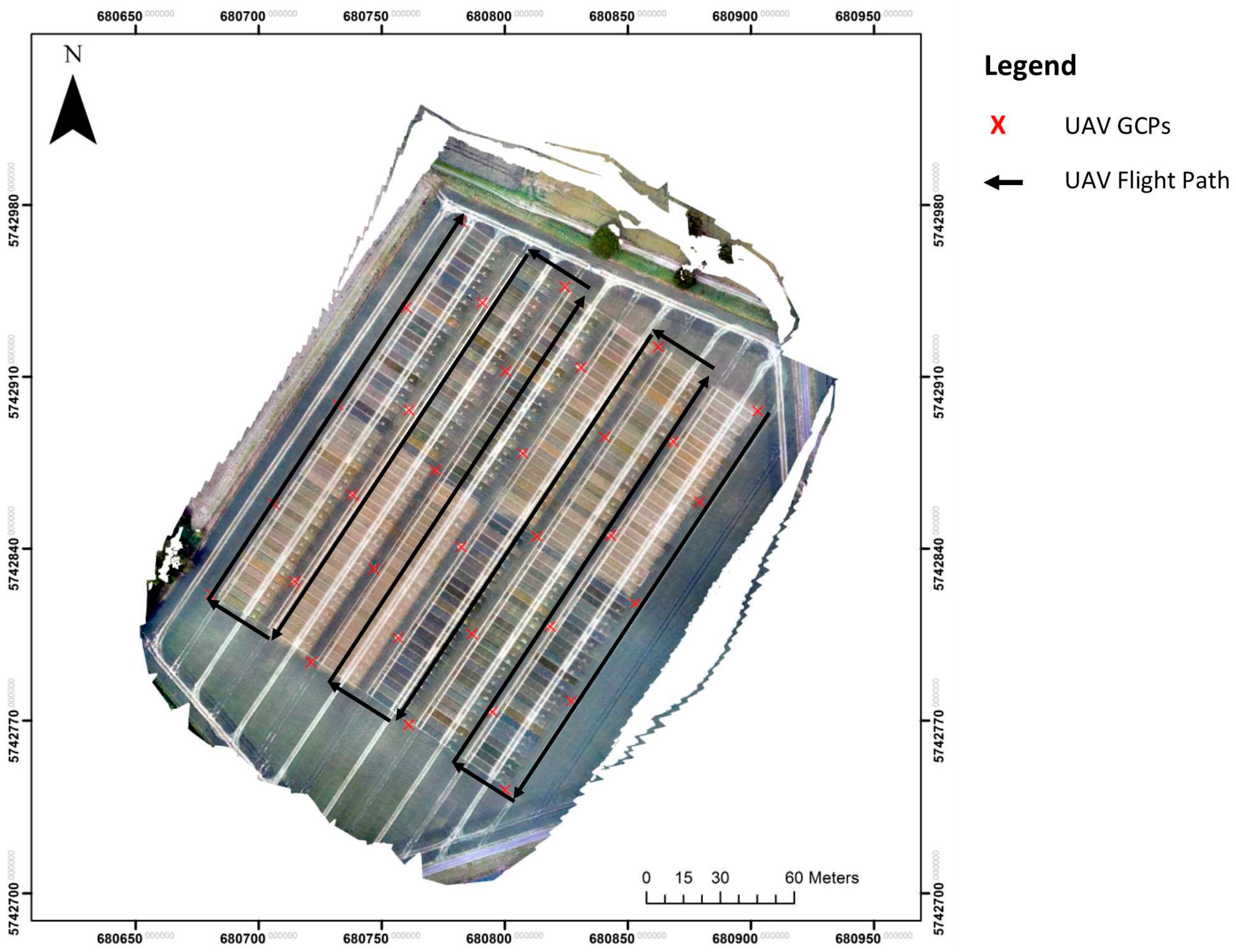
33] also found the SfM algorithms suffer from errors present in GPS datasets. Ground-based Control Points (GCP) located within the scene are recommended as best-practice for spatial accuracy and minimisation of model error. Turner et al. [
34] found GCPs offered a significant improvement in spatial accuracy compared to directly georeferenced imagery using the UAVs on-board GPS. Aasen et al. [
35] used hyperspectral imagery collected from a UAV for vegetation monitoring including height. Results from this study were found to be comparable with others (R
2 = 0.7) with a consistent underestimation of plant height by 0.19 m. The authors highlight the fact that the rule has its own issues when it comes to accuracy and therefore may not offer the best source of ground validation. However, as the standard procedure currently in practice, rule measurements still hold a level of importance when proving the validity of UAV based SfM methods.
Image resolution is particularly important for early season crop modelling where the lack of closed canopies impacts on “Crop Surface Model (CSM)” production [
36]. Higher resolutions offer a good level of improvement in model accuracy. Willkomm et al. [
37] generated models with spatial resolutions of 0.5 cm, with height reconstructions comparable to the other studies discussed (R
2 = 0.75) and point out a tendency of the UAV models to underestimate heights. Interestingly the authors highlight the inability to isolate singular plant details within the model due plant movement during acquisition, likely due to wind. There is a potential that this crop movement, caused by windy conditions, and subsequent loss of some plant structures may be the cause of the underestimation of the model.
The review of relevant literature has shown UAV based SFM is applicable to modelling of plant heights however accuracy of models achieved in these studies highlights improvements are needed. It is clear that a proof of concept has been achieved, however the development of this concept into a working procedure applicable to real world agricultural research is now the next step.
The aim of this study is to produce a highly accurate and repeatable method for collecting crop heights from UAV based Structure from Motion Photogrammetry models as an alternative to current manual rule based phenotyping methods.
The research will involve accuracy assessments and comparisons with alternative technologies, method development and full season testing of the SfM technique. A full quantitative assessment will address the following research questions:
How accurate are the models and crop heights generated, compared to the rule method; the existing industry standard?
How replicable is the method over the development cycle of wheat crops, particularly between stages GS30 and GS61 (Zadoks Scale); can growth be monitored?
Can these methods be applied in crop research and does it offer a better quality of data compared to the rule method?
4. Discussion
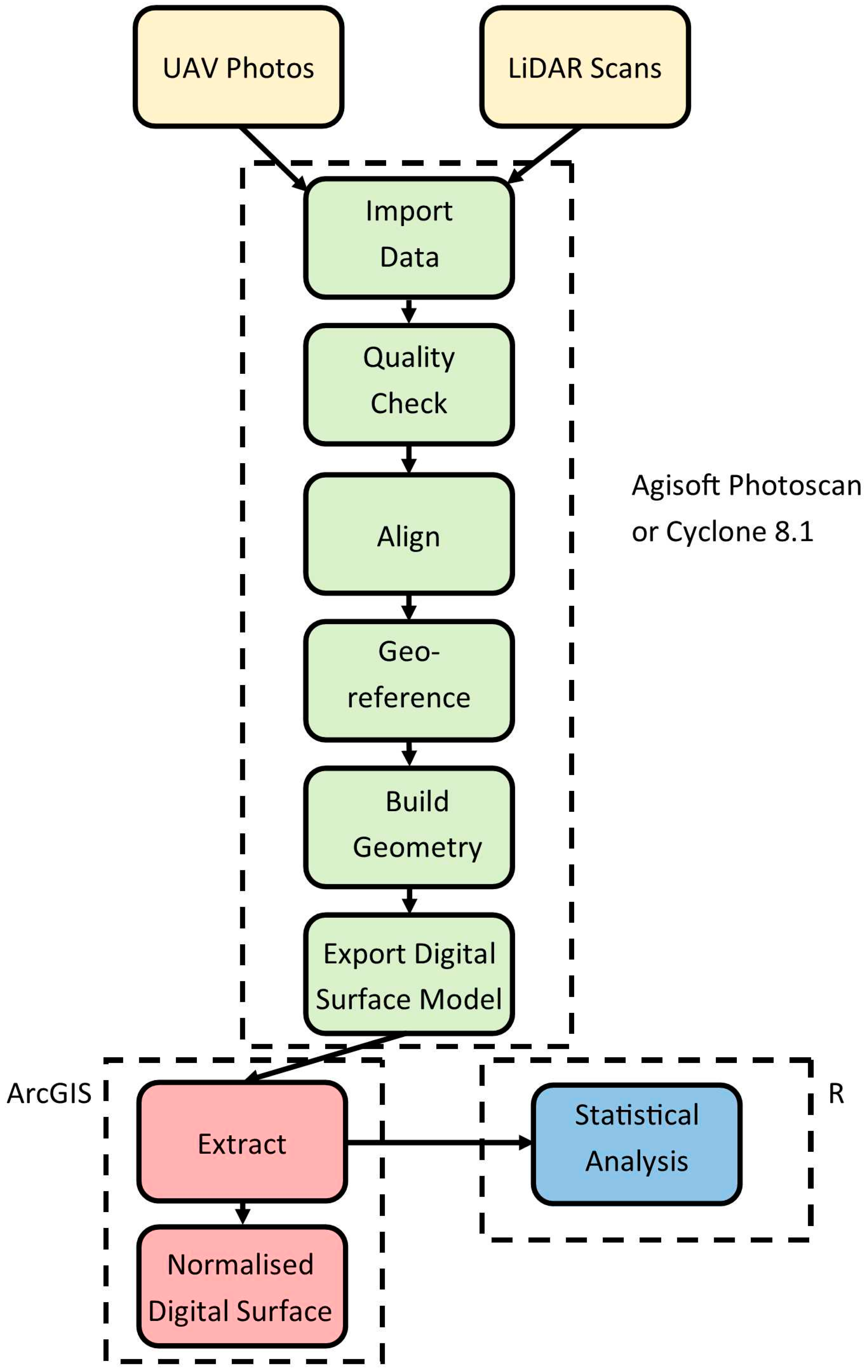
This study has provided a quantifiable assessment of Unmanned Aerial Vehicle (UAV) based Structure from Motion (SfM) Photogrammetry for deriving accurate measurements of crop height and crop growth rate, in this case to support field phenotyping efforts of 25 wheat varieties grown under four different nitrogen fertiliser treatments. The method presented is relatively straightforward, easily repeatable, and time and cost efficient in comparison to the terrestrial LiDAR and currently used rule method also investigated in this study.
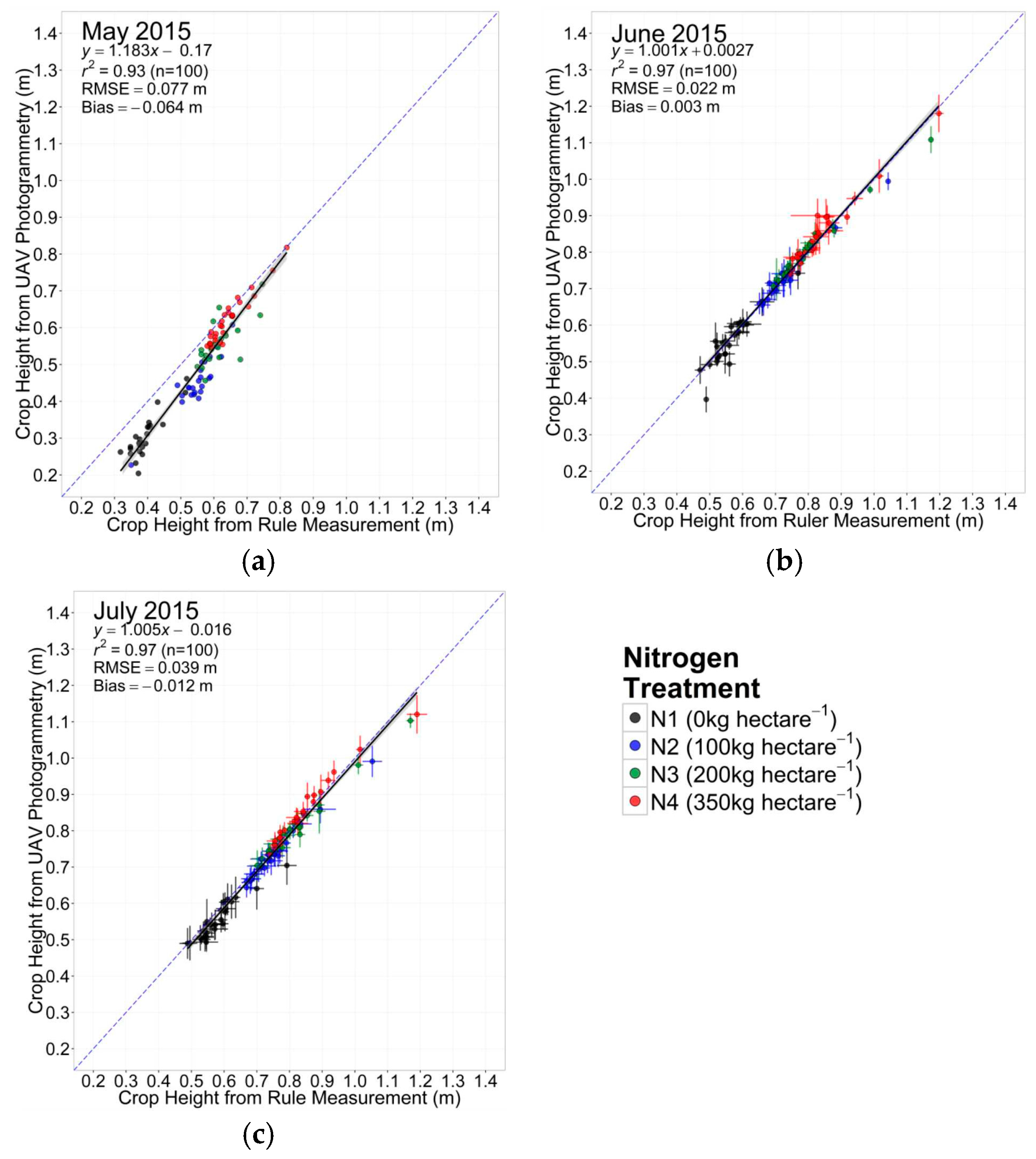
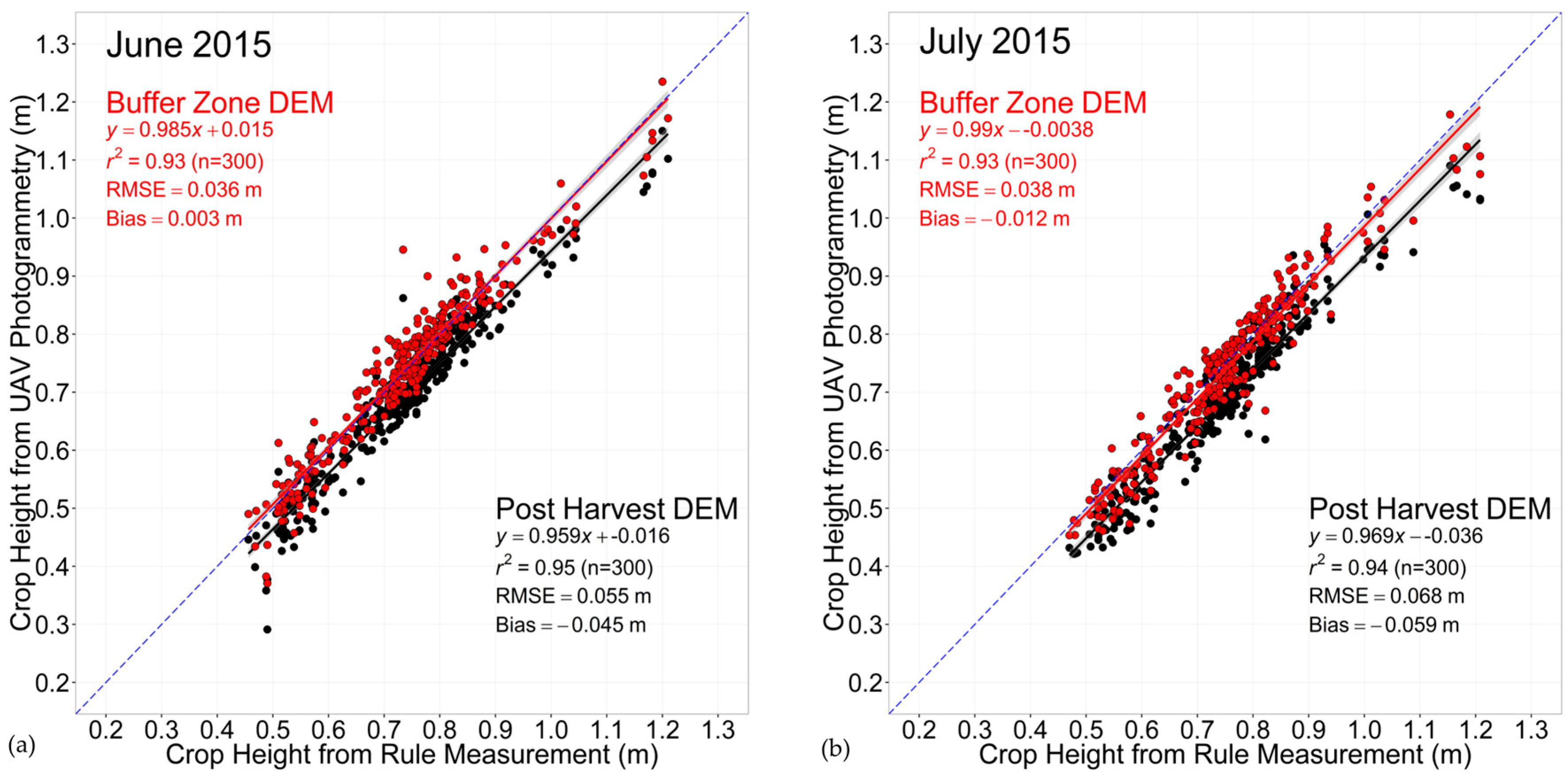
In terms of accuracy, the data produced provide good agreement with the currently applied procedure of manual measurement with a rule (R2 = ≥0.93, Root Mean Squared Error (RMSE) = ≤0.077 m) but this approach is more consistent and spatially extensive, reducing user error associated with the ruler measurement [
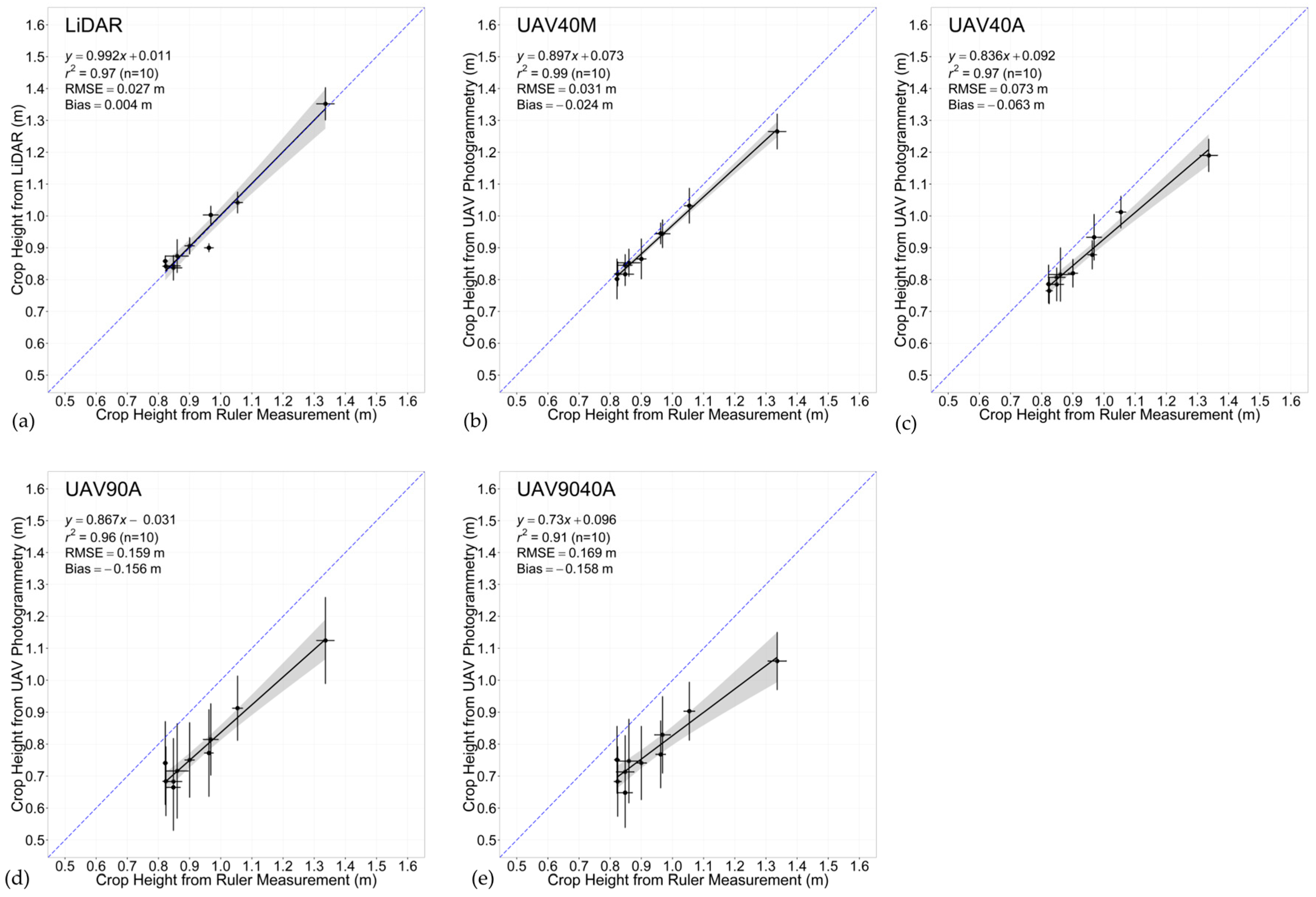
35,
44]. Assessment of model derived crop heights from a highly accurate (5 mm) Terrestrial LiDAR (R2 = 0.97, RMSE = 0.027 m) and the best UAV model (R2 = 0.99, RMSE = 0.03 m) shows both system’s ability to produce highly accurate results; however extremely high costs and poor time efficiency of the LiDAR due to the high number of individual scans required, severely lower the suitability of LiDAR for this application. The UAV method was found to often underestimate crop heights, as discussed by previous studies [
35,
37], but overall the results showed an improvement in accuracy compared to similar studies [
31,
32,
45], even when the method was applied over a significantly larger number of trial plots (300).
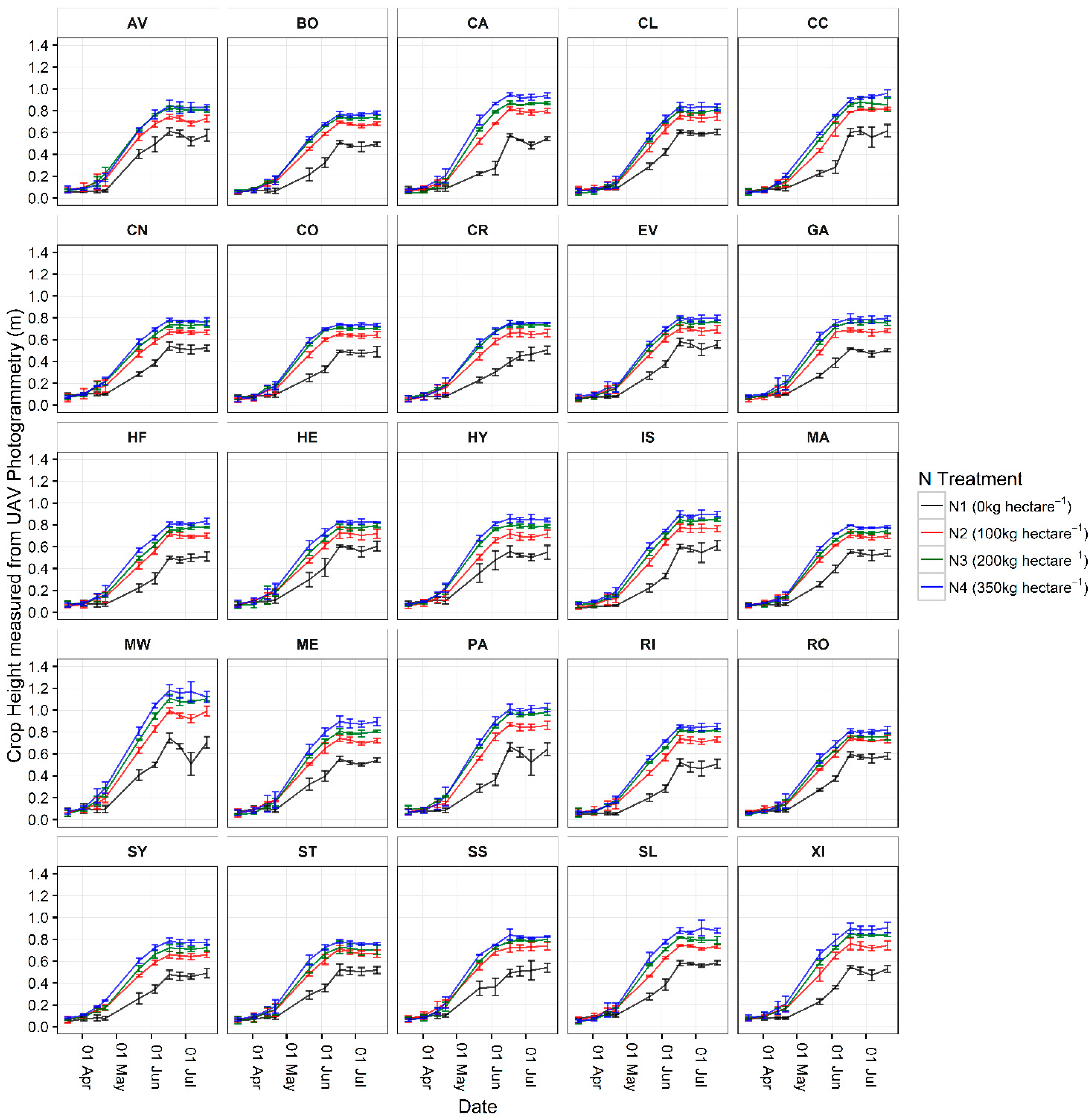
Collection of crop heights over the growing season has proven the ability of this method to collect valuable phenotypic data at development stages between GS30 and GS61 (Zadoks Scale), and is in agreement with literature [
31,
46]. A number of field based variables were identified from the study as key influencers on final results; namely canopy structure and density were found to impact on model height accuracy both in early growth stages and in crops grown under nutrient deficient conditions, as also discussed by [
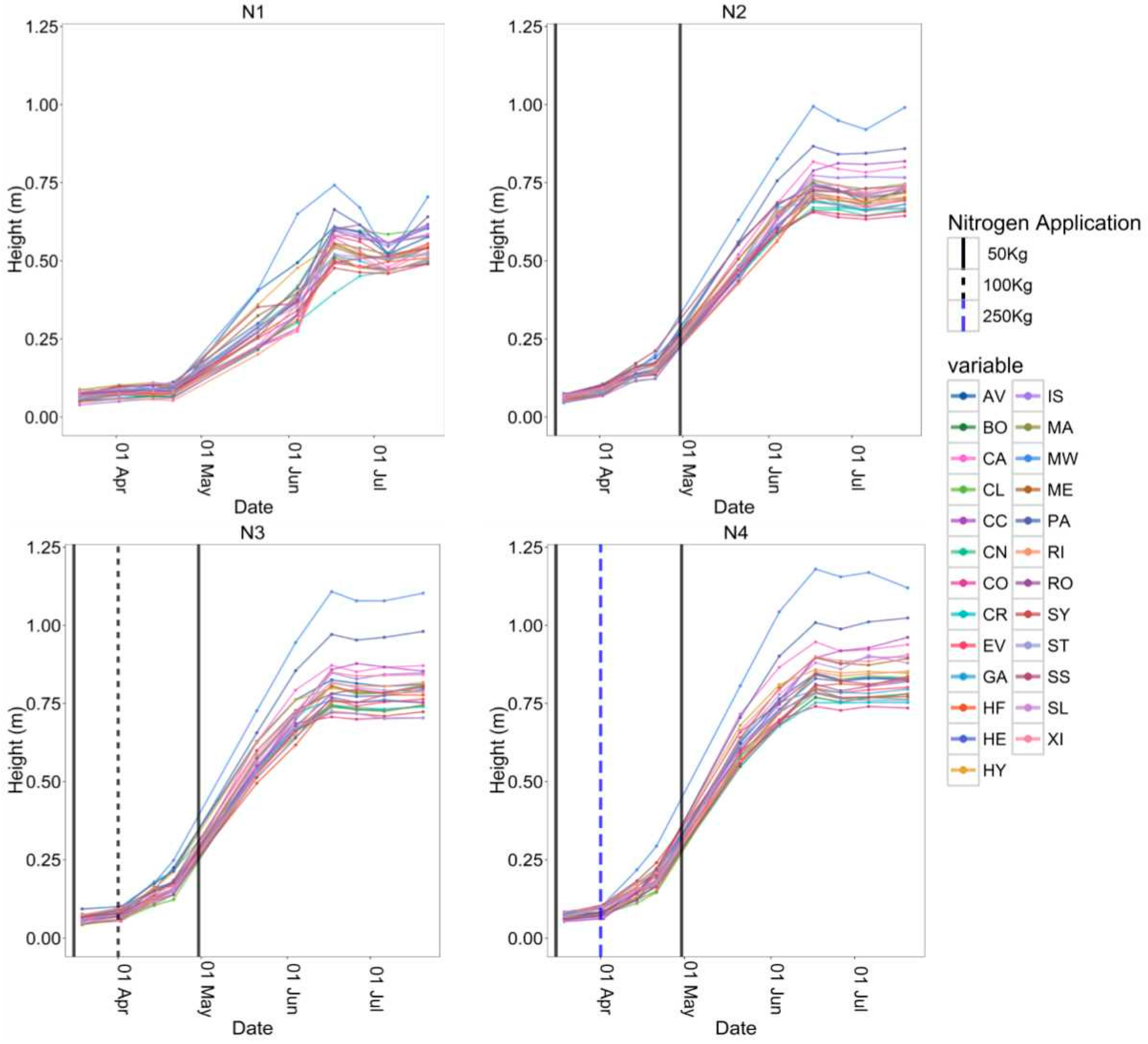
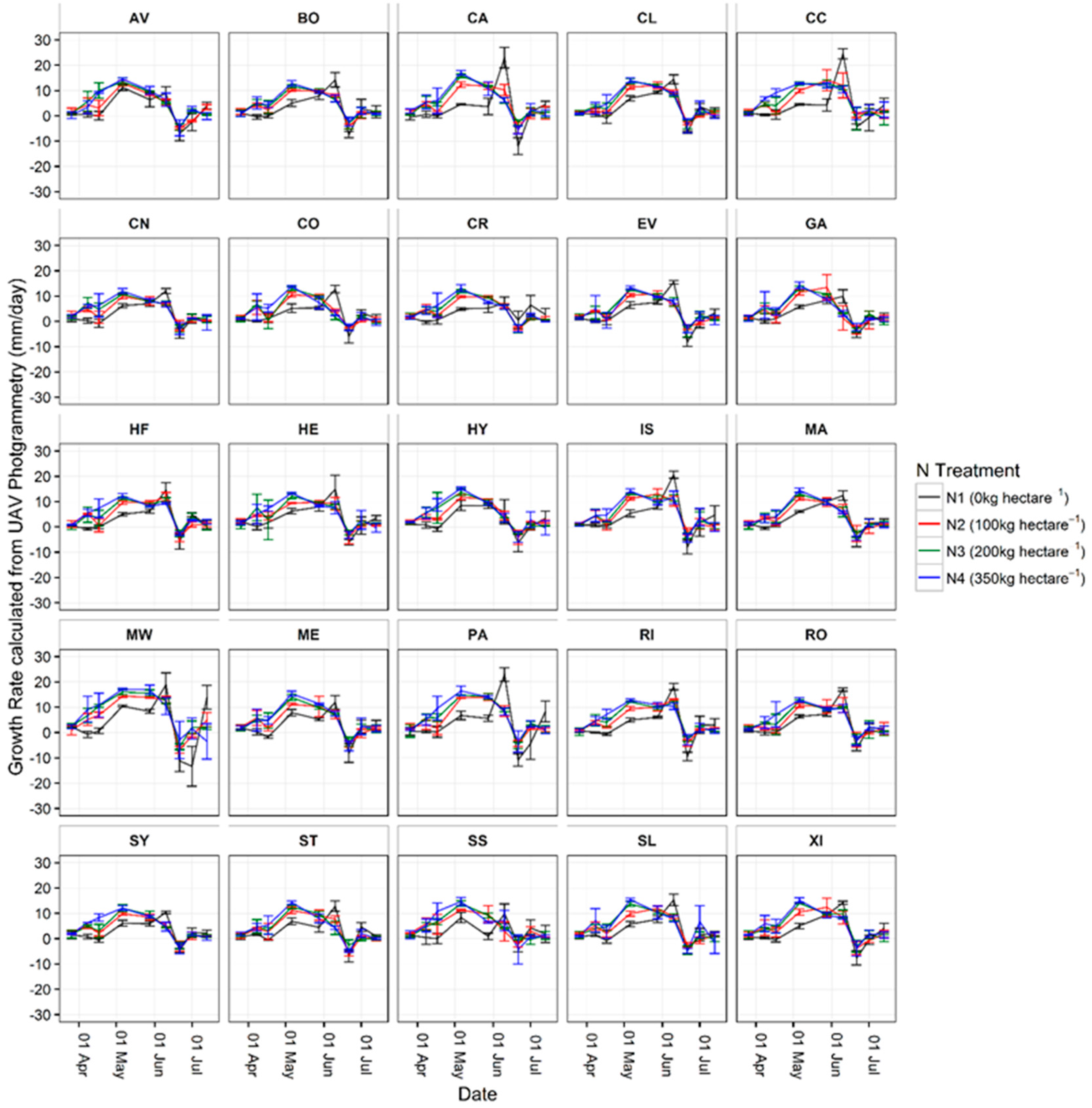
36]. The repetition of height measurements from the UAV method allowed crop growth rates to be calculated and assessed. The main results of this study were in agreement with the literature which defines the main period of UK wheat crop growth in terms of height gain between early-April and mid-June [
14].
As a high-throughput field phenotyping system, this study has demonstrated that UAV SfM is capable of collecting quality, high volume field based phenotypic data. Comparison to the LiDAR shows the UAV method is able to achieve the same high level of accuracy whilst bettering the LiDAR in terms of time and cost efficiency. Alternative high-throughput platforms that have been developed and investigated further show the value of a system for rapid monitoring of canopy dynamics; such as the Field Scanalyzer [
47] as well as movable tractor based systems [
48,
49]. Advantages of these systems over the UAV focus strongly on the lack of weight restrictions, allowing for multiple sensors to be used to collect very high resolution data from multiple sensors simultaneously. However, these systems are limited in their application over larger areas, or across different field locations, something the UAV is better suited to. The tractor based system proposed by Comar et al. [
49], was able to sample ~100 plots per hour, which equates to 1000 plots within three days assuming 4–5 h of measuring per day. The UAV method was able to cover 300 plots within a single flight of maximum 15 min, indicating coverage of 1000 plots could be achieved in less than an hour. Clearly there is a trade-off between the systems discussed here as well as other alternatives. The choice of which system is most suitable will be dependent on the data required, the time frame available and the area of coverage needed.
Whilst the method developed in this study has been shown to produce quality results over the temporal scale of a growing season, there is still room for improvement in the understanding of SfM photogrammetry dependencies. For example, in relation to the camera viewing angle, James and Robson [
29] found the inclusion of oblique imagery into a NADIR image data set can further improve 3D model accuracy. In this study, software settings were also found to be influential on accuracy of model outputs, therefore in future these should be carefully selected and accurately reported in order to facilitate further advances in UAV based SfM methods and in the accuracy of results. The use of NIR imagery instead of RGB is also an area of interest, as the increased contrast between plant and soil offered by NIR imagery may improve model processing; a potential solution to the negative influence of decreased canopy structure on model derived heights as shown by the May accuracy assessment results (
Figure 10) and also discussed in the literature [
36].
5. Conclusions
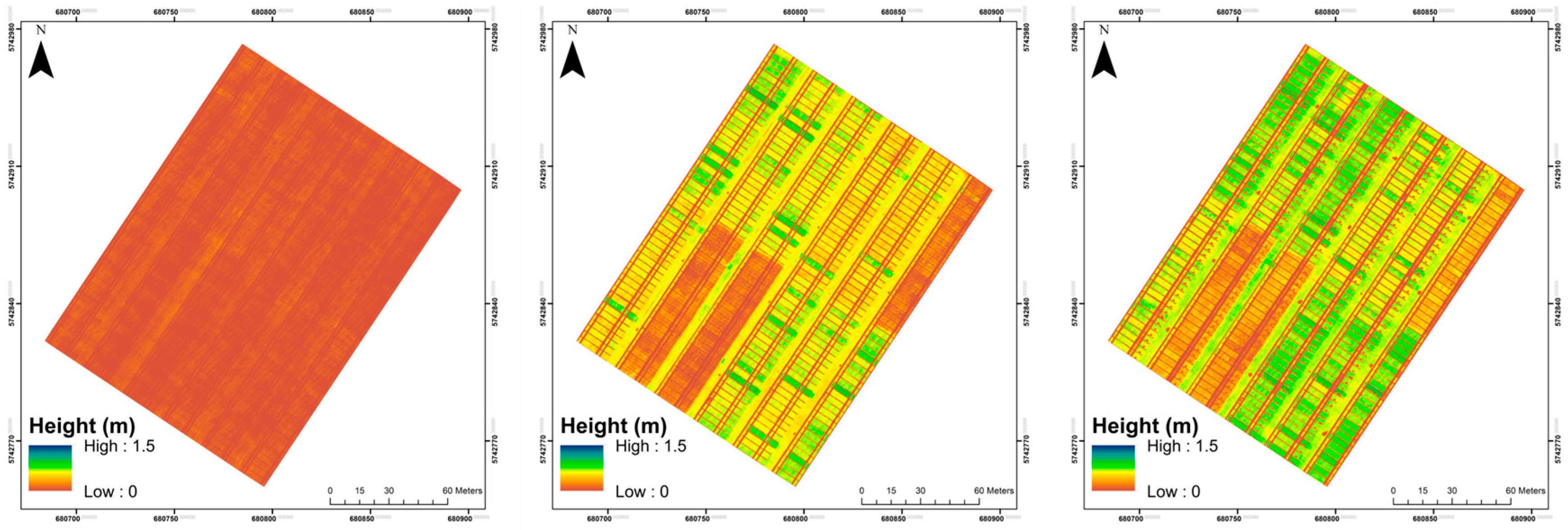
The work presented in this paper develops a rapid and accurate method for collecting in-field measurements of crop height using Unmanned Aerial Vehicle (UAV) based remote sensing. The UAV method developed utilises very high resolution UAV imagery and a Structure from Motion photogrammetry workflow to produce 3D topographic reconstructions of the crop trial field. Accuracy assessments of the UAV derived crop heights showed the method was able to produce measures of height comparable in accuracy to those measured by the existing manual, rule based method (R2 = ≥0.92, Root Mean Squared Error (RMSE) = ≤0.07m). The very high spatial resolution of the UAV derived data allows for assessment of spatial variability in crop height at both the field and plot scale. UAV flight campaigns throughout the season allowed for the monitoring of changes in crop height as well as the calculation of growth rate.
Future work will look to increase the temporal resolution of the methods in order to provide a more complete picture of this phenotypic trait throughout the development stages of the different cultivars. It will also look to develop methods using other imaging equipment such as multi-spectral [
50,
51,
52], hyper-spectral [
35] and thermal cameras [
53,
54] to provide information beyond just plant height and growth rate. This should help to open up the opportunity to collect a more complete set of crop phenotype metrics at a spatial and temporal resolution usually unavailable to plant scientists, offering greater insights into varieties behaviours and adaptability under different growing conditions.
Overall, UAV SfM has the potential to become a valuable tool for rapid high-throughput in-field phenotyping of crop heights at very high resolution and accuracy for use in crop trials or more general agricultural applications.


 and
and 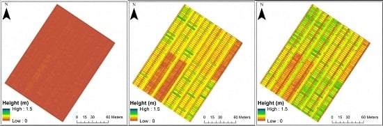


