
Enhancing Noah Land Surface Model Prediction Skill over Indian Subcontinent by Assimilating SMOPS Blended Soil Moisture

Abstract
:
1. Introduction
2. Materials and Methods
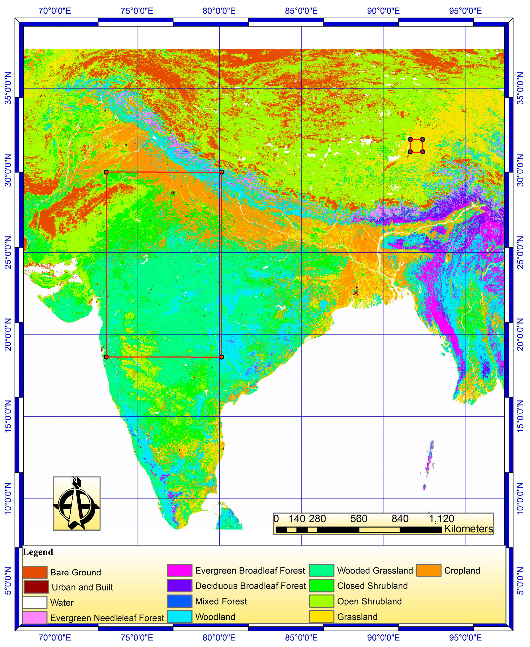
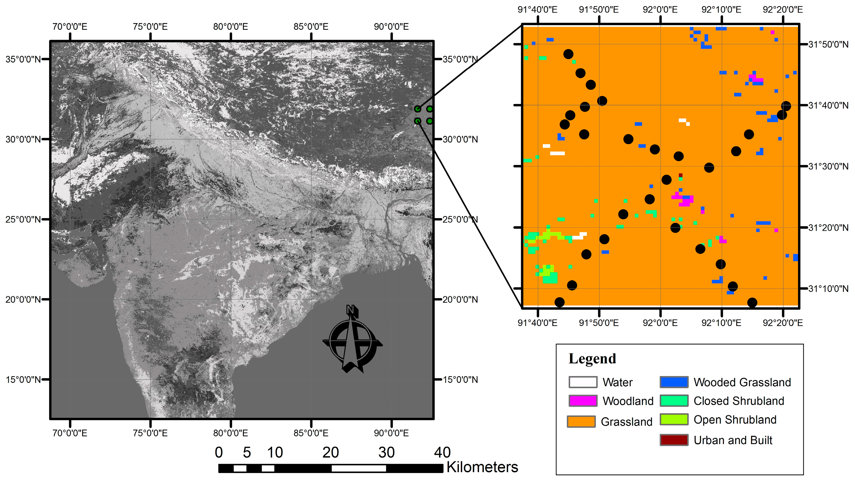
2.1. Study Area
2.2. The Land Parameter Retrieval Model (LPRM) AMSR-E Soil Moisture
2.3. SMOPS Blended Products
2.4. Global Data Assimilation System (GDAS)
2.5. Ecoclimap
2.6. ISMN Ground Data for Tibetan Plateau
2.7. Land Surface Model Framework
LSM Spin-up
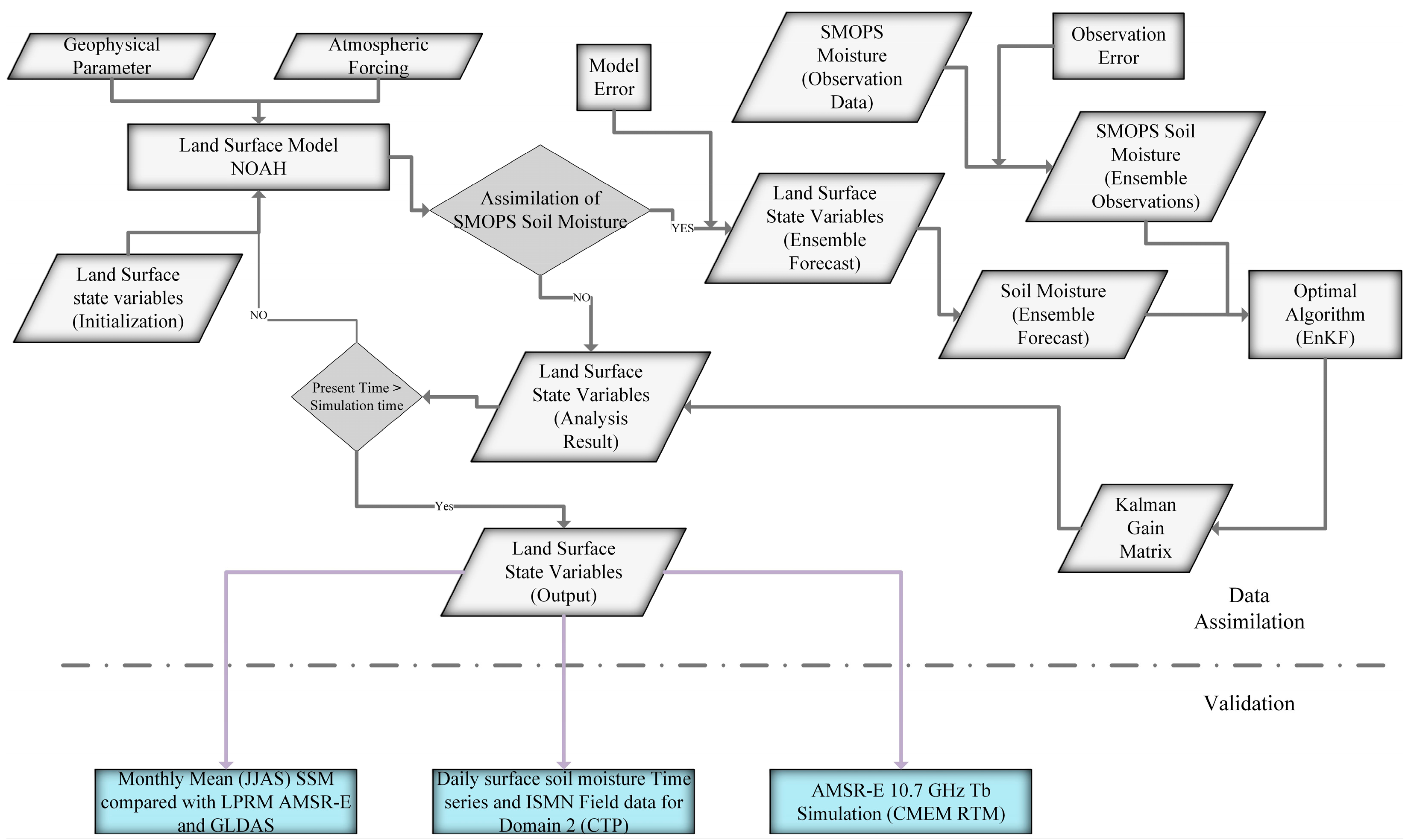
2.8. Data Assimilation Framework
2.8.1. Ensemble Kalman Filter
2.8.2. Perturbation Attributes
2.9. Radiative Transfer Model
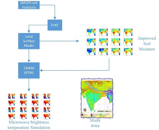
3. Study Setup
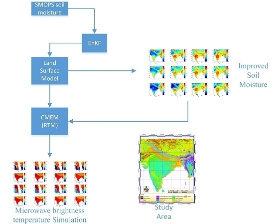
3.1. Study Overview
- (a)
- Data assimilation, where the Noah LSM was initialized with spinup runs(explained in Section 2.7), and then the initialized model was assimilated with SMOPS soil moisture by using NASA’s LIS framework for 0.25° × 0.25° spatial resolution with the procedure as shown in Figure 3. A similar procedure was used by Kumar et al. [43].
- (b)
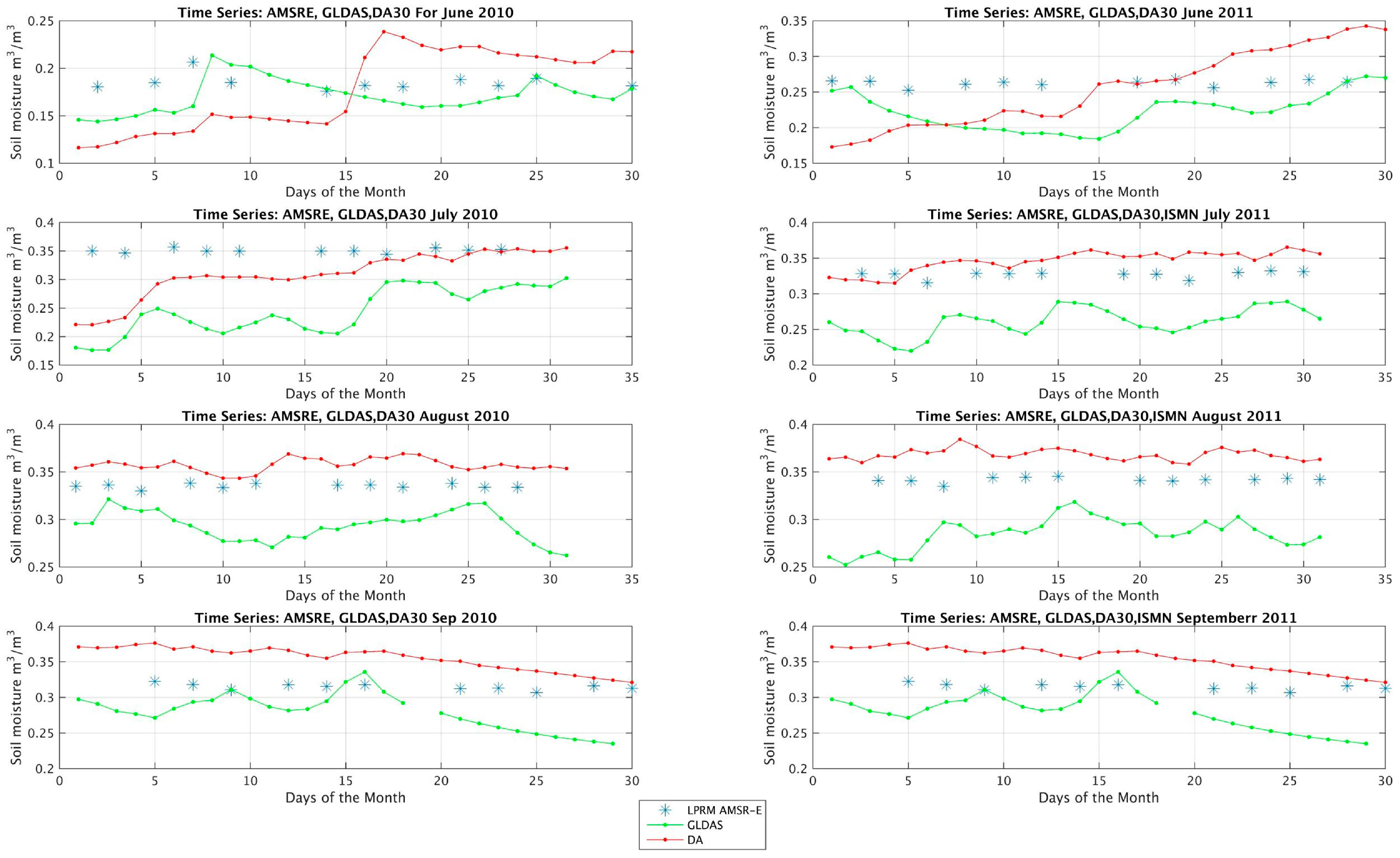
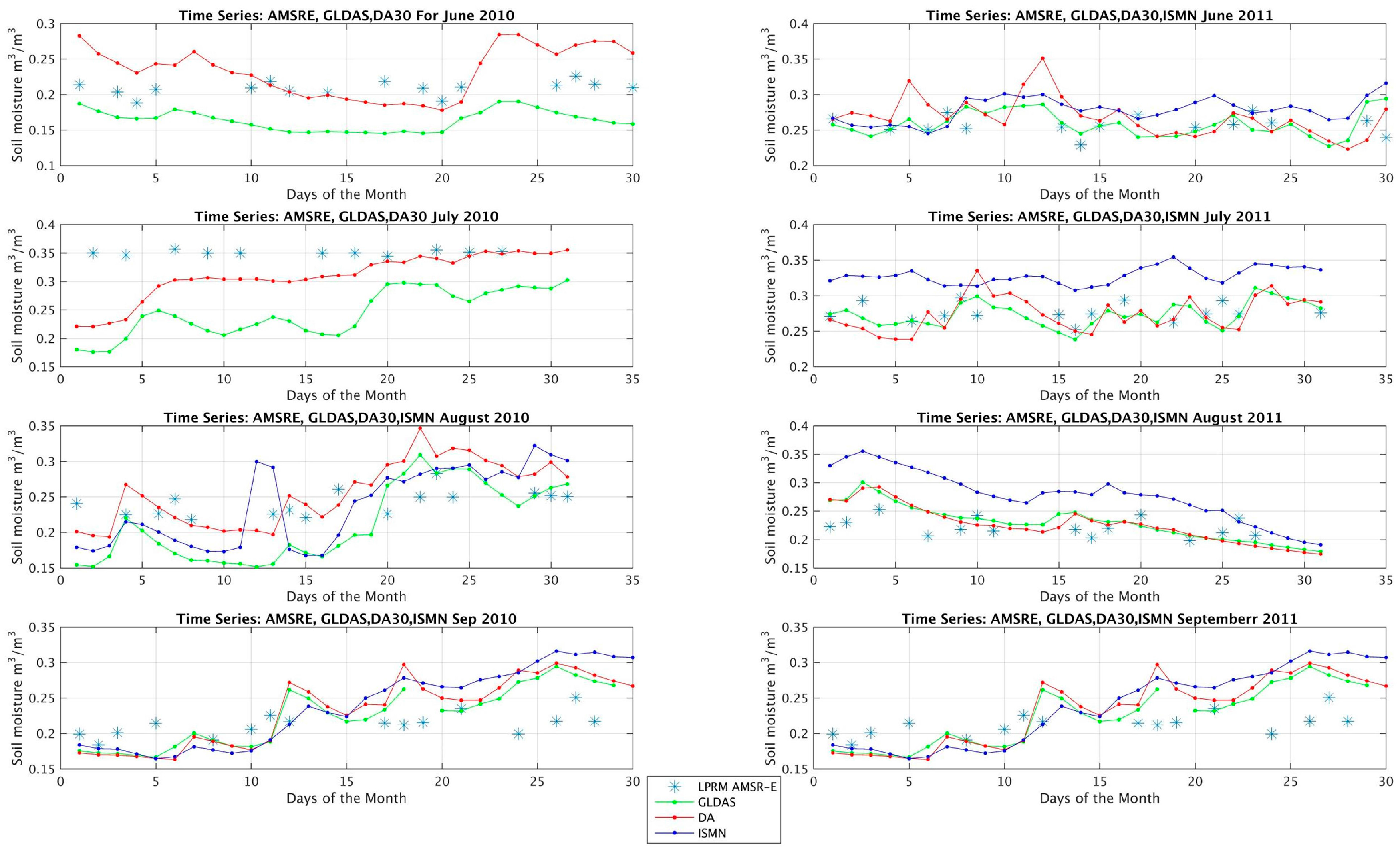
- The monthly mean results for JJAS months from data assimilation were compared with the GLDAS soil moisture data and LPRM AMSR-E soil moisture. Two spatial domains within study region were studied using daily mean time series plots. Domain 1 was over central India, while domain 2 was over the Central Tibetan Plateau (CTP).In this stage, the results over the CTP were also compared with the ground soil moisture observations from ISMN data.
- (c)
- The land surface variables from the data assimilation were utilized to simulate the TOA brightness temperature at 10.7 GHz and at an incidence angle of 55°, which were compared with the actual AMSR-E Tb.
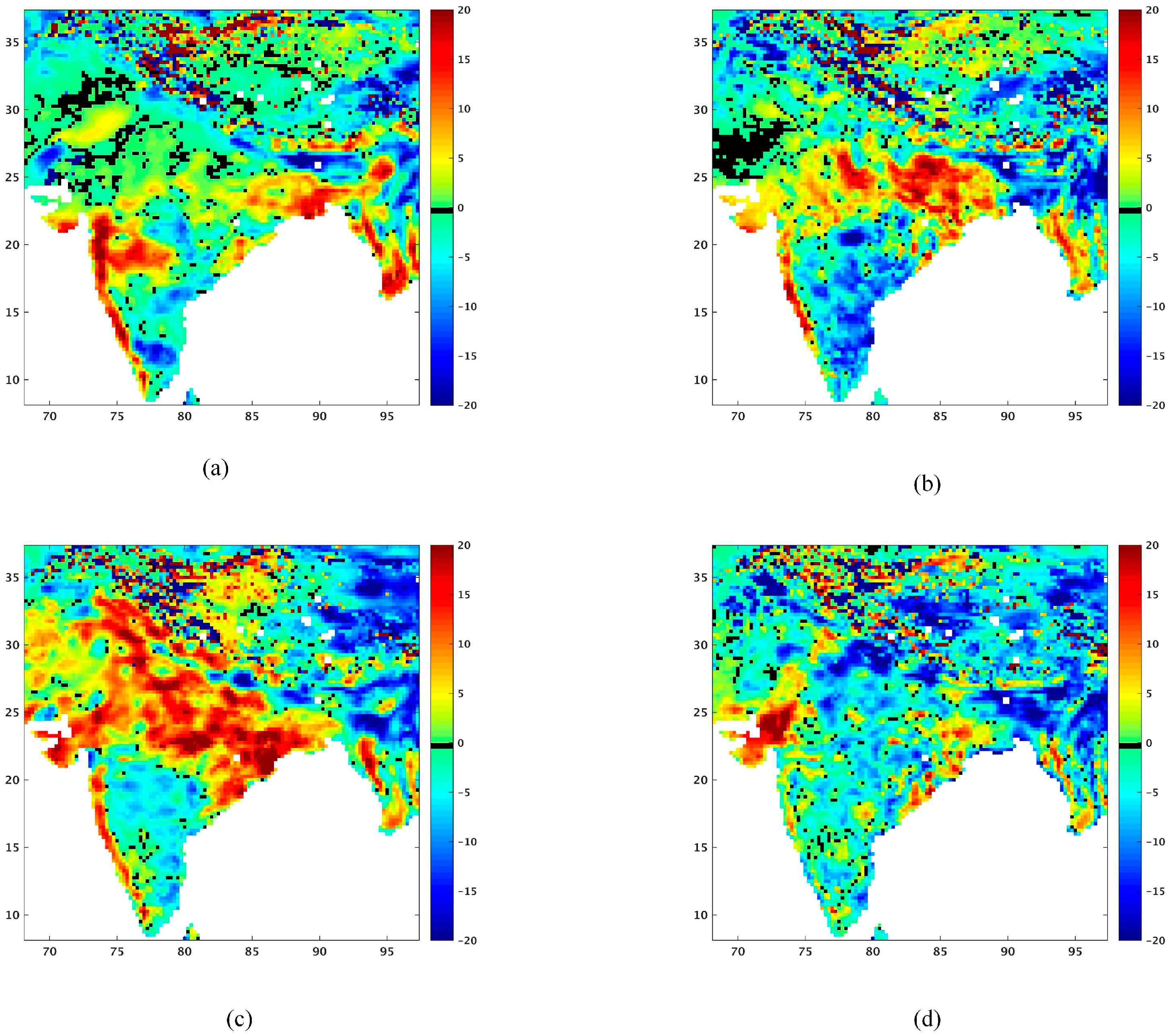
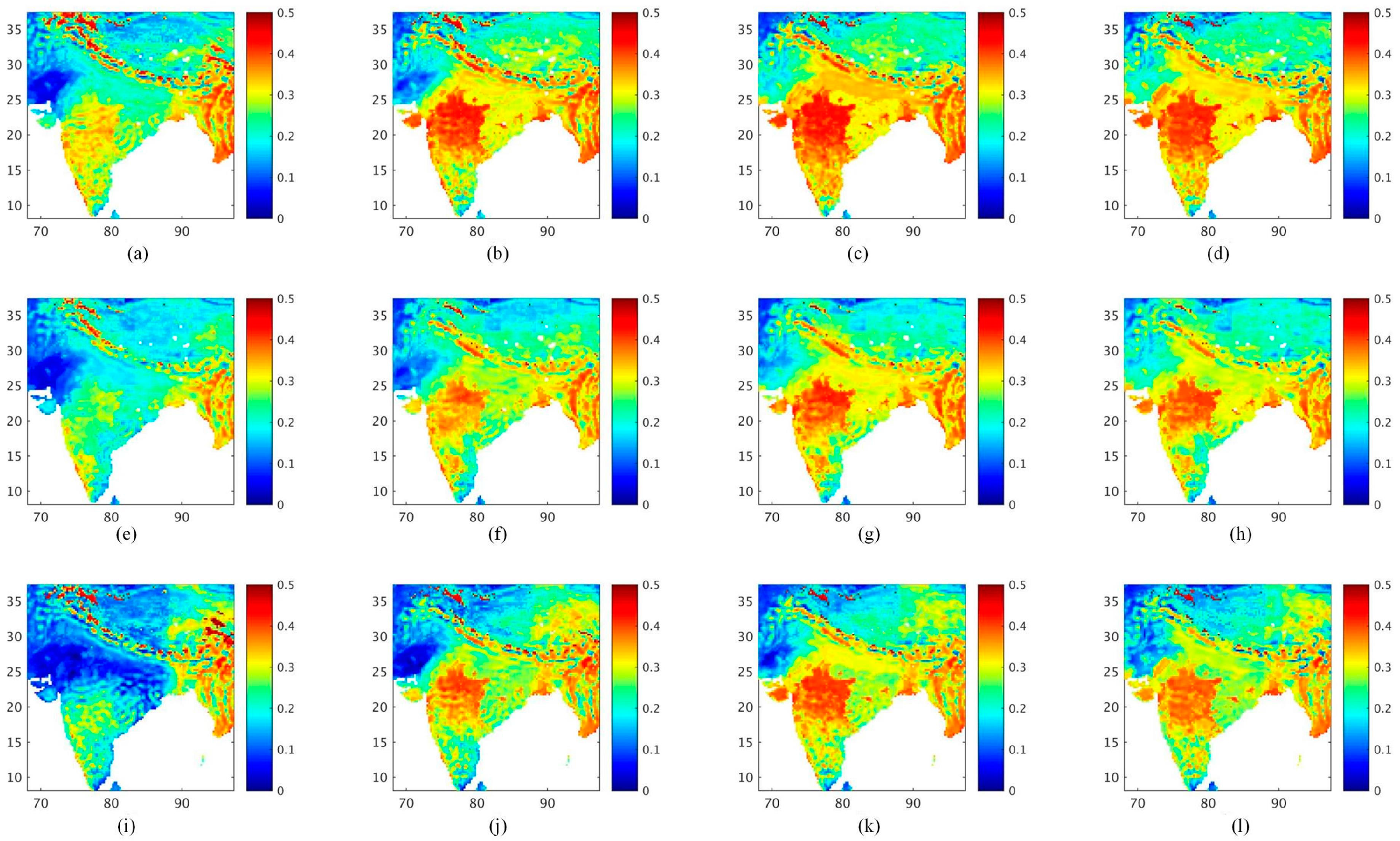
3.2. Comparing Simulated Soil Moisture with LPRM AMSR-E soil Moisture
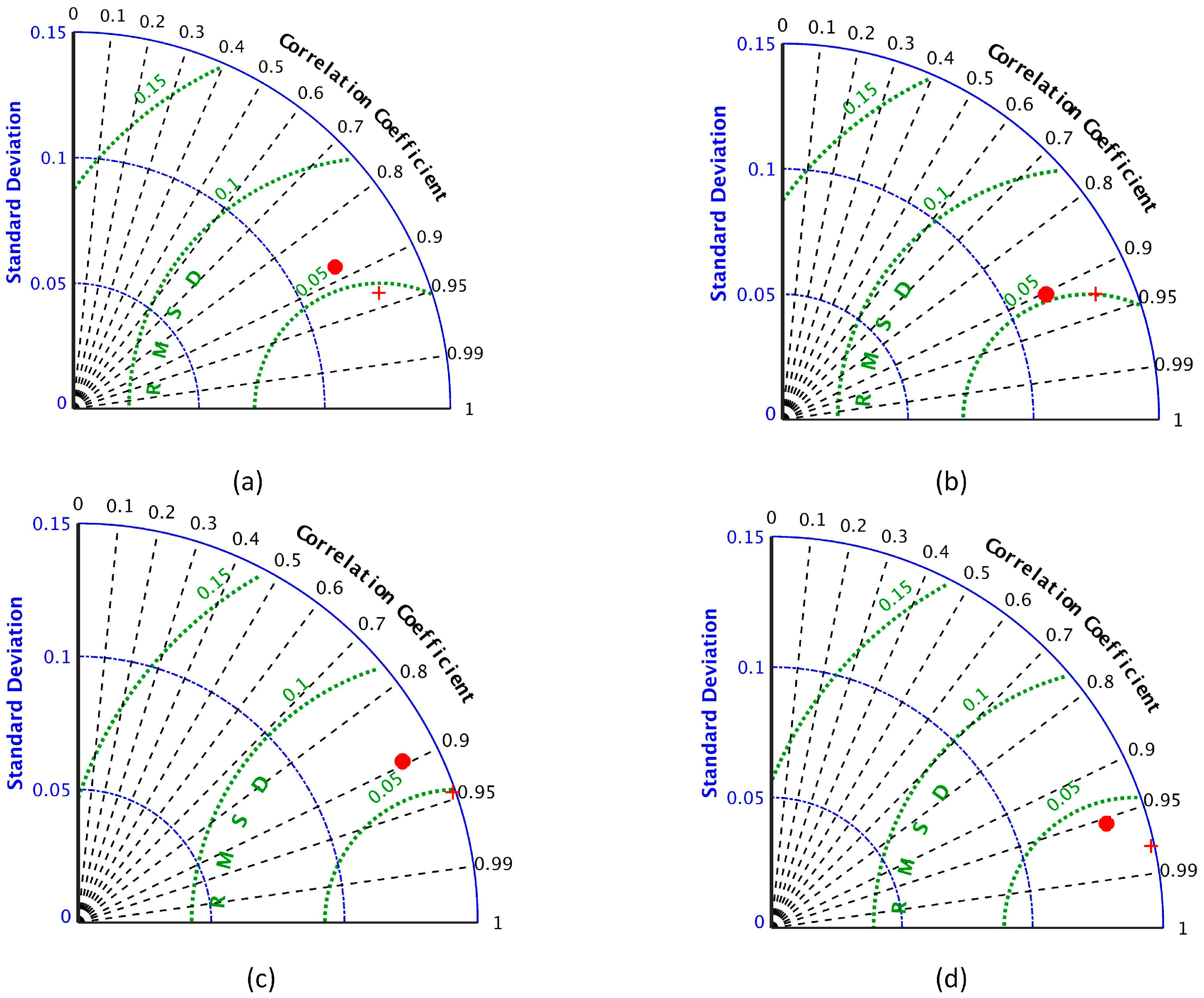
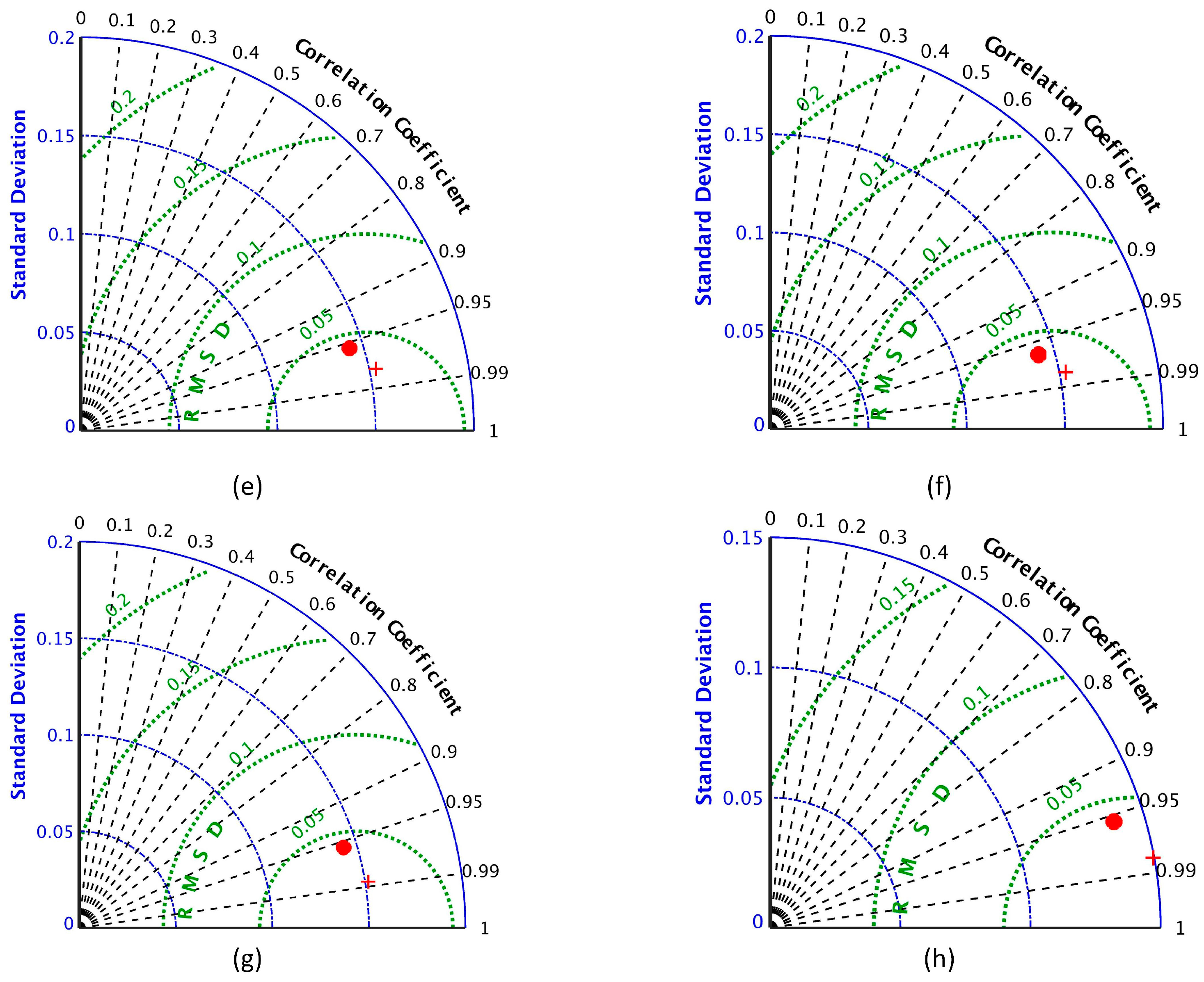
3.3. Statistical comparison between Assimilated, GLDAS and LPRM Soil Moisture
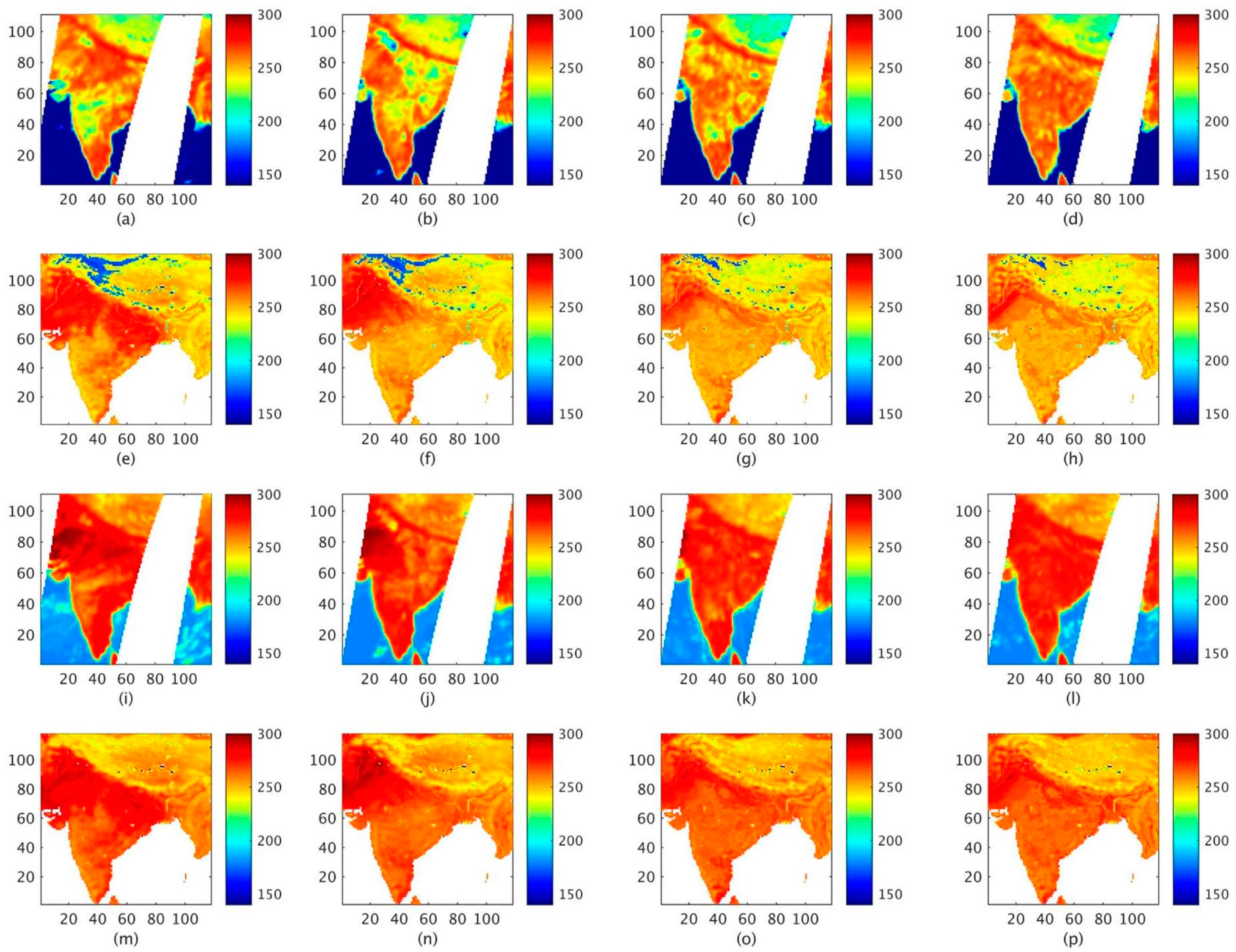
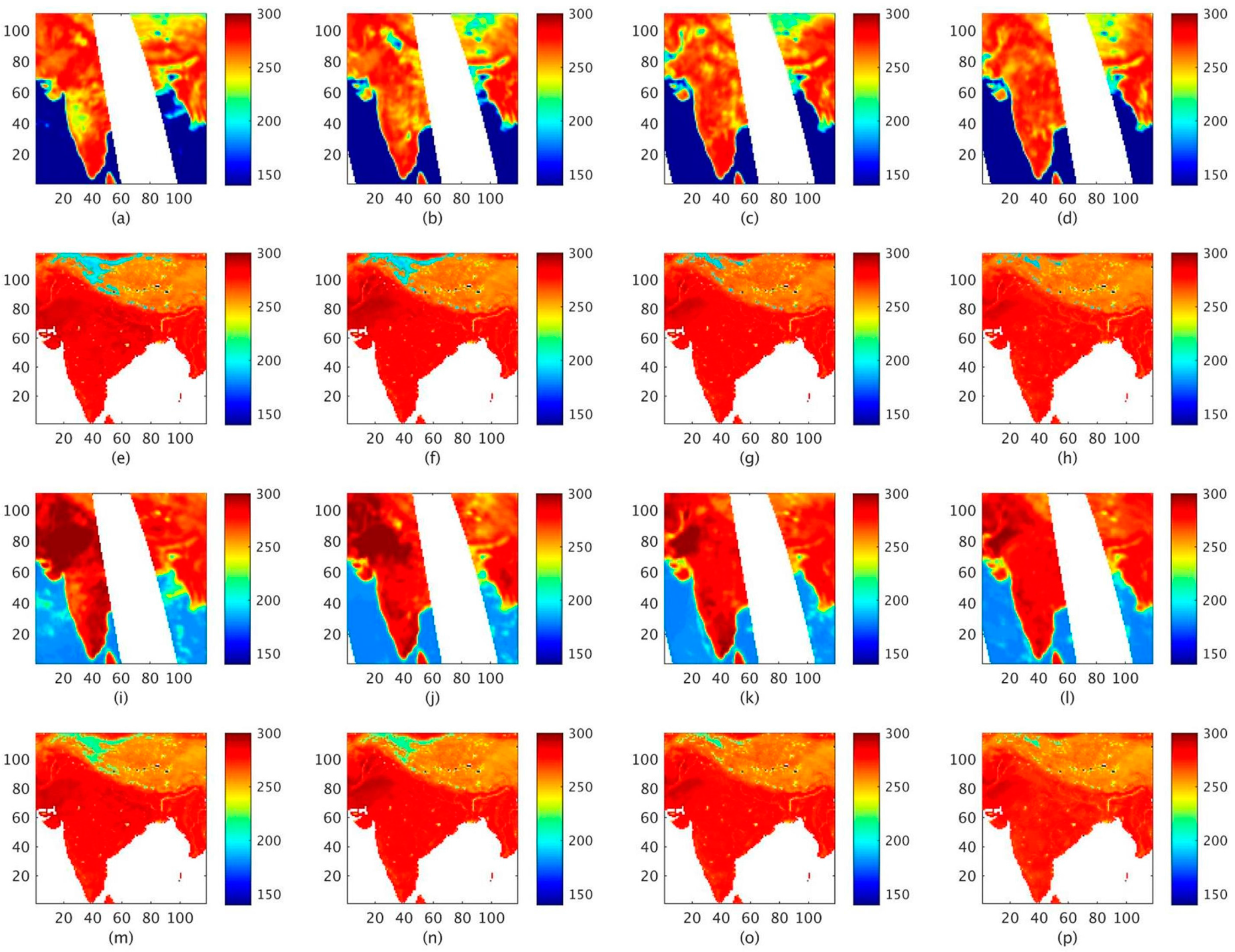
3.4. Brightness Temperature Simulation Experiment
4. Results
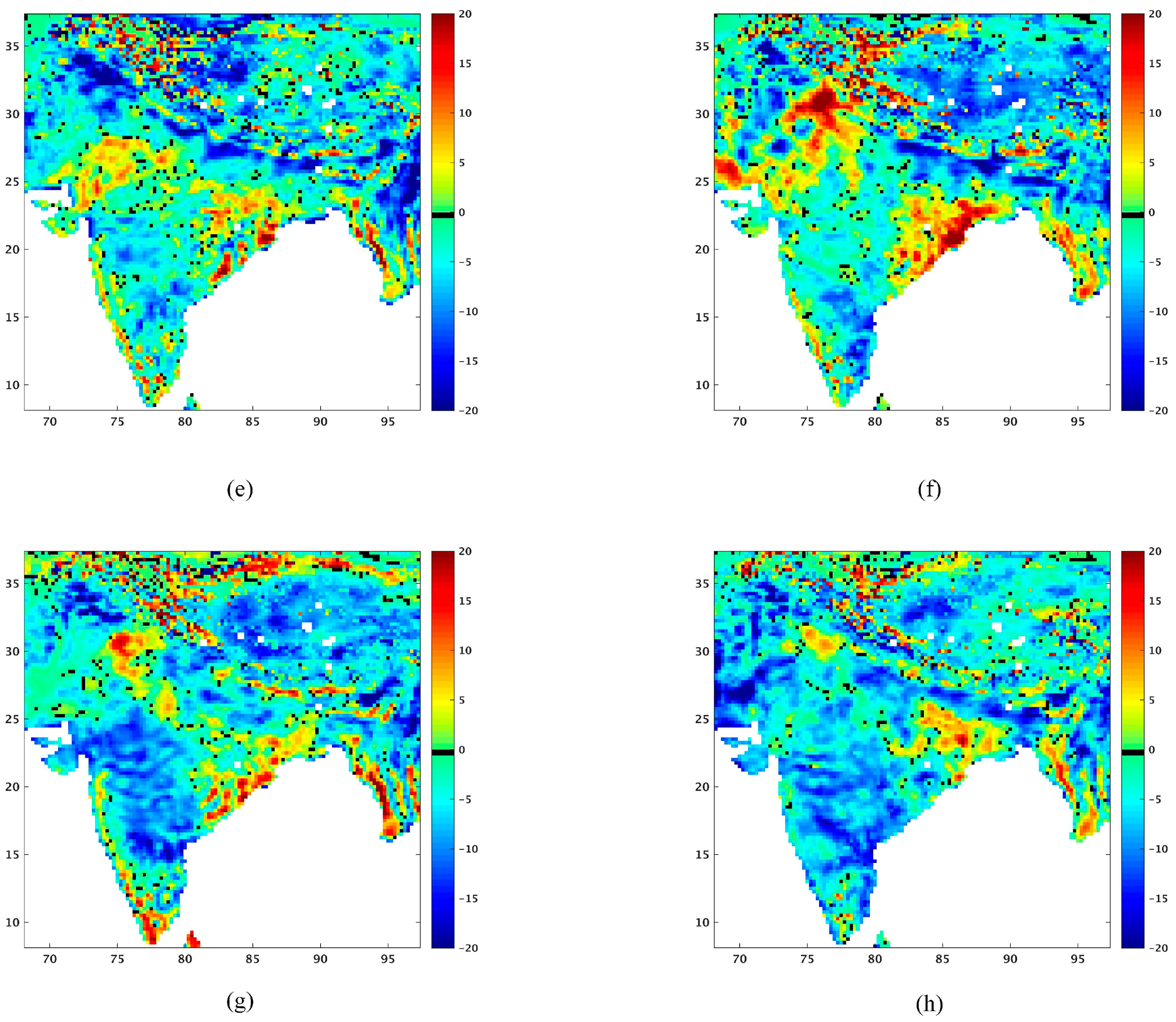
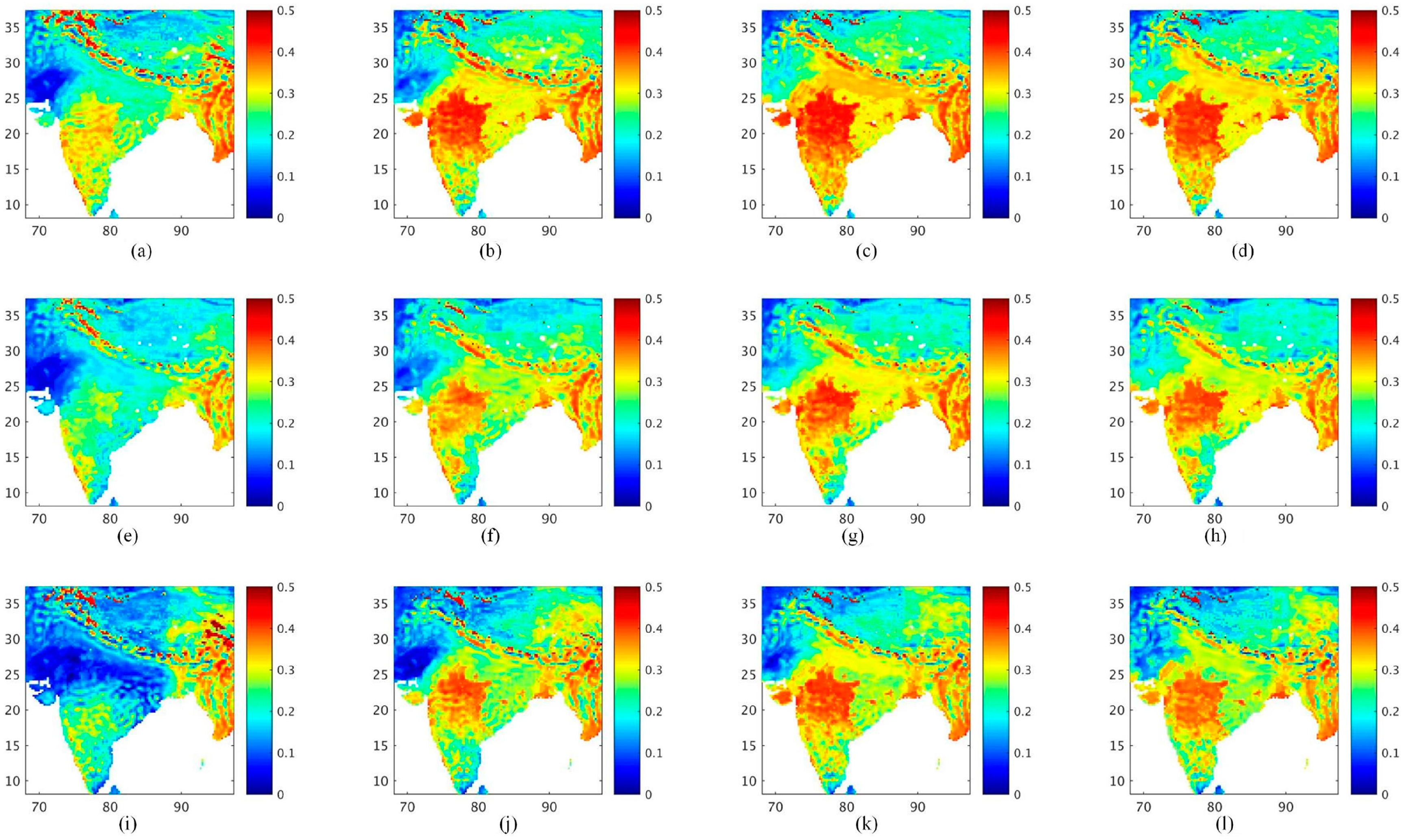
4.1. Evaluation of Simulated Soil Moisture
4.1.1. Time series plot for Domain 1 (Central India)
4.1.2. Time series plots for Domain 2 (CTP)
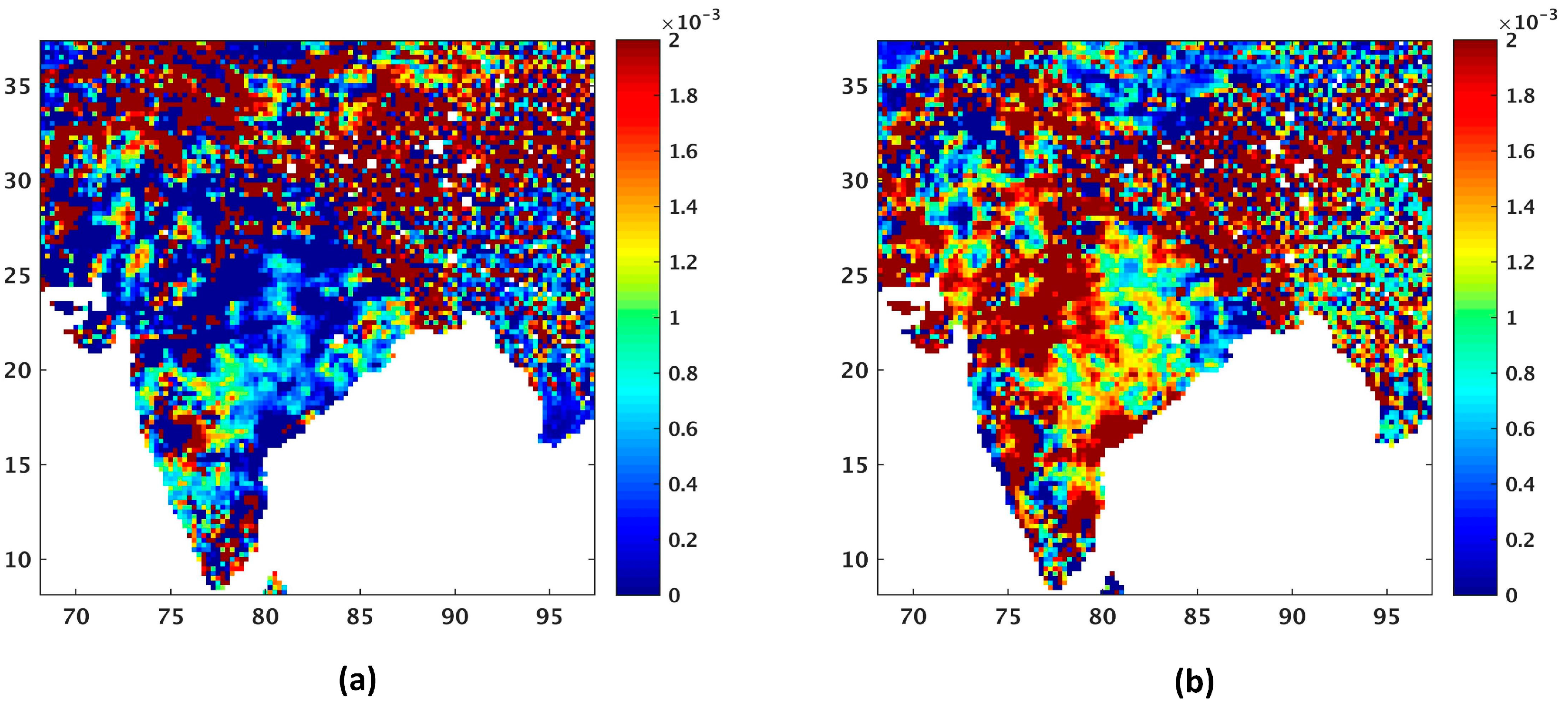
4.1.3. Error Estimation using Triple Collocation
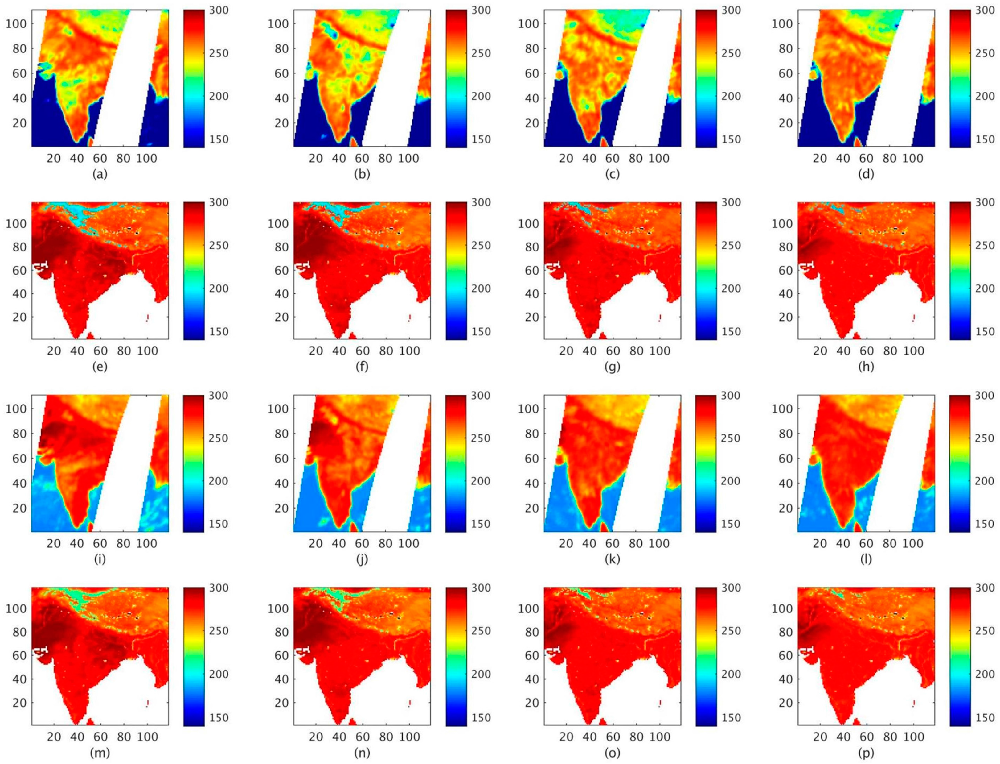
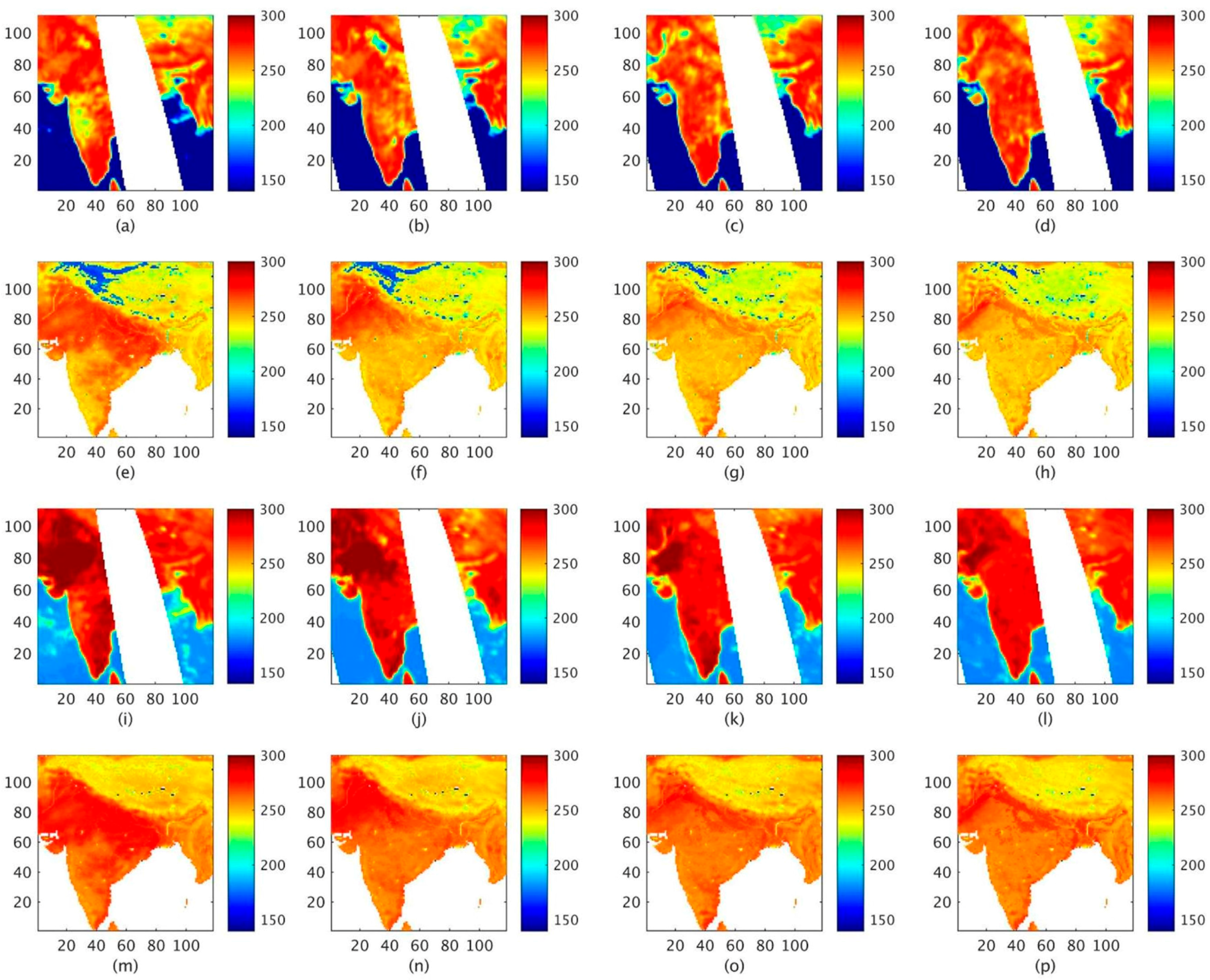
4.2. Comparisonbetween CMEM simulated and LPRM AMSR-ETB
5. Discussions
6. Summary and Conclusions
Acknowledgments
Author Contributions
Conflicts of Interest
References
- Kumar, S.V.; Harrison, K.W.; Peters-Lidard, C.D.; Santanello, J.A., Jr.; Kirschbaum, D. Assessing the impact of L-band observations on drought and flood risk estimation: a decision-theoretic approach in an OSSE environment. J. Hydrometeorol. 2014. [Google Scholar] [CrossRef]
- Koster, R.D.; Suarez, M.J.; Liu, P.; Jambor, U.; Berg, A.; Kistler, M.; Reichle, R.; Rodell, M.; Famiglietti, J. Realistic initialization of land surface states: Impacts on subseasonal Forecast skill. J. Hydrometeorol. 2004. [Google Scholar] [CrossRef]
- Chen, F.; Mitchell, K.; Schaake, J.; Xue, Y.; Pan, H.; Koren, V.; Duan, Q.Y.; Ek, M.; Betts, A. Modeling of land surface evaporation by four schemes and comparison with FIFE observations. J. Geophys. Res. 1996. [Google Scholar] [CrossRef]
- Koren, V.; Schaake, J.; Mitchell, K.; Duan, Q.Y.; Chen, F.; Baker, J.M. A parameterization of snowpack and frozen ground intended for NCEP weather and climate models. J. Geophys. Res. 1999. [Google Scholar] [CrossRef]
- Dai, Y.; Zeng, X.; Dickinson, R.E.; Baker, I. The common land model. Bull. Am. Meteorol. Soc. 2003, 84, 1013–1023. [Google Scholar] [CrossRef]
- Xu, L.; Dennis, P.L.; Eric, F.W.; Burges, J.S. A simple hydrological based model of land surface water and energy fluxes for general circulation models. J. Geophys. Res. 1994. [Google Scholar] [CrossRef]
- Randal, D.K.; Max, J.S. Energy and Water Balance Calculations in the Mosaic LSM; National Aeronautics and Space Administration: Greenbelt, ML, USA, 1996. [Google Scholar]
- Rolf, H.R.; McLaughlin, D.B.; Entekhabi, D. Hydrological data assimilation with the ensemble Kalman Filter. J. Hydrometeorol. 2002. [Google Scholar] [CrossRef]
- Daley, R. Atmospheric Data Analysis; Cambridge University Press: Cambridge, UK, 1991. [Google Scholar]
- Bennett, A.F. Inverse Methods in Physical Oceanography; Cambridge University Press: Cambridge, UK, 1992. [Google Scholar]
- Dennis, M. An integrated approach to hydrological data assimilation: Interpolation, smoothing, and filtering. Adv. Water Resour. 2002. [Google Scholar] [CrossRef]
- Walker, J.P.; Houser, P.R. A methodology for initializing soil moisture in a global climate model: Assimilation of near-surface soil moisture observations. J. Geophys. Res. 2001, 106, 11761–11774. [Google Scholar] [CrossRef]
- Walker, J.P.; Garry, W.R.; Kalma, J.D. Three-dimensional soil moisture profile retrieval by assimilation of near-surface measurements: Simplified Kalman filter covariance forecasting and field application. Water Resour. Res. 2002. [Google Scholar] [CrossRef]
- Che, T.; Li, X.; Jin, R.; Huang, C. Assimilating passive microwave remote sensing data into a land surface model to improve the estimation of snow depth. Remote Sens. Environ. 2014. [Google Scholar] [CrossRef]
- Dunne, S.; Entekhabi, D. An ensemble-based reanalysis approach to land data assimilation. Water Resour. Res. 2005. [Google Scholar] [CrossRef]
- Yang, K.; Zhu, L.; Chen, Y.; Zhao, L.; Qin, J.; Lu, H.; Tang, W.; Han, M.; Ding, B.; Fang, N. Land surface model calibration through microwave data assimilation for improving soil moisture simulations. J. Hydrol. 2015. [Google Scholar] [CrossRef]
- Rodell, M.; Houser, R.P.; Jambor, A.U.E.; Gottschalck, J. The global land data assimilation system. Bull. Am. Meteorol. Soc. 2004, 3, 381–394. [Google Scholar] [CrossRef]
- Njoku, E.G.; Jackson, T.J.; Lakshmi, V.; Chan, T.K.; Nghiem, S.V. Soil moisture retrieval from AMSR-E. IEEE Trans. Geosci. Remote Sens. 2003, 41, 215–227. [Google Scholar] [CrossRef]
- Li, L.; Gaiser, P.W.; Gao, B.; Bevilacqua, R.M.; Jackson, T.J.; Njoku, E.G.; Rudiger, C.; Calvet, J.; Bindlish, R. WindSat global soil moisture retrieval and validation. IEEE Trans. Geosci. Remote Sens. 2010, 48, 2224–2241. [Google Scholar] [CrossRef]
- Al-Yaari, A.; Wigneron, J.P.; Ducharne, A.; Kerr, Y.; De Rosnay, P.; De Jeu, R.; Govind, A.; Al Bitar, A.; Albergel, C.; Munoz-Sabater, J.; et al. Global-scale evaluation of two satellite-based passive microwave soil moisture datasets (SMOS and AMSR-E) with respect to land data assimilation system estimates. Remote Sens. Environ. 2014, 149, 181–195. [Google Scholar] [CrossRef]
- Dente, L.; Su, Z.; Wen, J. Validation of SMOS soil moisture products over the Maqu and Twente Regions. Sensors 2012, 12, 9965–9986. [Google Scholar] [CrossRef] [PubMed]
- Jackson, T.J.; Bindlish, R.; Cosh, M.H.; Zhao, T.; Starks, P.J.; Bosch, D.D.; Seyfried, M.; Moran, M.S.; Goodrich, D.C.; Kerr, Y.H.; Leroux, D. Validation of soil moisture and ocean salinity (SMOS) soil moisture over watershed networks in the U.S. IEEE Trans. Geosci. Remote Sens. 2012, 50, 1530–1543. [Google Scholar] [CrossRef]
- Sanchez, N.; Martinez-Fernandez, J.; Scaini, A.; Perez-Gutierrez, C. Validation of the SMOS L2 soil moisture data in the REMEDHUS Network (Spain). IEEE Trans. Geosci. Remote Sens. 2012, 50, 1602–1611. [Google Scholar] [CrossRef]
- Rolf, H.R. Data assimilation methods in the Earth sciences. Adv. Water Resour. 2008. [Google Scholar] [CrossRef]
- Zhan, X.; Liu, J.; Zhao, L.; Jensen, K. Soil Moisture Operational Product System (SMOPS) Algorithm Theoretical Basis Document; NOAA NESDIS STAR: Suitland, MD, USA, 2011. [Google Scholar]
- Owe, M.; de Jeu, R.; Holmes, T. Multisensor historical climatology of satellite-derived global land surface moisture. J. Geophys. Res. 2008. [Google Scholar] [CrossRef]
- Rüdiger, C.; Calvet, J.; Gruhier, C.; Holmes, T.R.H.; de Jeu, R.A.M.; Wagner, W. An intercomparison of ERS-Scat and AMSR-E soil moisture observations with model simulations over France. J. Hydrometeorol. 2009. [Google Scholar] [CrossRef]
- Derber, J.C.; Parrish, D.F.; Lord, S.J. The new global operational analysis system at the national meteorological center. Weather Forecast. 1991. [Google Scholar] [CrossRef]
- Chempeaux, J.L.; Masson, V.; Chauvin, F. ECOCLIMAP: A global database of land surface parameters at 1 km resolution. Meteorol. Appl. 2005. [Google Scholar] [CrossRef]
- Yang, K.; Qin, J.; Zhao, L.; Chen, Y.; Tang, W.; Han, M.; Chen, Z.; Lv, N.; Ding, B.; Wu, H.; Lin, C. A multi-scale soil moisture and freeze-thaw monitoring network on the third pole. Bull. Am. Meteorol. Soc. 2013. [Google Scholar] [CrossRef]
- Kumar, S.V.; Peters-Lidard, C.D.; Tian, Y.; Houser, P.R.; Geiger, J.; Olden, S.; Lighty, L.; Eastman, J.L.; Doty, B.; Dirmeyer, P.; Adams, J. Land Information system—An interoperable framework for high resolution land surface modeling. Environ. Model. Softw. 2006, 21, 1402–1415. [Google Scholar] [CrossRef]
- Peters-Lidard, C.D.; Houser, P.R.; Tian, Y.; Kumar, S.V.; Geiger, J.; Olden, S.; Lighty, L.; Doty, B.; Dirmeyer, P.; Adams, J.; Mitchell, K. High-performance Earth system modeling with NASA/GSFC’s land information system. Innov. Syst. Softw. Eng. 2007. [Google Scholar] [CrossRef]
- Mahrt, L.; Pan, H. A Two-Layer model of soil hydrology. Boundary-Layer Meteorol. 1984. [Google Scholar] [CrossRef]
- Ek, M.B.; Mitchell, K.E.; Lin, Y.; Rogers, E.; Grunmann, P.; Koren, V.; Gayno, G.; Tarpley, J.D. Implementation of Noah land surface model advances in the National Centers for Environmental Prediction operational mesoscale Eta model. J. Geophys. Res. 2003. [Google Scholar] [CrossRef]
- Mahrt, L.; Ek, M. The influence of atmospheric stability on potential evaporation. J. Clim. Appl. Meteorol. 1984. [Google Scholar] [CrossRef]
- Pan, H.L.; Mahrt, L. Interaction between soil hydrology and boundary-layer development. Boundary-Layer Meteorol. 1987. [Google Scholar] [CrossRef]
- Rodell, M.; Houser, P.R.; Berg, A.A.; Famiglietti, J.S. Evaluation of 10 methods for initializing a land surface model. J. Hydrometeorol. 2005. [Google Scholar] [CrossRef]
- Yang, Z.L.; Dickinson, R.E.; Henderson-Sellers, A.; Pitman, A.J. Preliminary study of spin-up processes in land surface models with the first stage data project for Intercomparison of Land Surface Parameterization Schemes Phase 1(a). J. Geophys. Res. 1995. [Google Scholar] [CrossRef]
- Margulis, S.A.; McLaughlin, D.; Entekhabi, D.; Dunne, S. Land data assimilation and estimation of soil moisture using measurements from the Southern Great Plains 1997 field experiment. Water Resour. Res. 2002. [Google Scholar] [CrossRef]
- Kumar, S.V.; Peters-Lidard, C.D.; Santanello, J.A.; Reichle, R.H.; Draper, C.S.; Koster, R.D.; Nearing, G.; Jasinski, M.F. Evaluating the utility of satellite soil moisture retrievals over irrigated areas and the ability of land data assimilation methods to correct for unmodeled processes. Hydrol. Earth Syst. Sci. 2015, 19, 4463–4478. [Google Scholar] [CrossRef]
- Yin, J.; Zhan, X.; Zheng, Y.; Liu, J.; Fang, L.; Hain, C.R. Enhancing Model Skill by assimilating SMOPS blended soil moisture product into Noah land surface model. J. Hydrometeorol. 2015. [Google Scholar] [CrossRef]
- Reichle, R.H.; Koster, R.D. Assessing the impact of horizontal error correlations in background fields on soil moisture estimation. J. Hydrometeorol. 2003. [Google Scholar] [CrossRef]
- Kumar, S.V.; Reichle, R.H.; Peters-Lidard, C.D.; Koster, R.D.; Zhan, X.; Crow, W.T.; Eylander, J.B.; Houser, P.R. A land surface data assimilation framework using the land information system: Description and applications. Adv. Water Resour. 2008, 31, 1419–1432. [Google Scholar] [CrossRef]
- Drusch, M.; Holmes, T.; de Rosnay, P.; Balsamo, G. Comparing ERA-40-based L-band brightness Temperature with Skylab Observations: A calibration/validation study using the community microwave emission model. J. Hydrometeorol. 2009. [Google Scholar] [CrossRef]
- Wigneron, J.P.; Kerr, Y.; Waldteufel, P.; Saleh, K.; Escorihuela, M.J.; Richaume, P.; Ferrazzoli, P.; de Rosnay, P.; Gurney, R.; Calvet, J.C.; Grant, J.P. L-band Microwave Emission of the Biosphere (L-MEB) Model: Description and calibration against experimental data sets over crop fields. Remote Sens. Environ. 2007, 107, 639–655. [Google Scholar] [CrossRef]
- de Rosnay, P.; Drusch, M.; Boone, A.; Balsamo, G.; Decharme, B.; Harris, P.; Kerr, Y.; Pellarin, T.; Polcher, J.; Wigneron, J.P. AMMA land surface model intercomparison experiment coupled to the Community Microwave Emission Model: ALMIP-MEM. J. Geophys. Res. 2009. [Google Scholar] [CrossRef]
- Jia, B.; Xie, Z. Evaluation of the community microwave emission model coupled with the community land model over East Asia. Atmos. Ocean. Sci. Lett. 2015. [Google Scholar] [CrossRef]
- Cho, E.; Choi, M.; Wagner, W. An assessment of remotely sensed surface and root zone soil moisture through active and passive sensors in northeast Asia. Remote Sens. Environ. 2015, 160, 166–179. [Google Scholar] [CrossRef]
- Pellarin, T.; Calvet, J.; Wagner, W. Evaluation of ERS scatterometer soil moisture products over a half-degree region in southwestern France. Geophys. Res. Lett. 2006. [Google Scholar] [CrossRef]
- Bi, H.; Ma, J.; Zheng, W.; Zeng, J. Comparison of soil moisture in GLDAS model simulations and in situ observations over the Tibetan Plateau. J. Geophys. Res. Atm. 2016. [Google Scholar] [CrossRef]
- Taylor, K.E. Summarizing multiple aspects of model performance in a single diagram. J. Geophys. Res. 2001. [Google Scholar] [CrossRef]
- Stoffelen, A.D. Towards the true near-surface wind speed: Error modeling and calibration using triple collocation. J. Geophys. Res. 1998, 103, 7755–7766. [Google Scholar] [CrossRef]
- McColl, K.A.; Vogelzang, J.; Konings, A.G.; Entekhabi, D.; Piles, M.; Stoffelen, A. Extended triple collocation: Estimating errors and correlation coefficients with respect to an unknown target. Geophys. Res. Lett. 2014. [Google Scholar] [CrossRef]
- Su, C.; Ryu, D.; Crow, W.T.; Western, A.W. Beyond triple collocation: Applications to soil moisture monitoring. J. Geophys. Res. Atmos. 2014. [Google Scholar] [CrossRef]
- Tian, X.; Xie, Z.; Dai, A.; Jia, B.; Shi, C. A microwave land data assimilation system: Scheme and preliminary evaluation over China. J. Geophys. Res. 2010. [Google Scholar] [CrossRef]
- Jia, B.; Tian, X.; Xie, Z.; Liu, J.; Shi, C. Assimilation of microwave brightness temperature in land data assimilation system with multi-observation operators. J. Geophys. Res. Atmos. 2013. [Google Scholar] [CrossRef]
- de Lannoy, G.J.M.; Reichle, R.H.; Pauwels, V.R.N. Global calibration of the GEOS-5 L-band microwave radiative transfer model over nonfrozen land using SMOS observations. J. Hydrometeorol. 2013. [Google Scholar] [CrossRef]
- Brocca, L.; Hasenauer, S.; Lacava, T.; Melone, F.; Moramarco, T.; Wagner, W.; Dorigo, W.; Matgen, P.; Martínez-Fernández, J.; Llorens, P.; Latron, J. Soil Moisture estimation through ASCAT and AMSR-E sensors: An intercomparison and validation study across Europe. Remote Sens. Environ. 2011, 115, 3390–3408. [Google Scholar] [CrossRef]
- Yang, K.; Chen, Y.Y.; Qin, J. Some pratical notes on the land surface modeling in the Tibetan Plateau. Hydrol. Earth Syst. Sci. 2009, 13, 687–701. [Google Scholar] [CrossRef]
- Chen, Y.; Yang, K.; Qin, J.; Zhao, L.; Tang, W.; Han, M. Evaluation of AMSR-E retrievals and GLDAS simulations against observations of a soil moisture network on the central Tibetan Plateau. J. Geophys. Res. Atmos. 2013. [Google Scholar] [CrossRef]
- Reynolds, C.A.; Jackson, T.J.; Rawls, W.J. Estimating soil water-holding capacities by linking the Food And Agriculture Organization soil map of the world with global pedon database and continuous pedotransfer functions. Water Resour. Res. 2000. [Google Scholar] [CrossRef]
- Albergel, C.; Calvet, J.C.; De Rosnay, P.; Balsamo, G.; Wagner, W.; Hasenauer, S.; Naeimi, V.; Martin, E.; Bazile, E.; Bouyssel, F.; Mahfouf, J.F. Cross-evaluation of modelled and remotely sensed surface soil moisture with in situ data in southwestern France. Hydrol. Earth Syst. Sci. 2010, 14, 2177–2191. [Google Scholar] [CrossRef]
- Wei, S.; Dai, Y.; Liu, B.; Zhu, A.; Duan, Q.; Wu, L.; Ji, D.; Ye, A.; Yuan, H.; Zhang, Q.; Chen, D. A China data set of soil properties for land surface modeling. J. Adv. Model. Earth Syst. 2013. [Google Scholar] [CrossRef]


| Variable | Spatial Resolution | Temporal Resolution | Source |
|---|---|---|---|
| Forcing Data | |||
| Near surface air temperature | 0.47° × 0.47° | 3 Hourly | GDAS |
| Near surface specific humidity | |||
| Total incident shortwave radiation | |||
| Incident Longwave Radiation | |||
| Eastward wind | |||
| Northward wind | |||
| Surface pressure | |||
| Rainfall rate | |||
| Convective rainfall rate | |||
| LSM Parameters | |||
| Landcover | 0.01 × 0.01 | - | AVHRR/UMD |
| Soil Texture | 0.25 × 0.25 | - | FAO |
| Soil Fraction (clay, sand, silt) | 0.25 × 0.25 | - | FAO |
| Slope type | 0.01 × 0.01 | - | NCEP_LIS |
| Elevation Data | - | - | SRTM |
| Albedo | 0.01 × 0.01 | Monthly | NCEP_LIS |
| Greenness fraction | 0.01 × 0.01 | - | NCEP_LIS |
| RTM Parameters | |||
| Soil fraction | 0.25 × 0.25 | - | Ecoclimap/FAO |
| Geopotential | 0.25 × 0.25 | - | NCEP |
| Vegetation fraction | 0.25 × 0.25 | - | Ecoclimap |
| Vegetation Type | 0.25 × 0.25 | - | Ecoclimap |
| Variable | Perturbation Type | Standard Deviation | Cross Correlation | ||||
|---|---|---|---|---|---|---|---|
| P | SW | LW | |||||
| Forcing Perturbation | Precipitation (P) | Multiplicative | 0.5 (mm) | 1.0 | −0.8 | 0.5 | |
| Downward Shortwave (SW) | Multiplicative | 0.3 (W·m−2) | −0.8 | 1.0 | −0.5 | ||
| Downward Longwave (LW) | Additive | 50 (W·m−2) | 0.5 | −0.5 | 1.0 | ||
| SM1 | SM2 | SM3 | SM4 | ||||
| State Variable Perturbation | SM Layer 1 | Additive | 6.00 × 10⁻³ m3·m−3 | 1.0 | 0.6 | 0.4 | 0.2 |
| SM Layer 2 | Additive | 1.10 × 10⁻⁴ m3·m−3 | 0.6 | 1.0 | 0.6 | 0.4 | |
| SM Layer 3 | Additive | 6.00 × 10⁻⁵ m3·m−3 | 0.4 | 0.6 | 1.0 | 0.6 | |
| SM Layer 4 | Additive | 4.00 × 10⁻⁵ m3·m−3 | 0.2 | 0.4 | 0.6 | 1.0 | |
| Module | Variable | Parameterization | |
|---|---|---|---|
| Scheme One | Scheme Two | ||
| Soil | Soil dielectric constant | Wang | Wang |
| Soil effective temperature | Choudhury | Choudhury | |
| Smooth emissivity | Fresnel | Fresnel | |
| Soil roughness | Choudhury | Wegmueller | |
| Vegetation | Vegetation optical depth | Kirdyashev | Wigneron |
| Atmosphere | Atmospheric optical depth | Pellarin | Pellarin |
| Snow | Snow reflectivity | Pulliainen | Pulliainen |
| LPRM AMSR-E | DA | GLDAS | ||
|---|---|---|---|---|
| Correlation(r) | 10 June | 1 | 0.9349 | 0.8789 |
| 11 June | 1 | 0.9277 | 0.9029 | |
| 10 July | 1 | 0.9444 | 0.8952 | |
| 11 July | 1 | 0.9773 | 0.9546 | |
| 10 August | 1 | 0.9786 | 0.9501 | |
| 11 August | 1 | 0.9819 | 0.9637 | |
| 10 September | 1 | 0.9874 | 0.9567 | |
| 11 September | 1 | 0.9837 | 0.9555 | |
| RMSD | 10 June | 0 | 0.0462 | 0.0593 |
| 11 June | 0 | 0.0502 | 0.0528 | |
| 10 July | 0 | 0.0490 | 0.0641 | |
| 11 July | 0 | 0.0321 | 0.0415 | |
| 10 August | 0 | 0.0320 | 0.0453 | |
| 11 August | 0 | 0.0298 | 0.0384 | |
| 10 September | 0 | 0.0248 | 0.0422 | |
| 11 September | 0 | 0.0279 | 0.0415 | |
| Standard Deviation | 10 June | 0.1221 | 0.1300 | 0.1185 |
| 11 June | 0.1219 | 0.1344 | 0.1162 | |
| 10 July | 0.1426 | 0.1489 | 0.1360 | |
| 11 July | 0.1391 | 0.1487 | 0.1343 | |
| 10 August | 0.1451 | 0.1534 | 0.1360 | |
| 11 August | 0.1434 | 0.1531 | 0.1417 | |
| 10 September | 0.1435 | 0.1516 | 0.1430 | |
| 11 September | 0.1398 | 0.1496 | 0.1382 | |
© 2016 by the authors; licensee MDPI, Basel, Switzerland. This article is an open access article distributed under the terms and conditions of the Creative Commons Attribution (CC-BY) license (http://creativecommons.org/licenses/by/4.0/).
Share and Cite
Nair, A.S.; Indu, J. Enhancing Noah Land Surface Model Prediction Skill over Indian Subcontinent by Assimilating SMOPS Blended Soil Moisture. Remote Sens. 2016, 8, 976. https://doi.org/10.3390/rs8120976
Nair AS, Indu J. Enhancing Noah Land Surface Model Prediction Skill over Indian Subcontinent by Assimilating SMOPS Blended Soil Moisture. Remote Sensing. 2016; 8(12):976. https://doi.org/10.3390/rs8120976
Chicago/Turabian StyleNair, Akhilesh S., and J. Indu. 2016. "Enhancing Noah Land Surface Model Prediction Skill over Indian Subcontinent by Assimilating SMOPS Blended Soil Moisture" Remote Sensing 8, no. 12: 976. https://doi.org/10.3390/rs8120976
APA StyleNair, A. S., & Indu, J. (2016). Enhancing Noah Land Surface Model Prediction Skill over Indian Subcontinent by Assimilating SMOPS Blended Soil Moisture. Remote Sensing, 8(12), 976. https://doi.org/10.3390/rs8120976