Article

Mapping Arctic Tundra Vegetation Communities Using Field Spectroscopy and Multispectral Satellite Data in North Alaska, USA

1
Department of Animal and Plant Sciences, University of Sheffield, Western Bank, Sheffield S10 2TN, UK
2
Department of Biology, San Diego State University, 5500 Campanile Drive San Diego, CA 92182, USA
3
Department of Innovation, Environmental and Energy Sciences, Utrecht University, Utrecht 3512 JE, The Netherlands
4
Numerical Terradynamic Simulation Group, ISB 428, 32 Campus Drive, The University of Montana, Missoula, MT 59812, USA
5
Department of Environment, Earth and Ecosystems, The Open University, Walton Hall, Milton Keynes MK7 6AA, UK
*
Author to whom correspondence should be addressed.
Remote Sens. 2016, 8(12), 978; https://doi.org/10.3390/rs8120978
Submission received: 22 September 2016 / Revised: 28 October 2016 / Accepted: 16 November 2016 / Published: 26 November 2016

Abstract

:
The Arctic is currently undergoing intense changes in climate; vegetation composition and productivity are expected to respond to such changes. To understand the impacts of climate change on the function of Arctic tundra ecosystems within the global carbon cycle, it is crucial to improve the understanding of vegetation distribution and heterogeneity at multiple scales. Information detailing the fine-scale spatial distribution of tundra communities provided by high resolution vegetation mapping, is needed to understand the relative contributions of and relationships between single vegetation community measurements of greenhouse gas fluxes (e.g., ~1 m chamber flux) and those encompassing multiple vegetation communities (e.g., ~300 m eddy covariance measurements). The objectives of this study were: (1) to determine whether dominant Arctic tundra vegetation communities found in different locations are spectrally distinct and distinguishable using field spectroscopy methods; and (2) to test which combination of raw reflectance and vegetation indices retrieved from field and satellite data resulted in accurate vegetation maps and whether these were transferable across locations to develop a systematic method to map dominant vegetation communities within larger eddy covariance tower footprints distributed along a 300 km transect in northern Alaska. We showed vegetation community separability primarily in the 450–510 nm, 630–690 nm and 705–745 nm regions of the spectrum with the field spectroscopy data. This is line with the different traits of these arctic tundra communities, with the drier, often non-vascular plant dominated communities having much higher reflectance in the 450–510 nm and 630–690 nm regions due to the lack of photosynthetic material, whereas the low reflectance values of the vascular plant dominated communities highlight the strong light absorption found here. High classification accuracies of 92% to 96% were achieved using linear discriminant analysis with raw and rescaled spectroscopy reflectance data and derived vegetation indices. However, lower classification accuracies (~70%) resulted when using the coarser 2.0 m WorldView-2 data inputs. The results from this study suggest that tundra vegetation communities are separable using plot-level spectroscopy with hand-held sensors. These results also show that tundra vegetation mapping can be scaled from the plot level (<1 m) to patch level (<500 m) using spectroscopy data rescaled to match the wavebands of the multispectral satellite remote sensing. We find that developing a consistent method for classification of vegetation communities across the flux tower sites is a challenging process, given the spatial variability in vegetation communities and the need for detailed vegetation survey data for training and validating classification algorithms. This study highlights the benefits of using fine-scale field spectroscopy measurements to obtain tundra vegetation classifications for landscape analyses and use in carbon flux scaling studies. Improved understanding of tundra vegetation distributions will also provide necessary insight into the ecological processes driving plant community assemblages in Arctic environments.

Graphical Abstract

1. Introduction

The Arctic is currently undergoing dramatic changes in climate [1,2,3]. As such, changes in vegetation composition and productivity are predicted to occur due to a lengthening of the growing season [4,5,6], increases in air and soil temperature and active layer depth [7,8], increased shrub cover [9,10], and acceleration of below ground microbial activity and nutrient cycling [3,11,12]. These changes influence the terrestrial carbon cycle and thus alter the relationship between arctic ecosystems and global climate. For example, an increasing growing season length can enhance carbon uptake through photosynthesis and thereby reduce atmospheric carbon dioxide (CO2) concentrations [13]. Conversely, increasing temperatures may heighten methane (CH4) and CO2 release from thawing permafrost, enhancing plant-mediated transport of CH4 [14,15] and contributing to rising levels of greenhouse gases in the atmosphere.
Carbon cycle models used to inform global climate predictions typically run at a ~1 km to 0.5° grid cell resolution, yet ecosystem carbon fluxes are most frequently measured at the plot scale (~1 m). Many of these models assume uniform vegetation composition within a cell footprint, yet in reality Arctic landscapes have high spatial heterogeneity [16]. A better understanding of the role of vegetation community composition on greenhouse gas exchange is needed to guide scaling from plot levels to coarser resolution footprints [17,18,19]. For example, Shaver et al. [20] note that changes in vegetation community composition could lead to higher ecosystem productivity, alongside increased long-term sequestration of carbon [1]. Furthermore, Ström et al. [21] note that a high proportion of carbon assimilated through photosynthesis is allocated belowground in Arctic environments, which can be impacted by different vegetation community composition. Climate warming and a lengthening growing season length may reduce cold temperature constraints on stored belowground carbon, substantially increasing ecosystem CO2 respiration or loss as CH4 [22]. Vegetation can be important in regulating CH4 emissions as plants provide labile substrates for methanogenic production. Tundra plants have structures, such as aerenchyma, which may also provide conduits for transport of CH4 from the soil to the atmosphere [14]. Although the distribution of Arctic tundra vegetation is relatively well established at coarser scales (e.g., 1:7,500,000) and documented in databases such as the Circumpolar Arctic Vegetation Map ((CAVM team, 2003; [23]) and others [24,25], knowledge of local tundra community distributions remains ambiguous at many locations. Understanding the fine-scale spatial distribution of tundra communities, combined with improved high resolution vegetation mapping, is needed to understand relative contributions of and relationships between single vegetation community measurements of greenhouse gas fluxes (e.g., ~1 m chamber flux measurements; [15]) and those encompassing multiple vegetation communities (e.g., ~100 m eddy covariance measurements; [26]).
Remote sensing allows for the assessment of vegetation across the Arctic at a variety of spatial and temporal scales under a rapidly changing climate. Moderate resolution satellite-based multispectral sensors such as the 1 km resolution Advanced Very High Resolution Radiometer (AVHRR), the 250 m to 1 km Moderate Resolution Imaging Spectroradiometer (MODIS) and the 30 m Landsat series imagers observe tundra ecosystems at daily to bi-weekly repeat cycles. These remote sensing data have been used successfully to map and monitor regional vegetation change across Arctic tundra systems [27,28], including decadal increases in biomass and greenness [29,30,31]. Although coarse spatial resolution imagery (>100 m) may be suitable for determining broad-scale ecosystem distributions and regional change, it is insufficient to capture the high spatial heterogeneity occurring across many Arctic tundra landscapes [16,32,33]. High resolution satellite data (<5 m) such as WorldView-2 may be able to capture this spatial heterogeneity, as tundra vegetation communities low stature may make it difficult to identify and quantify using coarser products [19]. However, there can be a trade-off between fine and coarser spatial resolution satellite data through temporal sampling frequency. Satellite data are often collected bi-weekly to monthly in comparison to daily repeat cycles using moderate resolution (e.g., MODIS) products. Finally, hyperspectral data have also been used successfully to map tundra vegetation, and has worked across different geographies [28,34,35,36,37], but it is only available through hand held or airborne sensors.
In complement to satellite remote sensing data, field spectroscopy provides a useful tool to characterize and map vegetation communities [29,38,39], species composition [40,41], biophysical/ecological properties [3], and plant traits [42,43] from local to landscape scales. Field spectroscopy data are not widely collected and used in Arctic tundra vegetation studies [44] due to the often difficult logistics and weather related constraints for field sampling in remote high latitude environments [45]. None-the-less, recent studies using field spectroscopy report improved spectral differentiation of vegetation communities at the plot scale [28,39,46]. For example, Bratsch et al. [39] successfully used field spectroscopy to discriminate between four tussock tundra communities at Ivotuk, Alaska with overall classification accuracies of 84%–94%. Langford et al. [47] used LiDAR data in combination with multispectral satellite imagery to map plant functional types (PFTs) at the Barrow-BEO site (also featured in this paper). However, given the tundra variability across the Alaskan landscape it is important to attempt such mapping exercises to multiple sites and combining field spectral measurements with satellite data. Further, and because of the variable conditions of the Arctic, it is important that surveys are carried-out by a consistent team, and that the timings of the surveys and imagery acquisition are well matched. Through this combination, we can test to which extent field spectroscopy can be used to map Arctic tundra communities across large landscape areas.
The goal of this research is to assess whether we could successfully map tundra vegetation communities at plot and landscape scales using detailed vegetation community analysis in conjunction with field spectroscopy and multispectral remote sensing data, across a variety of tundra types. The first objective is to first determine whether dominant tundra vegetation communities found in different locations across the Arctic Coastal Plain are spectrally distinct and distinguishable using field spectroscopy methods. Secondly, to test which combination of raw reflectance and vegetation indices retrieved from field and satellite data allows accurately mapping vegetation and across locations. To test these objectives, we developed a systematic method to map dominant vegetation communities within larger (~300 m) eddy covariance tower footprints distributed along a 300 km transect in Northern Alaska. The ability to map Arctic tundra vegetation at finer spatial scales is necessary to better understand the contribution of tundra communities to the global carbon cycle and scale related dependencies of ecological processes in various plant assemblages.

2. Materials and Methods
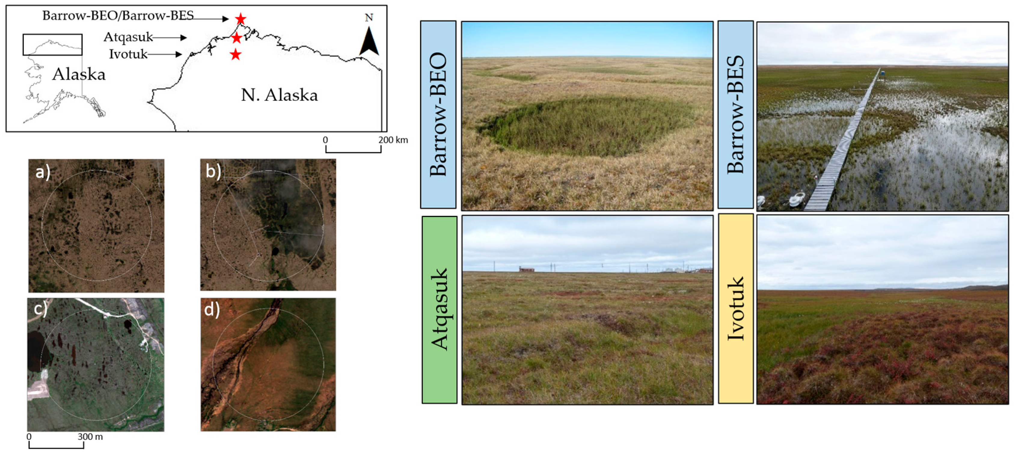
2.1. Study Area

This study was undertaken at four tower eddy covariance field sites across the North Slope of Alaska (Figure 1). Two tower sites were located near Barrow. Two additional sites were located further south towards the Brooks Range, in Atqasuk and Ivotuk.
The Barrow Environmental Observatory (Barrow-BEO; 71°16′51.61″N, 156°36′44.44″W) tower site consists of an ice-wedge polygonal tundra landscape [48], with well-developed high-, low- and flat-center polygons, whereas the other Barrow tower (hereafter Barrow-BES; 71°16′51.17″N, 156°35′47.28″W) is situated in a vegetated drained lake basin [49] approximately 300 m to the east of Barrow-BEO. Mean annual air temperature and mean summer precipitation at the Barrow sites for the 1948–2013 period was −11.3 °C and 72 mm, respectively [50]. The vegetation communities at Barrow-BEO and Barrow-BES are dominated by sedges, grasses and various mosses [23]. The third site, Atqasuk (70°28′40″N, 157°25′05″W), is located approximately 100 km south of the Barrow sites. This site includes primarily low centered, well developed polygonal tundra with well-drained high edges [24,51] and has a mean annual air temperature of −10.8 °C and a mean summer precipitation of 100 mm for the 1999–2006 period. The vegetation communities found at this site are dominated by sedges, grasses, mosses and dwarf shrubs (<40 cm) [23]. The fourth site, Ivotuk (68.49°N, 155.74°W), is located in the foothills of the Brooks Range Mountains, approximately 300 km south of Barrow. There is no substantial polygon formation located here, with the site consisting of a gentle northwest facing slope and a wet meadow on the margins of a stream. The mean annual air temperature and mean summer precipitation at this site are −8.9 °C and 210 mm respectively. The vegetation communities at Ivotuk are dominated by tussock sedge, dwarf shrubs and mosses [23]. All four tower sites are located on areas of continuous permafrost with an active layer thaw depth of approximately 37 cm [52] for Barrow-BEO/Barrow-BES, 43 cm for Atqasuk [53] and 25 cm for Ivotuk [50].

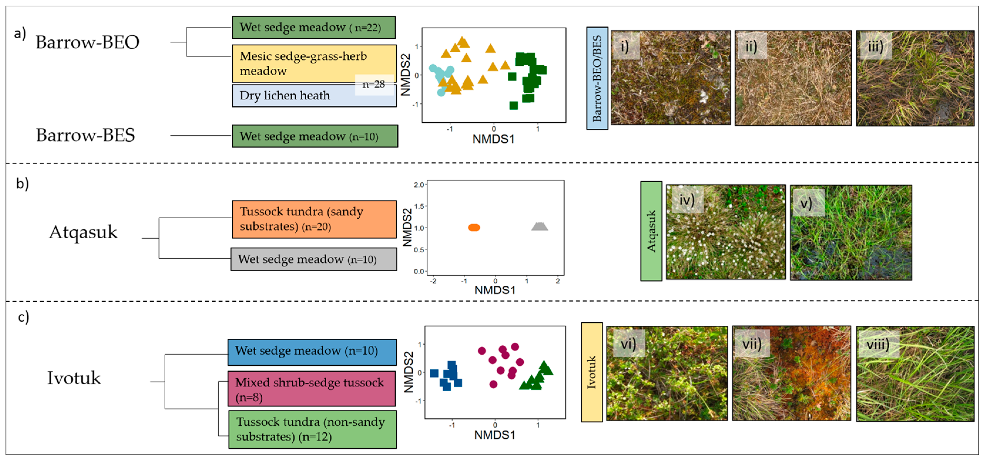
2.2. Vegetation Data

Vegetation surveys were conducted at the four tower sites between 18 and 31 July 2014. The main vegetation types and micro-topographic features (e.g., polygon troughs, rims and centers) were identified by an intensive walkover survey and use of previous vegetation maps of the areas [24,54] within a 300 m tower footprint, chosen as the “fetch”, i.e., the distance from the tower that carbon fluxes are expected to originate from, calculated as 100 m multiplied by the height of the tower (in this case, maximum tower height 3.5 m) [50,55]. A precautionary approach was taken during the vegetation survey by placing ten 1 m2 quadrats for which each vegetation type (wet sedge meadow for example) and feature was recorded. In total, this resulted in 5 vegetation types/50 quadrats at Barrow-BEO, 1 vegetation type/10 quadrats at Barrow-BES (which was only accessible from a central boardwalk), 2 vegetation types/30 quadrats (an additional 10 quadrats were placed in one type to capture the variability) at Atqasuk and 3 vegetation types over 30 quadrats at Ivotuk (Figure S1).
The percentage cover of all live vascular and non-vascular plant species and other materials including standing dead, standing water and bare ground was categorized as 0.1 (present), 1 (occasional, with 1 < x < 5 individuals), or 3 (containing more than 10 individuals). The nearest 5% of all live vascular, non-vascular and other materials thereafter were recorded. All vascular and nonvascular plant species identifications were made during the field campaign according to Hultén [56] and Vitt et al. [57] respectively.
For mapping purposes, dominant plant communities were defined using a combination of cluster analyses and ordination of species composition data. Groups of similar samples were identified using a one-way hierarchical cluster analyses performed using PC-ORD software version 6 (MjM Software, Gleneden Beach, OR, USA). Ordination was then performed using non-metric multi-dimensional scaling (NMDS) as this approach does not assume unimodal species response curves and is well suited to ecological datasets of this type [58]. The specifications used in the NMDS were selected according to the characteristics of the dataset and were: (i) Bray–Curtis distance measure; (ii) number of dimensions equals 2 (following examination of the stress plots of three runs); and (iii) data auto-transformation (Wisconsin double and square root transformations). The NMDS was performed in R version 3.1.0 (R Core Team 2014, [59]) using the VEGAN community ecology package [60]. The resulting plots for each site, on which samples are arranged primarily according to their floristic dissimilarity, were examined visually and compared with the groupings from cluster analysis.
For this analysis, classifications were conducted on the plant community level following the approach of Buchhorn et al. [28] and Bratsch et al. [39]. Although PFTs are commonly used in Earth System and other carbon flux models to prescribe vegetation parameters and system response to changing environmental conditions [61], the spatial heterogeneity of the tundra ecosystem is evident even at sub-meter scales, making single PFT classifications not good representatives of vegetation composition, distribution and properties. Furthermore, classifications based on landscape-level PFTs may result in higher classification errors at the tower footprint scale (~300–500 m) relative to classifications based on vegetation community type [28]. The vegetation community, chosen as the basis for our classification scheme, also better matches upscaling schemes used in local and regional carbon assessments, where land cover maps are used in conjunction with small area (e.g., 1 m chamber) flux measurements to obtain landscape level estimates of carbon exchange and greenhouse gas emissions [15]. Although the classifications resulting from this study do not directly reflect PFT types, our vegetation communities can be re-classified to PFT types for input in carbon flux models (in Section 3.2, a comparison of vegetation communities and PFTs is provided).

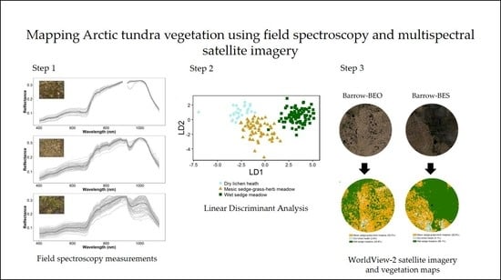
2.3. Field Spectroscopy Data Collection and Pre-Processing

Field spectroscopy measurements were collected using a UniSpec DC Spectrometer Analysis System (PP systems, Amesbury, MA, USA) having 256 discrete bands spanning from 450 nm to 1040 nm at the four field sites on a single occasion in July 2014 (Table 1). All measurements were collected under near to clear sky conditions and as close to solar noon as possible. For each vegetation type (Section 2.2), 30 spectral points were collected at quadrant locations matching the vegetation survey, within a 300 m radius footprint of the eddy covariance towers. In total, 150 samples were collected at Barrow-BEO (11 July 2014), 30 samples were collected at Barrow-BES (11 July 2014), 60 samples were collected at Atqasuk (29 July 2014), and 90 samples were collected at Ivotuk (16 July 2014) (Figure S1). Vegetation canopy reflectance was measured using downward facing fibre optic (UNI684 straight fibre optic, 2M, HCS LOH, SMA-custom ferrule with 100 mm tip) Hypo Tube (UNI688), which was used to control the field of view (FOV). Spectra were recorded from approximately 1.5 m above the ground with a FOV of 9.5°, corresponding to a circular surface with an approximate 50 cm diameter. A white standard (UNI240, PP systems, Amesbury, MA, USA) was used for white reference normalization. At each location, a photograph was taken to illustrate the vegetation community and a corresponding differential GPS measurement (dGPS) was acquired (Trimble R7, Trimble Navigation Limited, Sunnyvale, CA, USA).
As the field spectrometer used (UniSpec DC) did not account for incoming radiation, the raw spectral data was corrected using the mean white reference standard normalization measurement taken during each measurement period. One mean reflectance spectrum for each vegetation community (calculated from between 30 and 60 spectral measurements dependent on vegetation community characteristics and sampling quality) was calculated per location. Wavebands that fell outside the range of 450–1040 nm in the raw reflectance data (hereby referred to as UniSpec) were removed during quality control processing. The UniSpec data were then rescaled to match the 7 bands of the WorldView-2 satellite data (hereby referred to as UniSpecWV2) to test whether downgrading narrowband data to multispectral data would still produce accurate tundra vegetation maps. We degraded the UniSpec data to the 7 WorldView-2 bands by averaging band reflectance as follows: Blue: 450–510 nm; Green: 510–580 nm; Yellow; 585–625 nm; Red: 630–690 nm; Red Edge: 705–745 nm; NIR1: 770–895 nm; and NIR2: 860–1040 nm.

2.4. Satellite Data Collection and Pre-Processing

The WorldView-2 multispectral data (2 m spatial resolution) acquired for Barrow-BEO and Barrow-BES, Atqasuk and Ivotuk were also used to classify tundra vegetation (Table 1). The image acquisition dates were selected for the time period between vegetation sampling and field spectral measurement campaigns. All sites had imagery for 2014 with the exception of Ivotuk, where imagery from 2013 was used as there was no suitable, cloud-free satellite imagery available during the following year. The orthorectified WorldView-2 data were georeferenced and calibrated to Top-of-Atmosphere Reflectance following the procedures outlined by Digital Globe (Digital Globe Corporate. Longmont, CO, USA). To assess whether we could relate the TOA reflectance to the spectrometer data we used a dark object subtraction and then compared reflectance values at known locations (see Supplementary Material for a detailed description). We extracted the reflectance data from the WorldView-2 satellite imagery using dGPS locations of the field spectrometry measurements (extracted data is hereby referred to as WorldView-2). The spatial accuracy of georeferenced dGPS points was within 30 cm of “truth” using the satellite imagery.

2.5. Vegetation Indices

We used the UniSpec, UniSpecWV2 and WorldView-2 reflectance data to calculate three vegetation indices (VIs), namely the normalized difference vegetation index (NDVI) [62], the normalized difference water index (NDWI) [63] and the enhanced vegetation index (EVI) [64]. We chose these indices as NDVI is commonly used to describe the quantity of green vegetation at plot and landscape levels [25,29,65]. The EVI was included to improve on areas where NDVI is limited, due to canopy structure variation [64,66], i.e., non-homogeneous Arctic tundra vegetation can range from <1 cm to >5 m in height therefore affecting the reflectance signal, and sensitivity to background reflectance from soils, etc. [67]. The NDWI estimates plant water stress and associated impacts on plant productivity, phenology, and land cover classifications. This is especially useful in Arctic tundra ecosystems where water table depth and soil moisture can be intrinsically linked to vegetation cover [37,68]. We used the field spectroscopy bands 665 nm and 845 nm [69] and the Red and NIR1 from the UniSpecWV2 and WorldView-2 data to calculate NDVI, NDWI and EVI. The advantage of using vegetation indices in combination with raw reflectance data is that the indices themselves relate parts of the spectra to reflect biochemical properties and other properties of the spectra that cannot be accounted for when analyzing each individual band.

2.6. Spectral Separability and Image Classification

Our objective was to map the following vegetation communities: mesic-sedge-grass-herb meadow, dry lichen heath, wet sedge meadow, tussock tundra, and mixed shrub-sedge tussock tundra. These were the vegetation community classes resulting from the vegetation clustering analysis (described in Section 3.1). We first tested whether there was adequate spectral separability among tundra vegetation communities to inform a classification algorithm to produce a vegetation map. To do this, we applied a Principal Component Analysis (PCA) to UniSpec data to assess whether the vegetation communities were separable. The PCA identifies whether each vegetation community is in a different area of the reflectance data space, and the loadings of the PCA axes indicate the contribution of reflectance at each of the spectral bands to the final PCA plot [69]. Secondly, we used a one way analysis of variance (ANOVA) and a pair-wise post hoc Tukey HSD test (95% confidence level) to assess which wavelengths differed significantly among the vegetation communities. Once the region(s) were defined, a second PCA was used on the selected wavelengths.
Finally, we used a linear discriminant analysis (LDA) to discriminate amongst the vegetation communities. We chose this method because it allows for the identification of significant differences among groups based on relatively large numbers of variables [70], through variable reduction to linear combinations of those variables that explain the majority of variation in the data [71]. It has been successfully used to classify vegetation communities and species in several studies [41,72,73], including tundra [39]. We classified the communities using input UniSpec data from the significantly different wavelengths, as well as the UniSpecWV2 reflectance and WorldView-2 image reflectance data. We also trained a LDA using a combination of each type of reflectance data and the three VIs. Initially, one classifier was developed across-sites, but this was deemed unsuitable due to low classification accuracies (see Supplementary Material, Figure S3), therefore site-specific classifiers were developed. Two LDA functions were obtained from each analysis, producing three classes each for Barrow-BEO/Barrow-BES and Ivotuk and two classes for Atqasuk.
Classification accuracy was calculated as the number of ground truth points correctly classified in a given vegetation community divided by the number actually in that reference vegetation community. The Kappa coefficient metric [74] was used as a statistical measure summarizing the classification accuracy. Kappa coefficient values range from −1 to 1, with ≤0 indicating no agreement, and 0.01–0.20 as none to slight, 0.21–0.40 as fair, 0.41–0.60 as moderate, 0.61–0.80 as substantial and 0.81–1 as almost perfect agreement [74].
We applied the resulting LDA discriminant functions (UniSpecWV2 and UniSpecWV2 plus VI) to the seven WorldView-2 bands to produce the final vegetation community map for each field site. For each image we ran all the corresponding LDA functions (as many as number of vegetation communities at the site), and images were classified with 4–6 classes. As only two of the many communities found at Atqasuk [75] were found in the tower footprint, one resulting LDA function was produced. Finally, the LDA maps were combined by layering each raster together and the final vegetation classes were mapped. Pair-wise error matrices (and corresponding Kappa coefficients) for each analysis type (LDA including or excluding VIs) and site were calculated based on errors of omission and commission between the classified maps and the ground-truth data. Analysis was undertaken using ENVI v5.2 (Exelis Visual Information Solutions, Boulder, CO, USA) and ArcMap v.10.2.1 (ESRI 2011. ArcGIS Desktop, Environmental Systems Research Institute, Redlands, CA USA). All statistical analyses were carried out using the packages CRAN and MASS in R version 3.1.0 (R Core Team 2014) [59].

3. Results

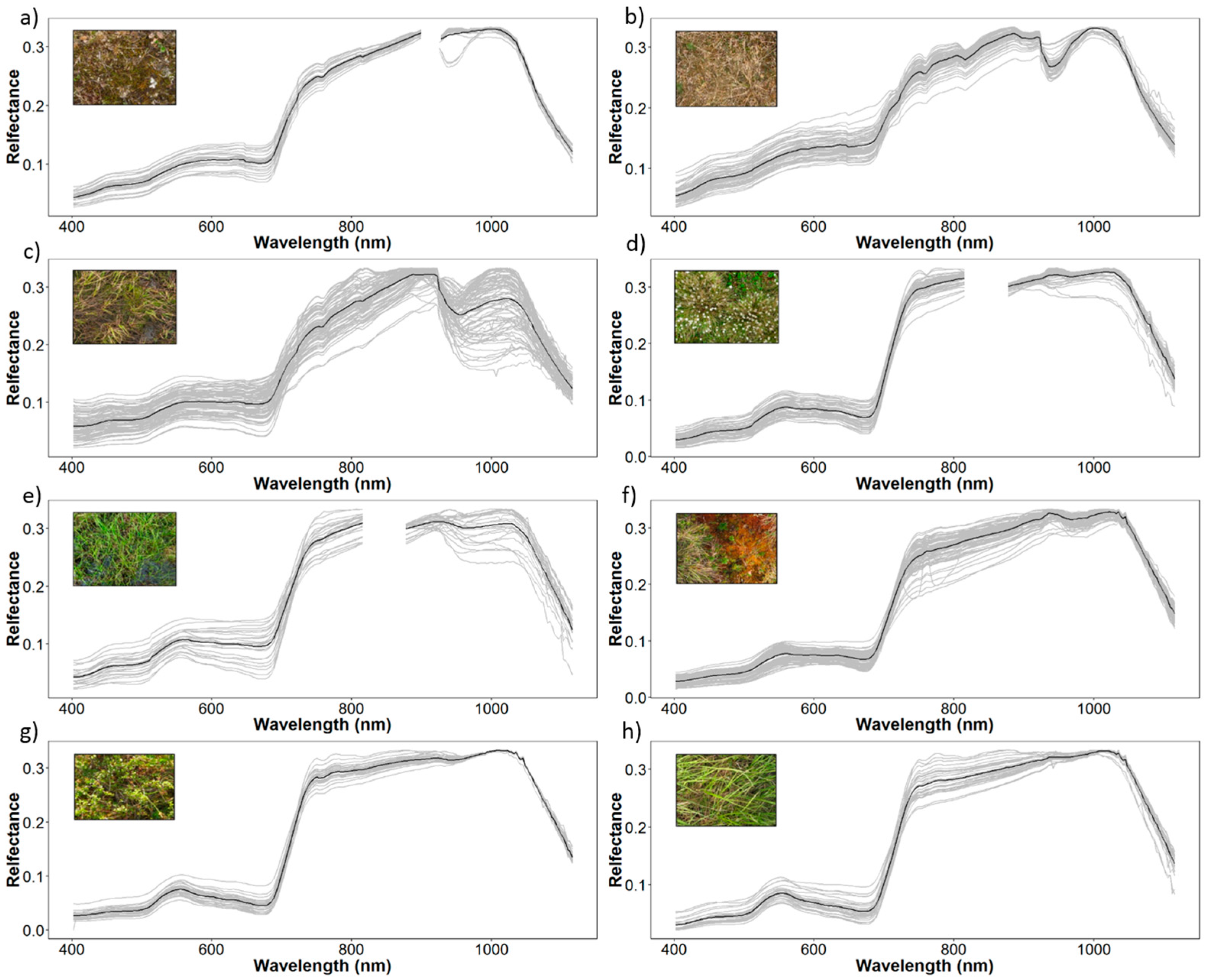
3.1. Vegetation Communities

Hierarchical one-way clustering and NMDS analysis showed a total of eight close groupings, including mesic-sedge-grass-herb meadow, dry lichen heath, wet sedge meadow, tussock tundra (two separate communities at Atqasuk (sandy substrates) and Ivotuk (non-sandy substrates), and mixed shrub-sedge tussock tundra communities (Figure 2).
At Barrow-BEO/Barrow-BES, the dry lichen heath community was dominated by Polytrichum moss and various lichen species, with little vascular plants present, while the mesic-sedge-grass herb meadow community was dominated by a mixture of graminoid species (Eriophorum russeolum and Poa arctica) with various mosses, lichens and liverworts present. The wet sedge community here was dominated by Carex aquatilis (sedge) with an underlying Sphagnum spp. and Drepanocladus spp. moss carpet below the canopy. At Atqasuk, the tussock sedge (sandy substrates) community was dominated by Eriophorum vaginatum, Aulocomnion turgidum, Rubus chamaemorus and various evergreen shrubs. The wet sedge community here does not contain a moss layer, but consisted of Eriophorum angustifolium and Eriophoporum russeolum. At Ivotuk, the tussock sedge (non-sandy substrates) also contained Eriophorum vaginatum tussocks interspersed with Sphagnum spp., as well as various evergreen and deciduous shrubs. The wet sedge community here consisted of tall Carex aquatilis, with low-growing deciduous shrubs such as Salix pulchra and a moss carpet containing Sphagnum spp. The mixed shrub-sedge tussock community was also dominated by large Salix pulchra and Betula nana, with Eriophorum vaginatum tussock. Details on species frequency and abundance are provided in Supplementary Material (Table S1) and details on PFT frequency and abundance within all eight communities are provided in Table 2.

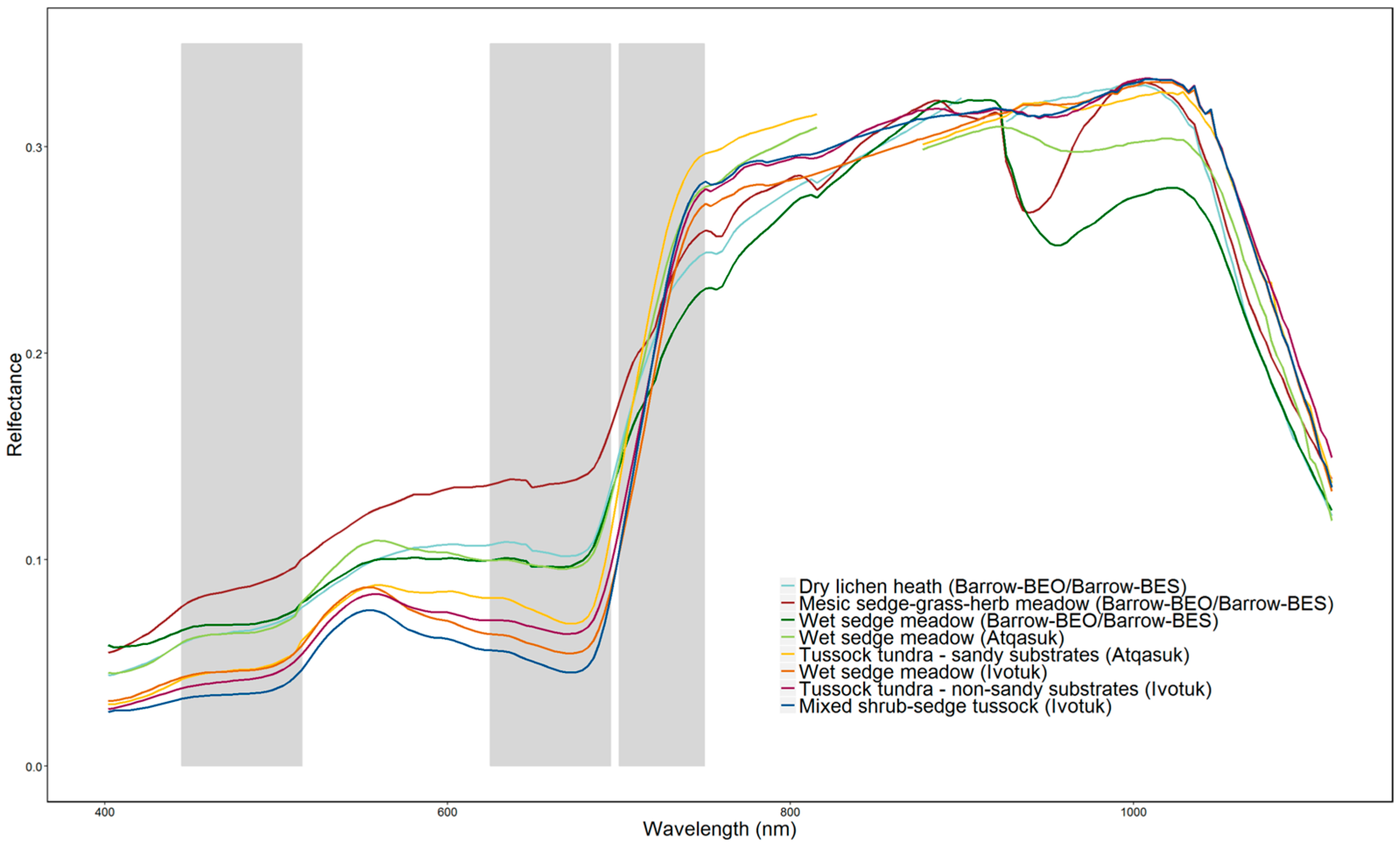
3.2. Spectral Separability in Tundra Vegetation Communities

Average spectral profiles for all vegetation communities are shown in Figure 3. Vegetation communities differed in the shape of their spectral signature in the visible region of the spectrum, mostly due to the mesic sedge-grass-herb meadow and dry lichen heath communities showing higher reflectance in the green (about 10%, at 600 nm) and in the red (about 12%, at 680 nm) regions relative to the other vegetation communities. Communities differed in the NIR region, with the wet sedge meadow community (Barrow-BEO/Barrow-BES) showing much lower reflectance (around 25%), followed by the mesic sedge-grass-herb meadow and wet sedge meadow (Atqasuk) communities (between 24% and 28%, respectively). The other communities showed similar reflectance values in the NIR region. Mesic sedge-grass-herb meadow and wet sedge tundra has a characteristic water absorption feature at ~970 nm, likely from the large amount of standing water (between 30% and 80% coverage; Table 2).
Vegetation communities varied significantly in spectral characteristics across the four tower sites. The mixed shrub-sedge tussock tundra (Ivotuk) was generally not separable from mesic sedge-grass herb meadow in the Near-IR2 (Table 3). Tukey’s HSD tests (Table S2) showed that the mesic sedge-grass herb meadow community had significantly higher reflectance in the blue (7%, 450–510 nm), red (12%, 630–690 nm) and red edge (23%, 705–745 nm) regions (Figure 4), while mixed shrub-sedge tussock had the lowest reflectance (3%, 5% and 11%, respectively). Dry lichen heath and wet sedge meadow had similar reflectance in the blue spectrum (approximately 8%), but dry lichen heath had higher reflectance in the red (16% compared to 12%) and lower in the red-edge (23% compared to 26%). Tussock tundra (non-sandy substrates), wet sedge meadow (Ivotuk) and mixed shrub-sedge tussock had the lowest reflectance in the blue (4%, 4% and 3%, respectively), but were differentiable in the red, and tussock tundra (sandy substrates; Atqasuk) had the highest reflectance in the red-edge (29%).

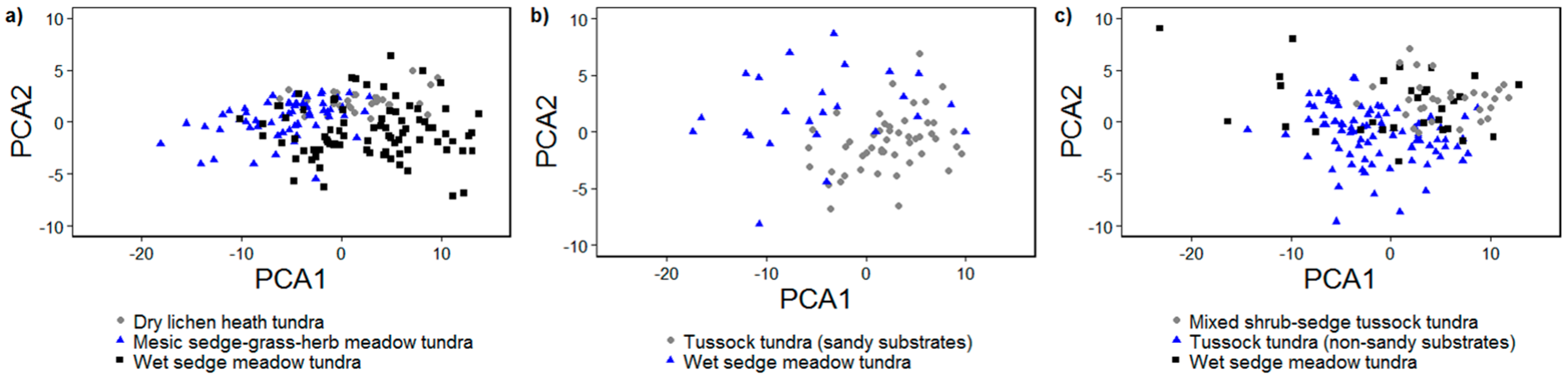
3.2.1. Principal Components Analysis

The PCA using UniSpec data at all four sites showed limited separability between vegetation communities, with 48.9% of the variation in the data being explained by the first component alone, and 70.2% explained by the first two components (Figure S2). At the individual site level and using the three significant regions (blue, red and red edge), the PCA showed much higher community separability (Figure 5). Communities at Atqasuk had clearer separation than at the other sites (Figure 5b). For Barrow-BEO/Barrow-BES, 93.3% of the variation in the data was explained by the first component alone, and 99.7% was explained by the first two components. For Ivotuk, 67.9% of the variation was explained by the first component and 86.5% was explained by the first two components. For Atqasuk, 74.9% and 94.8% of the variation was explained by the first component and the first two components, respectively.
The regions of the spectrum that most contributed to PCA1 at Barrow-BEO/Barrow-BES and Atqasuk were blue, red and red edge; red edge (450–510, 630–690 and 705–745 nm, respectively) contributed most to PCA2 at both Barrow-BEO/Barrow-BES and Atqasuk. At Ivotuk, it was only the blue and red, which contributed most to PCA1 and red edge contributed most to PCA2.

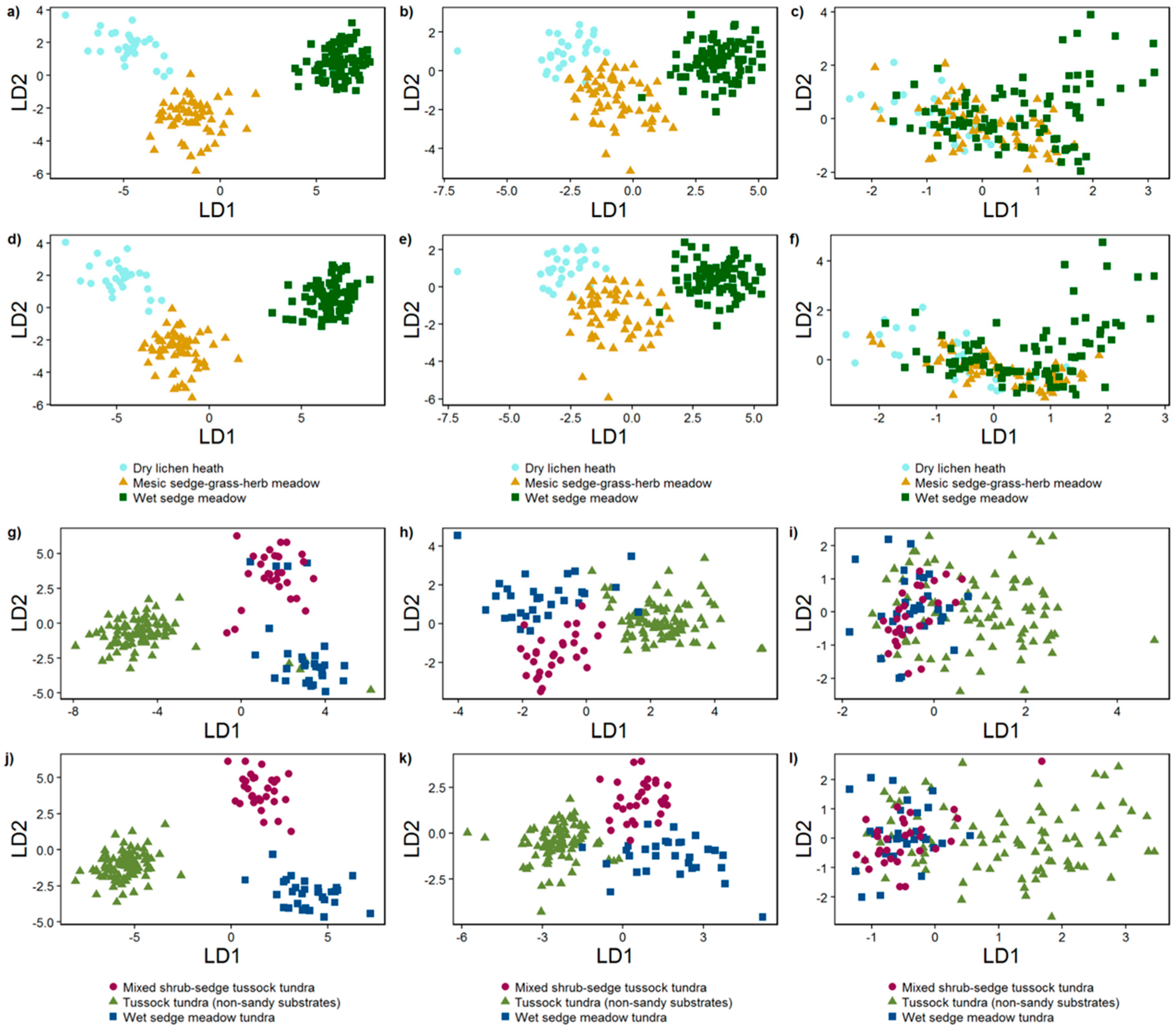
3.2.2. Linear Discriminant Analysis

Due to the high variability across the field sites, site-specific classifiers were required as we found one classifier to be inadequate for characterizing all classes across the tower sites (see Supplementary Material; Figure S4).
The individual LDA results for the UniSpec and UniSpecWV2 data across all sites showed minimal overlap in the vegetation communities (Figure 6a,b,d,e,g,h,j,k). This discrimination was achieved with accuracies between 90% and 100% (Kappa coefficients ranging between 0.86 and 1; Table 4, Figure 7) for the UniSpecWV2 data. Adding NDVI, NDWI and EVI further improved the results, resulting in classification accuracies between 90% and 100% (Kappa coefficient values ranging between 0.88 and 1; Table 4, Figure 7).
At Barrow-BEO/Barrow-BES and Ivotuk, the WorldView-2 data resulted in low classification accuracies, ranging between 50% and 64% (Kappa coefficient values of between 0.24 and 0.37; Table 4). Adding the vegetation indices resulted in an equally poor classification, with accuracies ranging between 39% and 67% (Kappa coefficient values between 0.26 and 0.4). Atqasuk, however, had results similar to the UniSpecWV2 data, with classification accuracies ranging between 86% and 92% (Kappa coefficient values between 0.71 and 0.74; Table 4).

3.2.3. Vegetation Map Validation

Higher classification accuracy was achieved when using the UniSpecWV2 reflectance data to classify dry lichen heath, wet sedge meadow (Barrow-BEO/Barrow-BES) and tussock tundra (sandy substrates). Vegetation community classification accuracies between each classifier varied quite considerably. At Barrow-BEO and Barrow-BES, using the LDA function from the UniSpecWV2 reflectance data (including three VIs) improved classification accuracy for both the mesic sedge-grass-herb meadow and dry lichen heath, yet decreased the accuracy for the wet sedge community (Table 5). The overall classification accuracy for these two sites was 65% (Kappa coefficient 0.43) without VIs and 64% (Kappa coefficient 0.43) including VIs.
At Atqasuk, including VIs in the LDA decreased accuracy for the tussock tundra (sandy substrates) community, but increased it for the wet sedge community (Table 5). The overall classification accuracies for both techniques were 88% (Kappa coefficient 0.71) and 80% (Kappa coefficient 0.56), respectively.
At Ivotuk, an improvement in the classification results occurred when including VIs for both the wet sedge meadow and the mixed shrub-sedge tussock communities, but a decrease in accuracy occurred for the tussock tundra (non-sandy substrates) (Table 5). The overall classification accuracies for both techniques were 67% (Kappa coefficient 0.39) and 73% (Kappa coefficient 0.52), respectively.
The LDA results using the UniSpecWV2 reflectance data showed little variation in vegetation community distribution, with Barrow-BEO and Barrow-BES showing a 92% agreement between with or without inclusion of VIs. Atqasuk showed a little more variation, with 78% agreement using the rescaled data, between either including or excluding VIs. Finally, Ivotuk had similar accuracy using the UniSpecWV2 reflectance data, with 77% agreement in vegetation community distribution. Vegetation community distributions (percentage cover of the tower footprint area) using both analyses techniques are shown in Table 6 and finalized maps are shown in Figure 7.

4. Discussion

This study demonstrates that it is possible to successfully distinguish between the dominant vegetation communities at the four Alaska tundra tower field sites using a combination of the blue, red and red edge regions of the electromagnetic spectrum obtained from UniSpec and UniSpecWV2 data. Furthermore, using UniSpec bands within a LDA, successful discrimination between tundra vegetation communities was achieved with classification accuracies between 83% and 98%. These results were used to map tundra vegetation communities within the flux tower footprints using 2 m resolution WorldView-2 imagery. However, we were not able to produce high accuracy (classification accuracies over 80%) vegetation maps for 300 m tower footprints using the same classifier at all four sites due to the sub-pixel heterogeneity of the land cover [76]. Finally, scaling from plot (e.g., UniSpec) to landscape (WorldView-2) was challenging because of the difference in spatial resolution between the field spectroscopy narrow band reflectance data and the multispectral satellite imagery. These results indicate that multispectral satellite imagery having a spatial resolution of 2 m is not spatially adequate to represent the innate sub-meter vegetation heterogeneity found in these ecosystems as described by Muster et al. [76]. Furthermore, spectral aggregation could also be a factor. For example, even if a pixel contained a homogenous vegetation community, there will inherently be a loss of spectral information when aggregating spectral data across a wider bandwidth.
Using the UniSpec data, the Arctic tundra vegetation communities were separable from a spectral perspective, in particular within the blue, red and red edge regions of the spectrum, which is in agreement with other studies having similar vegetation communities [4,28,39]. Although spectral profiles of the primary vegetation community types (wet sedge meadow, tussock tundra, etc.) showed certain diagnostic reflectance and absorption features, it can be challenging to distinguish between community spectral signatures [28,77]. In this study, we were not able to distinguish between community spectral signatures using all bands, but obtained successful separation between community spectral signatures in the blue, red and red edge regions. The blue and red regions can be linked to light absorption by plants, while the red edge region (680–740 nm) can be a useful metric of chlorophyll content [78]. These regions are a useful metric for the vitality of vegetation, while the short-wave infra-red region can be especially useful in tundra ecosystems, as the reflectance of vegetation such as the dry lichen heath communities are influenced by absorption of cellulose and lignin in this region, as well as reduced absorption by water and chlorophyll [79]. This creates a spectral signature that is distinguishable in comparison to green, vascular vegetation, which is shown in our results. Previous studies have also shown high NIR backscatter in the reflectance spectra of shrub tundra communities with decreased slope between beginning and end of NIR reflectance plateau [28]. Additionally, both wet sedge and tussock sedge communities in this study show NIR reflectance plateaus with stronger slopes between beginning and end of plateaus.
The mesic sedge-grass-herb meadow and dry lichen heath had a high proportion of low-chlorophyll-rich species, high non-vascular plant cover and higher proportion of dead plant material, which corresponds to lower reflectance in the blue and green regions and higher reflectance in the red region. This is highlighted by Buchhorn et al. [28], who show that areas with higher dead plant material also had limited development of a green reflectance peak due to reduced leaf pigment absorption. Arguably the “greenest” and most productive vegetation, the mixed shrub-sedge tussock community at Ivotuk, had the deepest chlorophyll absorption. Buchhorn et al. [28] also highlight that spectral behavior in the NIR region is intrinsically linked with soil moisture and mean vegetation height. At our study sites, the community with lowest reflectance within the NIR region was the wet sedge meadow at Barrow-BEO/Barrow-BES which had high surface moisture content as well as having tall sedges present.
The classification results in this study may have been affected by mixed signals caused by standing water, different species, soil surface features and moisture content of surrounding vegetation and soil [79]. Within certain communities (for example, the wet sedge meadow at Barrow-BEO/Barrow-BES) there was a substantial amount of open water when the measurements were taken, therefore leading to “noise” in the spectral signal. Furthermore, the structure of the tussock sedge communities can also impact the reflectance, as their erectophile structure, along with high density of dead plant material may cause additional backscattering in the NIR region [80]. Schaepman-Strub et al. [77] highlight there can be limitations when trying to obtain fractional cover of graminoid and shrub-dominated communities within peatlands. The fine-scale differences between the plant traits, community dynamics and spectral properties create the unique spectral signatures that allow each community to be differentiated. This can be especially useful as many areas of the Arctic are undergoing an increase in shrub-cover [13], allowing for potential mapping of this expansion, as well as partitioning vegetation community contribution to landscape level carbon budgets.
Adding VIs improved classification accuracy as they reduce spectral noise and can be directly related to plant physiology [45], and therefore linked to detailed arctic tundra vegetation properties [81]. VIs have shown that the simple transformation of band reflectance can be less sensitive to external variables [45], subsequently producing potentially more accurate classifications for heterogeneous landscapes over large areas. The improved performance when including VIs in this study is especially useful in regards to monitoring plant productivity and ecosystem functioning. It has been shown previously [82,83] that NDVI can be linked heavily with net ecosystem exchange (NEE) [84,85] and CH4 fluxes [25] for example. NDVI can be highly correlated with vegetation leaf area index (LAI), but also is invariant at higher LAI ranges and can be very sensitive to background variations in vegetation communities such as background soil and water [8]. The inclusion of the EVI and NDWI in our analysis improved classification accuracies across the majority of sites, as they allow for more detailed analysis of canopy structure variation [64] and plant water stress/soil water content [37], respectively.
Higher accuracy classifications (between 92% and 96%) occurred from the UniSpecWV2 data. These results suggest that it is possible for remotely-sensed tundra vegetation to be scaled from plot (<1 m) to the patch (~500 m) scale due to the reduced noise in the signal found in the extracted data, allowing for better separation between communities. The UniSpecWV2 reflectance data was used to produce the maps of the Arctic tundra vegetation with and without inclusion of VIs (classification accuracies for Barrow-BEO/Barrow-BES, 65% and 64%; Atqasuk, 88% and 80%; and Ivotuk, 67% and 73%, respectively). Although the classifier used in the analysis (with input UniSpecWV2 data) was obtained using narrow band field spectroscopy data rescaled to match the broad bands of the satellite imagery, they still maintain a level of accuracy that is found when using the narrow bands (>80% accuracy). However, at the individual field sites, classification accuracies were lower, possibly due to mixed signals caused by the heterogeneous nature of the vegetation communities, with spectral characteristics in each reflecting a combination of different vegetation communities within the 2 m resolution of each pixel. Where individual community separation was less successful, this could be due to the heterogeneous nature of the land cover. For example, at Ivotuk, the wet sedge meadow contains some areas having substantial shrub cover, causing a mixing of the spectral signature [78], with both communities showing similar spectral signatures, especially in the red edge region. Kushida et al. [86] showed no significant difference between sedge and shrub plots located at an Alaskan study site, even though both communities have very different structural properties. At first glance, many of the tundra communities evaluated in this study appeared similar, containing similar species. However, at the spectral level they were significantly different. For example, the mesic sedge-grass-herb meadow and dry lichen heath tundra communities at Barrow-BEO/Barrow-BES and the tussock tundra communities at both Atqasuk and Ivotuk could be considered physiognomically similar respectively, due to the communities containing similar species/abundance, yet they differed significantly when evaluating the spectral profiles. This could be due to the proportions of non-vascular plant species in the dry lichen heath community in comparison to the mesic-sedge-grass-herb meadow, which have an impact on the spectral signal [3]. The spectral reflectance of non-vascular communities is influenced by absorption of cellulose and lignin (and lack of absorption by chlorophyll as found in “green” vascular plant communities [79].
The results of the LDA using the WorldView-2 data indicate a loss in classification accuracy. This again highlights the “ecologically complex” nature of land cover across these field sites, with the 2 m satellite imagery resolution being insufficient to capture the fine-scale heterogeneity in vegetation cover. However, Atqasuk showed similar classification accuracies between using the UniSpecWV2 and WorldView-2 data. This may be due to only having two dominant communities at this site, therefore the landscape is much less heterogeneous, with each community being spectrally different from one another. Vegetation across these landscapes ranged from short stature communities in the high Arctic, to communities containing larger shrubs and tussock sedges as one moves further south and with varying levels of moisture, all linked to further ecosystem processes. This may have resulted in the inability to produce an all-site classifier, due to the lack of representation of all vegetation communities at each site. However, the vegetation communities described in this study are representative of large areas across the Alaskan Arctic. The spatial heterogeneity of vegetation communities across these landscapes means they may contribute differently to the landscape-scale carbon exchange [77,87], highlighting the necessity to be able to map vegetation communities at a fine-scale. Therefore, the classifiers created are valuable with regards to their ability to map fine-scale vegetation communities.
One limitation to the research presented here is there is no temporal aspect to the vegetation maps, as they are created using data collected at one time period during 2014 (satellite imagery for Ivotuk was obtained in 2013 due to no suitable imagery available for 2014). The microclimatic differences in climate (from year to year), hydrology and topography can influence vegetation community composition and biomass/greenness [12,88,89]. Therefore, data should be collected within a suitable time period (ideally within the same year/month) during the growing season so it is as representative as it can be of the community present [89]. However, changes in Arctic vegetation community composition occurs at a slower rate than elsewhere due to low temperatures and short growing seasons, and the vegetation communities found in these locations could be considered “stable”, with the distribution of each community unlikely to change rapidly enough to make the findings of this study non-applicable. Even if the communities are not stable [88,90], the growth rate is so slow that it still makes the study applicable across a short time span like the difference in data collection dates at Ivotuk. Potential expansion of wet sedge meadow communities could occur with further permafrost thaw with areas becoming wetter [91,92] over a decadal time scale [93], but we believe the vegetation maps created within this study were likely not majorly affected by the temporal variation across these sites, making them applicable for using within carbon cycle prediction models. Given the substantial cloud cover of these arctic ecosystems, previous studies (including Langford et al. [47] have used imagery and ground truthing data collected in different years. Ideally the use of airborne hyperspectral imagery [19] or unmanned aerial vehicles (UAV) with very high spatial resolution (sub-centimeter for UAV), collected at the same time of ground data will improve the accuracy of vegetation mapping, especially at the patch scale [94]. In addition, airborne LiDAR [47] might also be used to improve classification accuracies by providing data of vegetation structure and biomass profiles, in addition to terrain features that may influence landscape temperature and moisture conditions and consequently vegetation characteristics.

5. Conclusions

We show that field spectroscopy can be used to successfully discriminate and map dominant tundra vegetation communities for four sites in northern Alaska. The vegetation communities found at Ivotuk represents the dominant tundra vegetation type in Alaska, while communities at Barrow and Atqasuk represent approximately 60% of all Arctic wetlands [23]. In this study, these vegetation communities were classified with patch scale (~500 m) accuracies ranging from over 50% to 80%. This highlights the applicability and representativeness of this methodology for mapping these heterogeneous environments at this scale. There are however, limitations to scaling up and mapping tundra vegetation communities because of the requirements for high spatial resolution satellite or airborne data across the landscape. This study highlights the benefits of using fine-scale spectroscopy over coarse areas (300 m eddy covariance tower footprints) for tundra vegetation classification and demonstrates the ability to map vegetation communities using field spectroscopy in combination with high spatial resolution multispectral satellite imagery. Although coarse scale vegetation mapping across Arctic tundra ecosystems is suitable for broad-scale vegetation distribution monitoring, there is still a necessity to include fine-scale vegetation community mapping in further carbon cycle models in order to accurately assess their influence, thus facilitating the monitoring of changes occurring as a result of a warming Arctic and understanding large scale ecological processes in Arctic plant community assemblage.

Supplementary Materials

The following are available online at www.mdpi.com/2072-4292/8/12/978/s1, Supplementary material Section 1: Description of Dark Object Subtraction; Figure S1: Regression of reflectance at known locations before and after dark object subtraction. Reflectance at all bands was strongly correlated showing that the TOA reflectance can be compared with in situ reflectance, Figure S2: Maps showing spatial locations of the vegetation community analysis and field spectroscopy survey points within the eddy covariance tower footprints, Figure S3: Principal component analysis of UniSpec DC reflectance data using all narrow bands; Figure S4: Linear Discriminant Analysis (LDA) plots, Table S1: Floristics table of all vegetation communities. Species list is ordered by frequency across all quadrats. Data are frequency (I–V) within each community and abundance range (% cover). Quadrats per community = (however many in the smallest group to however many in the largest group); Table S2: Tukey HSD Comparison for each vegetation community and WorldView-2 multispectral imagery bands.

Acknowledgments

This work was funded by the Office of Polar Programs of the National Science Foundation (NSF) awarded to DZ (award number 1204263) with additional logistical support funded by the NSF Office of Polar Programs, and Carbon in Arctic Reservoirs Vulnerability Experiment (CARVE), an Earth Ventures (EV-1) investigation, under contract with the National Aeronautics and Space Administration. Additional funding was provided by a Royal Society International Exchange (2013/R1), and a NERC Arctic Research Programme, CYCLOPS Grant (NE/K00025X/1) to GKP. SJD is supported by a NERC PhD studentship. This research was conducted on land owned by the Ukpeagvik Inupiat Corporation (UIC). We would like to thank the Global Change Research Group at San Diego State University in particular Patrick Murphy and UMIAQ and UIC for logistical support Ali Hoy, and Owen Hayman for the help in the field. We would like to thank Cole Kelleher and the team at the Polar Geospatial Centre at the University of Minnesota for their help with the satellite imagery.

Author Contributions

D.Z., W.C.O., and G.K.P. secured the funding; S.J.D., M.J.S., V.L.S., D.Z., W.C.O., and G.K.P. designed the study; S.J.D., V.L.S. and J.D.W. performed the research; S.J.D. and M.J.S. analyzed the data with input from V.L.S., D.Z. and G.K.P.; and S.J.D., M.J.S., V.L.S., G.K.P, J.D.W., W.C.O. and D.Z. wrote the paper.

Conflicts of Interest

The authors declare no conflict of interest.

References

  1. Oechel, W.C.; Vourlitis, G.L.; Hastings, S.J.; Zulueta, R.C.; Hinzman, L.; Kane, D. Acclimation of ecosystem CO2 exchange in the Alaskan Arctic in response to decadal climate warming. Nature 2000, 406, 978–981. [Google Scholar] [CrossRef] [PubMed]
  2. Chapin, F.S.; Sturm, M.; Serreze, M.C.; McFadden, J.P.; Key, J.R.; Lloyd, A.H.; McGuire, A.D.; Rupp, T.S.; Lynch, A.H.; Schimel, J.P.; et al. Role of land-surface changes in arctic summer warming. Science 2005, 310, 657–660. [Google Scholar] [CrossRef] [PubMed]
  3. Huemmrich, K.F.; Gamon, J.A.; Tweedie, C.E.; Entcheva Campbell, P.K.; Landis, D.R.; Middleton, E.M. Arctic tundra vegetation functional types based on photosynthetic physiology and optical properties. IEEE J. Sel. Top. Appl. Earth Obs. Remote Sens. 2013, 6, 265–275. [Google Scholar] [CrossRef]
  4. Huemmrich, K.F.; Gamon, J.A.; Tweedie, C.E.; Oberbauer, S.F.; Kinoshita, G.; Houston, S.; Kuchy, A.; Hollister, R.D.; Kwon, H.; Mano, M.; et al. Remote sensing of tundra gross ecosystem productivity and light use efficiency under varying temperature and moisture conditions. Remote Sens. Environ. 2010, 114, 481–489. [Google Scholar] [CrossRef]
  5. Zeng, H.; Jia, G.; Epstein, H. Recent changes in phenology over the northern high latitudes detected from multi-satellite data. Environ. Res. Lett. 2011, 6, 45508–45518. [Google Scholar] [CrossRef]
  6. Ju, J.; Masek, J.G. The vegetation greenness trend in Canada and US Alaska from 1984–2012 Landsat data. Remote Sens. Environ. 2016, 176, 1–16. [Google Scholar] [CrossRef]
  7. Starr, G.; Oberbauer, S.F.; Ahlquist, L.E. The photosynthetic response of Alaskan tundra plants to increased season length and soil warming. Arct. Antarct. Alp. Res. 2008, 40, 181–191. [Google Scholar] [CrossRef]
  8. Walker, D.A.; Jia, G.J.; Epstein, H.E.; Raynolds, M.K.; Chapin, F.S., III; Copas, C.; Hinzman, L.D.; Knudson, J.A.; Maier, H.A.; Michaelson, G.J.; et al. Vegetation-soil-thaw-depth relationships along a low-arctic bioclimate gradient, Alaska: Synthesis of information from the ATLAS studies. Permafr. Periglac. Process. 2003, 14, 103–123. [Google Scholar] [CrossRef]
  9. Tape, K.; Sturm, M.; Racine, C. The evidence for shrub expansion in Northern Alaska and the Pan-Arctic. Glob. Chang. Biol. 2006, 12, 686–702. [Google Scholar] [CrossRef]
  10. Myers-Smith, I.H.; Forbes, B.C.; Wilmking, M.; Hallinger, M.; Lantz, T.; Blok, D.; Tape, K.D.; Marcias-Fauria, M.; Sass-Klassen, U.; Lévesque, E.; et al. Shrub expansion in tundra ecosystems: Dynamics, impacts and research priorities. Environ. Res. Lett. 2011, 6, 1–15. [Google Scholar] [CrossRef]
  11. Serreze, M.C.; Walsh, J.E.; Chapin, F.S., III; Osterkamp, T.; Dyurgerov, M.; Romanovsky, V.; Oechel, W.C.; Morison, J.; Zhang, T.; Barry, R.G. Observational evidence of recent change in the northern high-latitude environment. Clim. Chang. 2000, 46, 159–207. [Google Scholar] [CrossRef]
  12. Zona, D.; Lipson, D.A.; Richards, J.H.; Phoenix, G.K.; Liljedahl, A.; Ueyama, M.; Sturtevant, C.S.; Oechel, W.C. Delayed responses of an Arctic ecosystem to an extreme summer: Impacts on net ecosystem exchange and vegetation functioning. Biogeosciences 2014, 11, 1–12. [Google Scholar] [CrossRef]
  13. Zhang, W.; Miller, P.A.; Smith, B.; Wania, R.; Koenigk, T.; Döscher, R. Tundra shrubification and tree-line advance amplify arctic climate warming: Results from an individual-based dynamic vegetation model. Environ. Res. Lett. 2013, 8, 1–10. [Google Scholar] [CrossRef]
  14. King, J.Y.; Reeburgh, W.S.; Regli, S.K. Methane emission and transport by arctic sedges in Alaska: Results of a vegetation removal experiment. J. Geophys. Res. 1998, 103, 29083–29092. [Google Scholar] [CrossRef]
  15. Davidson, S.J.; Sloan, V.L.; Phoenix, G.K.; Wagner, R.; Fisher, J.P.; Oechel, W.C.; Zona, D. Vegetation type dominates the spatial variability in CH4 emissions across multiple Arctic tundra landscapes. Ecosystems 2016, 19, 1116–1132. [Google Scholar] [CrossRef]
  16. Stow, D.A.; Hope, A.; McGuire, D.; Verbyla, D.; Gamon, J.; Huemmrich, F.; Houston, S.; Racine, C.; Sturm, M.; Tape, K.; et al. Remote sensing of vegetation and land-cover change in Arctic tundra ecosystems. Remote Sens. Environ. 2004, 89, 281–308. [Google Scholar] [CrossRef]
  17. Fox, A.M.; Huntley, B.; Lloyd, C.R.; Williams, M.; Baxter, R. Net ecosystem exchange over heterogeneous Arctic tundra: Scaling between chamber and eddy covariance measurements. Glob. Biogeochem. Cycles 2008, 22, 1–15. [Google Scholar] [CrossRef]
  18. Lantz, T.C.; Gergel, S.E.; Kokelj, S.V. Spatial heterogeneity in the shrub tundra ecotone in the Mackenzie Delta region, Northwest Territories: Implications for Arctic environmental change. Ecosystems 2010, 13, 194–204. [Google Scholar] [CrossRef]
  19. Greaves, H.E.; Vierling, L.A.; Eitel, J.U.H.; Boelman, N.T.; Magney, T.S.; Prager, C.M.; Griffin, K.L. High-resolution mapping of aboveground shrub biomass in Arctic tundra using airborne LiDAR and imagery. Remote Sens. Environ. 2016, 184, 361–373. [Google Scholar] [CrossRef]
  20. Shaver, G.R.; Billings, W.D.; Chapin, F.S., III; Giblin, A.E.; Nadelhoffer, K.J.; Oechel, W.C.; Ratstetter, E.B. Global change and the carbon balance of Arctic Ecosystems. BioScience 1992, 42, 433–441. [Google Scholar] [CrossRef]
  21. Ström, L.; Ekberg, A.; Mastepanov, M.; Christensen, T.R. The effect of vascular plants on carbon turnover and methane emissions from a tundra wetland. Glob. Chang. Biol. 2003, 9, 1185–1192. [Google Scholar] [CrossRef]
  22. Zona, D.; Lipson, D.A.; Zulueta, R.C.; Oberbauer, S.F.; Oechel, W.C. Microtopographic controls on ecosystem functioning in the Arctic Coastal Plain. J. Geophys. Res. 2011, 116, 1–12. [Google Scholar] [CrossRef]
  23. Walker, D.A.; Raynolds, M.K.; Daniëls, F.J.A.; Eythor, E.; Elvebakk, A.; Gould, W.A.; Katenin, A.E.; Kholod, S.; Markon, C.J.; Melnikov, E.; et al. The circumpolar Arctic vegetation map. J. Veg. Sci. 2005, 16, 267–282. [Google Scholar] [CrossRef]
  24. Komárková, V.; Webber, P.J. Two low Arctic vegetation maps near Atkasook, Alaska. Arct. Alp. Res. 1980, 12, 447–472. [Google Scholar] [CrossRef]
  25. Stow, D.; Hope, A.; Boynton, W.; Phinn, S.; Walker, D.; Auerbach, N. Satellite-derived vegetation index and cover type maps for estimating carbon dioxide flux for Arctic tundra regions. Geomorphology 1998, 21, 313–327. [Google Scholar] [CrossRef]
  26. Hartley, I.P.; Hill, T.C.; Wade, T.J.; Clement, R.J.; Moncrieff, J.B.; Prieto-Blanco, A.; Disney, M.I.; Huntley, B.; Williams, M.; Howden, N.J.K.; et al. Quantifying landscape-level methane fluxes in subarctic Finland using a multiscale approach. Glob. Chang. Biol. 2015, 21, 3712–3725. [Google Scholar] [CrossRef] [PubMed] [Green Version]
  27. Bhatt, U.S.; Walker, D.A.; Raynolds, M.K.; Comiso, J.C.; Epstein, H.E.; Jia, G.; Gens, R.; Pinzon, J.E.; Tucker, C.J.; Tweedie, C.E.; et al. Circumpolar Arctic tundra vegetation change is linked to sea ice decline. Earth Interact. 2010, 14, 1–20. [Google Scholar] [CrossRef]
  28. Buchhorn, M.; Walker, D.A.; Heim, B.; Raynolds, M.K.; Epstein, H.E.; Schwieder, M. Ground-based hyperspectral characterization of Alaska tundra vegetation along environmental gradients. Remote Sens. 2013, 5, 3971–4005. [Google Scholar] [CrossRef] [Green Version]
  29. Hope, A.S.; Kimball, J.S.; Stow, D.A. The relationship between tussock tundra spectral reflectance properties and biomass and vegetation composition. Int. J. Remote Sens. 1993, 14, 1861–1874. [Google Scholar] [CrossRef]
  30. Raynolds, M.K.; Comiso, J.C.; Walker, D.A.; Verbyla, D. Relationship between satellite-derived land surface temperatures, arctic vegetation types, and NDVI. Remote Sens. Environ. 2008, 112, 1884–1894. [Google Scholar] [CrossRef]
  31. Bhatt, U.S.; Walker, D.A.; Raynolds, M.K.; Bienek, P.A.; Epstein, H.E.; Comiso, J.C.; Pinzon, J.E.; Tucker, C.T.; Polyakov, I.V. Recent declines in warming and vegetation greening trends over Pan-Arctic tundra. Remote Sens. 2013, 5, 4229–4254. [Google Scholar] [CrossRef]
  32. McFadden, J.P.; Chapin, F.S., III; Hollinger, D.Y. Subgrid-scale variability in the surface energy balance of arctic tundra. J. Geophys. Res. 1998, 103, 28947–28961. [Google Scholar]
  33. Laidler, G.J.; Treitz, P.; Atkinson, D.M. Remote sensing of Arctic vegetation relations between the NDVI, spatial resolution and vegetation cover on Boothia Peninsula, Nunavut. Arctic 2008, 61, 1–13. [Google Scholar] [CrossRef]
  34. Soegaard, H.; Nordstroem, C.; Friborg, T.; Hansen, B.U. Fluxes from canopy to landscape using flux data, footprint modeling, and remote sensing. Glob. Biogeochem. Cycle 2000, 14, 725–744. [Google Scholar] [CrossRef]
  35. Riutta, T.; Laine, J.; Aurela, M.; Rinne, J.; Vesala, T.; Laurila, T.; Haapanala, S.; Pilhatie, M.; Tuittila, E.-S. Spatial variation in plant community functions regulates carbon gas dynamics in a boreal fen ecosystem. Tellus B 2007, 59, 838–852. [Google Scholar] [CrossRef]
  36. Schneider, J.; Grosse, G.; Wagner, D. Land cover classification of tundra environments in the Arctic Lena Delta based on Landsat 7 ETM+ data and its application for upscaling of methane emissions. Remote Sens. Environ. 2009, 113, 380–391. [Google Scholar] [CrossRef] [Green Version]
  37. Tagesson, T.; Mastepanov, M.; Mölder, M.; Tamstorf, M.P.; Eklundh, L.; Smith, B.; Sigsgaard, C.; Lund, M.; Ekberg, A.; Falk, J.M.; et al. Modelling of growing season methane fluxes in a high-Arctic wet tundra ecosystem 1997–2010 using in situ and high-resolution satellite data. Tellus B 2013, 65, 1–21. [Google Scholar] [CrossRef]
  38. Harris, A.; Charnock, R.; Lucas, R.M. Hyperspectral remote sensing of peatland floristic gradients. Remote Sens. Environ. 2015, 162, 99–111. [Google Scholar] [CrossRef]
  39. Bratsch, S.N.; Epstein, E.; Bucchorn, M.; Walker, D.A. Differentiating among four Arctic tundra plant communities at Ivotuk, Alaska using field spectroscopy. Remote Sens. 2016, 8, 51. [Google Scholar] [CrossRef]
  40. Andrew, M.E.; Ustin, S.L. Effects of microtopography and hydrology on phenology of an invasive herb. Ecography 2009, 32, 860–870. [Google Scholar] [CrossRef]
  41. Santos, M.J.; Hester, E.L.; Khanna, S.; Ustin, S.L. Image spectroscopy and stable isotopes elucidate functional dissimilarity between native and nonnative plant species in the aquatic environment. New Phytol. 2012, 193, 683–695. [Google Scholar] [CrossRef] [PubMed]
  42. Ustin, S.L.; Gamon, J.A. Remote sensing of plant functional types. New Phytol. 2010, 186, 795–816. [Google Scholar] [CrossRef] [PubMed]
  43. Roelofsen, H.D.; van Bodegom, P.M.; Kooistra, L.; Witte, J.-P.M. Trait estimation in herbaceous plant assemblages from in situ canopy spectra. Remote Sens. 2013, 5, 6323–6345. [Google Scholar] [CrossRef]
  44. Walker, D.A.; Daniëls, F.J.A.; Alsos, I.; Bhatt, U.S.; Breen, A.L.; Buchhorn, M.; Bültmann, H.; Druckenmiller, L.A.; Edwards, M.E.; Ehrich, D.; et al. Circumpolar Arctic vegetation: A hierarchic review and roadmap toward an internationally consistent approach to survey, archive and classify tundra plot data. Environ. Res. Lett. 2016, 11, 1–16. [Google Scholar] [CrossRef]
  45. Laidler, G.J.; Treitz, P. Biophysical remote sensing of arctic environments. Prog. Phys. Geogr. 2003, 27, 44–68. [Google Scholar] [CrossRef]
  46. Adam, E.; Mutanga, O.; Rugege, D. Multispectral and hyperspectral remote sensing for identification and mapping of wetland vegetation: A review. Wetl. Ecol. Manag. 2010, 18, 281–296. [Google Scholar] [CrossRef]
  47. Langford, Z.; Kumar, J.; Hoffman, F.M.; Norby, R.J.; Wullschleger, S.D.; Sloan, V.L.; Iversen, C.M. Mapping Arctic plant functional type distributions in the Barrow Environmental Observatory using WorldView-2 and LiDAR Datasets. Remote Sens. 2016, 8, 733. [Google Scholar] [CrossRef]
  48. Washburn, A.L. Periglacial Processes and Environments; Edward Arnold: London, UK, 1973. [Google Scholar]
  49. Zona, D.; Oechel, W.C.; Kochendorfer, J.; Paw, U.K.T.; Salyuk, A.N.; Olivas, P.C.; Oberbaeur, S.F.; Lipson, D.A. Methane fluxes during the initiation of a large-scale water table manipulation experiment in the Alaskan Arctic tundra. Glob. Biogeochem. Cycles 2009, 23, 1–11. [Google Scholar] [CrossRef]
  50. Zona, D.; Gioli, B.; Commane, R.; Lindaas, J.; Wofsy, S.C.; Miller, C.E.; Dinardo, S.J.; Dengel, S.; Sweeney, C.; Karion, A.; et al. Cold season emissions dominate the Arctic tundra methane budget. Proc. Natl. Acad. Sci. USA 2016, 113, 40–45. [Google Scholar] [CrossRef] [PubMed]
  51. Oechel, W.C.; Laskowski, C.A.; Burba, G.; Gioli, B.; Kalhori, A.A.M. Annual patterns and budget of CO2 flux in an Arctic tussock tundra ecosystem. J. Geophys. Res. Biogeosci. 2014, 119, 323–339. [Google Scholar] [CrossRef]
  52. Hinkel, K.M.; Paetzold, F.; Nelson, F.E.; Bochkeim, J.G. Patterns of soil temperature and moisture in the active layer and upper permafrost at Barrow, Alaska: 1993–1999. Glob. Planet. Chang. 2001, 29, 293–309. [Google Scholar] [CrossRef]
  53. Kwon, H.J.; Oechel, W.C.; Zulueta, R.C.; Hastings, S.J. Effects of climate variability on carbon sequestration among adjacent wet sedge tundra and moist tussock tundra ecosystems. J. Geophys. Res. Biogeosci. 2006, 111, 1–18. [Google Scholar] [CrossRef]
  54. Edwards, E.J.; Moody, A.; Walker, D.A. Field Data Report of ATLAS Grids and Transects 1998–1999; Alaska Geobotany Center: Fairbanks, AK, USA, 2000. [Google Scholar]
  55. Burba, G.; Anderson, D. A Brief Practical Guide to Eddy Covariance Flux Measurements: Principles and Workflow Examples for Scientific and Industrial Applications; Li-COR Biosciences: Lincoln, NE, USA, 2010. [Google Scholar]
  56. Hultén, E. Flora of Alaska and Neighboring Territories; Stanford University Press: Palo Alto, CA, USA, 1968. [Google Scholar]
  57. Vitt, D.H.; Marsh, J.E.; Bovey, R.B. Mosses, Lichens, and Ferns of Northwest North America; Lone Pine: Edmonton, AB, Canada, 1998. [Google Scholar]
  58. Walker, D.A.; Kuss, P.; Epstein, H.E.; Kade, A.N.; Vonlanthen, C.M.; Raynolds, M.K.; Daniëls, F.J.A. Vegetation of zonal patterned-ground ecosystems along the North America Arctic bioclimate gradient. Appl. Veg. Sci. 2011, 14, 440–463. [Google Scholar] [CrossRef]
  59. R Core Team. R: A language and environment for statistical computing. R Foundation for Statistical Computing: Vienna, Austria, 2013. Available online: http://www.R-project.org/ (accessed on 1 March 2016).
  60. Oksanen, J.; Blanchet, F.G.; Kindt, R.; Legendre, P.; Minchin, P.R.; O’Hara, R.B.; Gavin, L.; Simpson, G.L.; Solymos, P.; Stevens, M.H.H.; Wagner, H. vegan: Community Ecology Package. 2013. R package version 2.0–10. Available online: http://CRAN.R-project.org/package=vegan (accessed on 1 March 2016).
  61. Chapin, F.S.; Bret-Harte, M.S.; Hobbie, S.E.; Zhong, H. Plant functional types as predictors of transient responses of Arctic vegetation to global change. J. Veg. Sci. 1996, 7, 347–358. [Google Scholar] [CrossRef]
  62. Rouse, J.W.; Haas, R.H.; Schell, J.A.; Deering, D.W. Monitoring vegetation systems in the Great Plains with ERTS. In Proceedings of the Third Earth Resources Technology Satellite-1 Symposium, Washington, DC, USA, 10–14 December 1974.
  63. Gao, B.-C. NDWI—A normalized difference water index for remote sensing of vegetation liquid water from space. Remote Sens. Environ. 1996, 58, 257–266. [Google Scholar] [CrossRef]
  64. Huete, A.; Didan, K.; Miura, T.; Rodriguez, E.P.; Gao, X.; Ferreira, L.G. Overview of the radiometric and biophysical performance of the MODIS vegetation indices. Remote Sens. Environ. 2002, 83, 195–213. [Google Scholar] [CrossRef]
  65. Walker, D.A.; Epstein, H.E.; Jia, G.J.; Balser, A.; Copass, C.; Edwards, E.J.; Gould, W.A.; Hollingsworth, J.; Knudson, J.; Maier, H.A.; et al. Phytomass, LAI, and NDVI in northern Alaska: Relationships to summer warmth, soil pH, plant functional types, and extrapolation to the circumpolar Arctic. J. Geophys. Res. 2003, 108, 1–16. [Google Scholar] [CrossRef]
  66. Gao, X.; Huete, A.R.; Ni, W.; Miura, T. Optical-biophysical relationships of vegetation spectra without background contamination. Remote Sens. Environ. 2000, 74, 609–620. [Google Scholar] [CrossRef]
  67. Rocha, A.V.; Shaver, G.R. Advantages of a two band EVI calculated from solar and photosynthetically active radiation fluxes. Agric. For. Meteorol. 2009, 149, 1560–1563. [Google Scholar] [CrossRef]
  68. Goswami, S.; Gamon, J.A.; Tweedie, C.E. Surface hydrology of an arctic ecosystem: Multiscale analysis of a flooding and draining experiment using spectral reflectance. J. Geophys. Res. Biogeosci. 2011, 116, 1–14. [Google Scholar] [CrossRef]
  69. Singh, A. Digital change detection techniques using remotely-sensed data. Int. J. Remote Sens. 1989, 10, 989–1003. [Google Scholar] [CrossRef]
  70. Schwaller, M.R. A geobotanical investigation based on linear discriminant and profile analyses of airborne thematic mapper simulator data. Remote Sens. Environ. 1987, 23, 23–34. [Google Scholar] [CrossRef]
  71. Bandos, T.V.; Bruzzone, L.; Camps-Valls, G. Classification of hyperspectral images with regularized linear discriminant analysis. IEEE Trans. Geosci. Remote Sens. 2009, 47, 862–873. [Google Scholar] [CrossRef]
  72. Gong, P.; Pu, R.; Yu, B. Conifer species recognition: An exploratory analysis of in situ hyperspectral data. Remote Sens. Environ. 1997, 62, 189–200. [Google Scholar] [CrossRef]
  73. Clark, M.L.; Roberts, D.A.; Clark, D.B. Hyperspectral discrimination of tropical rain forest tree species at leaf to crown scales. Remote Sens. Environ. 2005, 96, 375–398. [Google Scholar] [CrossRef]
  74. Cohen, J. A coefficient of agreement for nominal scales. Educ. Psychol. Meas. 1960, 20, 37–46. [Google Scholar] [CrossRef]
  75. Hollister, R.D.; Webber, P.J.; Tweedie, C.E. The response of Alaskan arctic tundra to experimental warming: Differences between short- and long-term responses. Glob. Chang. Biol. 2005, 11, 525–536. [Google Scholar] [CrossRef]
  76. Muster, S.; Langer, M.; Heim, B.; Westermann, S.; Boike, J. Subpixel heterogeneity of ice-wedge polygonal tundra: A multi-scale analysis of land cover and evapotranspiration in the Lena River Delta, Siberia. Tellus B 2012, 64, 1–19. [Google Scholar] [CrossRef]
  77. Schapeman-Strub, G.; Limpens, J.; Menken, M.; Bartholomeus, H.M.; Schaepman, M.E. Towards spatial assessment of carbon sequestration in peatlands: Spectroscopy based estimation of fractional cover of three plant functional types. Biogeosciences 2009, 6, 275–284. [Google Scholar] [CrossRef] [Green Version]
  78. Gates, D.M.; Keegan, H.J.; Schleter, J.C.; Weidner, V.R. Spectral properties of plants. Appl. Opt. 1965, 4, 11–20. [Google Scholar] [CrossRef]
  79. Ulrich, M.; Grosse, G.; Chabrillat, S.; Schirrmeister, L. Spectral characterization of periglacial surfaces and geomorphological units in the Arctic Lena Delta using field spectrometry and remote sensing. Remote Sens. Environ. 2009, 113, 1220–1235. [Google Scholar] [CrossRef] [Green Version]
  80. Thenkabail, P.; Smith, R.; De Pauw, E. Evaluation of narrowband and broadband vegetation indices for determining optimal hyperspectral wavebands for agricultural crop characterization. Photogramm. Eng. Remote Sens. 2002, 68, 607–621. [Google Scholar]
  81. Atkinson, D.M.; Treitz, P. Arctic ecological classifications derived from vegetation community and satellite spectral data. Remote Sens. 2012, 4, 3948–3971. [Google Scholar] [CrossRef]
  82. Shaver, G.R.; Street, L.E.; Rastetter, E.B.; van Wijk, M.T.; Williams, M. Functional convergence in regulation of net CO2 flux in heterogeneous tundra landscapes in Alaska and Sweden. J. Ecol. 2007, 95, 802–817. [Google Scholar] [CrossRef]
  83. La Puma, I.P.; Philippi, T.E.; Oberbauer, S.F. Relating NDVI to ecosystem CO2 exchange patterns in response to season length and soil warming manipulations in arctic Alaska. Remote Sens. Environ. 2007, 109, 225–236. [Google Scholar] [CrossRef]
  84. Zona, D.; Oechel, W.C.; Peterson, K.M.; Clements, R.J.; Paw U, K.T.; Ustin, S.L. Characterization of the carbon fluxes of a vegetated drained lake basin chronosequence on the Alaskan Arctic Coastal Plain. Glob. Chang. Biol. 2010, 16, 1870–1882. [Google Scholar] [CrossRef]
  85. Emmerton, C.A.; St. Louis, V.L.; Humphreys, E.R.; Gamon, J.A.; Barker, J.D.; Pastorello, G.Z. Net ecosystem exchange of CO2 with rapidly changing high Arctic landscapes. Glob. Chang. Biol. 2016, 22, 1185–1200. [Google Scholar] [CrossRef] [PubMed]
  86. Kushida, K.; Kim, Y.; Tsuyuzaki, S.; Fukuda, M. Spectral vegetation indices for estimating shrub cover, green phytomass and leaf turnover in a sedge-shrub tundra. Int. J. Remote Sens. 2009, 30, 1651–1658. [Google Scholar] [CrossRef]
  87. Kade, A.; Bret-Harte, M.S.; Euskirchen, E.S.; Edgar, C.; Fulweber, R.A. Upscaling of CO2 fluxes from heterogeneous tundra plant communities in Arctic Alaska. J. Geophys. Res. Biogeosci. 2012, 117, 1–11. [Google Scholar] [CrossRef]
  88. Riedel, S.M.; Epstein, H.E.; Walker, D.A. Biotic controls over spectral indices of tundra vegetation and implications for regional scaling. Int. J. Remote Sens. 2005, 26, 2391–2405. [Google Scholar] [CrossRef]
  89. Hollister, R.D.; May, J.L.; Kremers, K.S.; Tweedie, C.E.; Oberbauer, S.F.; Liebig, J.A.; Botting, T.F.; Barrett, R.T.; Gregory, J.L. Warming experiments elucidate the drivers of observed directional changes in tundra vegetation. Ecol. Evol. 2015, 5, 1881–1895. [Google Scholar] [CrossRef] [PubMed]
  90. Villarreal, S.; Hollister, R.D.; Johnson, D.R.; Lara, M.J.; Webber, P.J.; Tweedie, C.E. Tundra vegetation change near Barrow, Alaska (1972–2010). Environ. Res. Lett. 2012, 7, 1–10. [Google Scholar] [CrossRef]
  91. Frohn, R.C.; Hinkel, K.M.; Eisner, W.R. Satellite remote sensing classification of thaw lakes and drained thaw lake basins on the North Slope of Alaska. Remote Sens. Environ. 2005, 97, 116–126. [Google Scholar] [CrossRef]
  92. Andresen, C.G.; Lougheed, V.L. Disappearing Arctic tundra ponds: Fine-scale analysis of surface hydrology in drained thaw lake basins over a 65 year period (1948–2013). J. Geophys. Res. Biogeosci. 2015, 120, 466–479. [Google Scholar] [CrossRef]
  93. Liljedahl, A.K.; Boike, J.; Daanen, R.P.; Federov, A.N.; Frost, G.V.; Grosse, G.; Hinzman, L.D.; Iijma, Y.; Jorgenson, J.C.; Matveyeva, N.; et al. Pan-Arctic ice-wedge degradation in warming permafrost and influence on tundra hydrology. Nat. Geosci. 2016, 9, 312–318. [Google Scholar] [CrossRef]
  94. Fraser, R.H.; Olthof, I.; Lantz, T.C.; Schmitt, C. UAV photogrammetry for mapping vegetation in the low-Arctic. Arct. Sci. 2016, 2, 79–102. [Google Scholar] [CrossRef]
Figure 1. Map showing locations of the tower field sites included in this study (upper left) and corresponding 300 m diameter eddy covariance tower footprints (lower left) for: (a) Barrow-BEO; (b) Barrow-BES; (c) Atqasuk; and (d) Ivotuk site images (right) showing land cover types and topography. The lower left panel shows overlying WorldView-2 satellite imagery for each site obtained on 25 July 2014 (Barrow-BEO/Barrow-BES), 9 July 2014 (Atqasuk) and 21 June 2013 (Ivotuk).
Remotesensing 08 00978 g001
Figure 2. Dendograms derived from one-way cluster analysis, NMDS plots and photographs showing the plant communities present at: (a) Barrow; (i) dry lichen heath (ii) mesic sedge-grass-herb meadow iii) wet sedge meadow; (b) Atqasuk; (iv) tussock tundra (sandy substrates) (v) wet sedge meadow and (c) Ivotuk; (vi) mixed shrub-sedge tussock (vii) tussock tundra (non-sandy substrates) (viii) wet sedge meadow in northern Alaska.
Remotesensing 08 00978 g002
Figure 3. Spectral profiles for all vegetation communities. Inset photographs show the dominant vegetation community type. The blank lines show the mean value of the spectral signatures (individual spectral samples are shown in grey). The sample locations at Barrow include: (a) Dry lichen heath; (b) Mesic sedge-grass-herb meadow; and (c) wet sedge tundra. The sample locations at Atqasuk include: (d) tussock tundra (sandy substrates); and (e) wet sedge meadow. Samples at Ivotuk include: (f) tussock tundra (non-sandy substrates); (g) mixed shrub-sedge tussock; and (h) wet sedge meadow.
Remotesensing 08 00978 g003
Figure 4. Average spectral profiles for each vegetation community. Vertical grey boxes indicate the statistically significant (analysis of variance (ANOVA), df = 1/2, p < 0.0001) regions of class separability between vegetation communities (Blue: 450–510 nm, Red: 630–692 nm and Red Edge: 705–745 nm; Table 4).
Remotesensing 08 00978 g004
Figure 5. Principal component analysis of UniSpec data using a combination of blue, red and red edge regions of spectrum. PCA 1, PCA axis 1; PCA 2, PCA axis 2 for (a) Barrow-BEO/Barrow-BES; (b) Atqasuk; and (c) Ivotuk.
Remotesensing 08 00978 g005
Figure 6. Linear discriminant analysis (LDA) results for Barrow-BEO/BES (top two rows): (a) UniSpec; (b) UniSpecWV2; (c) WV2; (d) UniSpec + VIs; (e) UniSpecWV2 + VIs; and (f) WV2 + VIs. Results for Ivotuk (bottom two rows): (g) UniSpec; (h) UniSpecWV2; (i) WV2; (j) UniSpec + VIs; (k) UniSpecWV2 + VIs; and (l) WV2 +Vis. UniSpec data represent field spectroscopy spectral data, UniSpecWV2 data represent field spectroscopy data rescaled to match bands of the WorldView-2 imagery and WV2 represents data extracted from the WorldView-2 imagery. VIs = Vegetation Indices, normalized difference vegetation index (NDVI), normalized difference water index (NDWI) and enhanced vegetation index (EVI). Atqasuk contained only two vegetation communities therefore a plot could not be created.
Remotesensing 08 00978 g006
Figure 7. (Top row) True color orthorectified multispectral WorldView-2 (2 m resolution) for each site; and (Middle row) linear discriminant analysis (LDA) vegetation maps for: (a) Barrow-BEO; (b) Barrow-BES; (c) Atqasuk; and (d) Ivotuk. (Bottom row) Linear Discriminant Analysis maps (Including NDVI/NDWI/EVI) for: (e) Barrow-BEO; (f) Barrow-BES; (g) Atqasuk; and (h) Ivotuk. The corresponding percent (%) class cover is provided for each map.
Remotesensing 08 00978 g007
Table 1. Acquisition dates for both the UniSpec DC field spectroscopy measurements and the corresponding WorldView-2 satellite imagery. Due to lack of suitable cloud-free imagery available for Ivotuk during 2014, the closest cloud-free acquisition date from 2013 was used instead.
SiteUniSpec DC Field Spectroscopy Measurement CollectionWorldView-2 Satellite Imagery Collection
Barrow-BEO/Barrow-BES11 July 201425 July 2014
Atqasuk29 July 20149 July 2014
Ivotuk16 July 201421 June 2013
Table 2. Frequency of occurrence and abundance for each plant functional type (PFT) or tundra vegetation category across the four Alaska flux tower sites.
Barrow-BEOBarrow-BESAtqasukIvotuk
Plant Functional Type (PFT) or CategoryWet Sedge MeadowMesic Sedge-Grass-Herb MeadowDry Lichen HeathWet Sedge MeadowTussock Tundra (Sandy Substrates)Wet Sedge MeadowWet Sedge MeadowMixed Shrub-Sedge Tussock Tussock Tundra (Non-Sandy Substrates)
freq.%freq.%freq.% freq.% freq.% freq.% freq.% freq.% freq.%
sedge14/204–4115/201–158/100.1–15/1016–2817/204–419/1014–609/1011–659/101–409/105–70
grass6/202–409/201.1–1110/10 3–1514/200.1–5----1/100.1--
forb--10/200.1–106/100.1–13--17/203–40----10/101–4010/105–35
deciduous shrub--3/205–10----13/203–313/100.1–310/105–4010/103–5010/100.1–6
evergreen shrub--------18/206–431–100.13/100.1–610/108–7510/104–20
lichen--19/200.2–2510/103–27--18/200.7–51----9/100.1–279/100.1–4
moss12/201–10020/202.2–9410/1025–809/105–10318/206–902/100.1–610/105–7510/108–7010/1010–88
bare2/2025–503/205–104/105–20--11/203–10----5/10510/105–10
water------7/1030–80----2/105–251/105--
standing dead7/203–1020/2010–8010/103–702/103–517/201–107/105–4510/105–4010/103–5010/105–40
Table 3. Analysis of Variance between each vegetation community and WorldView-2 multispectral imagery bands.
WavebandBarrow-BEO/Barrow-BESAtqasukIvotuk
FdfpFdfpFdfp
Blue (450–510 nm)26.242<0.00127.051<0.0019.9862<0.001
Green (510–580 nm)43.862<0.00128.161<0.0017.772<0.001
Yellow (585–625 nm)72.52<0.00121.11<0.00123.12<0.001
Red (630–690 nm)74.512<0.00124.971<0.00145.372<0.001
Red edge (705–745 nm)45.62<0.00114.721<0.0018.0642<0.001
Near-IR1 (770–895 nm)4.3572<0.0014.7371<0.00122.042<0.001
Near-IR2 (860–1040 nm)43.352<0.00115.371<0.0010.82724.39
Table 4. Classification accuracies and Kappa coefficients of the results from the Linear Discriminant Analysis (LDA) for the UniSpec, UniSpecWV2 and WorldView-2 data when including or excluding NDVI, NDWI and EVI.
Barrow-BEO/Barrow-BESDry Lichen HeathMesic Sedge-Grass-Herb MeadowWet Sedge MeadowKappa Coefficient
UniSpec1001001001
UniSpec
(+ NDVI/NDWI/EVI)
1001001001
UniSpecWV29690990.92
UniSpecWV2(+ NDVI/NDWI/EVI)10092990.94
WorldView-26152430.24
WorldView-2
(+ NDVI/NDWI/EVI)
6161390.26
AtqasukN/ATussock Tundra
(Sandy Substrates)
Wet Sedge MeadowKappa Coefficient
UniSpecn/a1001001
UniSpec
(+ NDVI/NDWI/EVI)
n/a1001001
UniSpecWV2n/a96920.88
UniSpecWV2(+ NDVI/NDWI/EVI)n/a98960.94
WorldView-2n/a86920.74
WorldView-2
(+ NDVI/NDWI/EVI)
n/a86880.71
IvotukMixed Shrub-Sedge TussockTussock Tundra
(Non-Sandy Substrates)
Wet Sedge MeadowKappa Coefficient
UniSpec1001001001
UniSpec
(+ NDVI/NDWI/EVI)
1001001001
UniSpecWV29096830.86
UniSpecWV2(+ NDVI/NDWI/EVI)9797900.93
WorldView-25964500.37
WorldView-2
(+ NDVI/NDWI/EVI)
5567530.4
Table 5. Error matrix and associated accuracy for LDA classifiers for all four flux tower sites. The left hand tables are the LDA classifier without inclusion of VIs and the right hand tables are the LDA classifier with VIs. VIs are vegetation indices; normalized difference vegetation index (NDVI), normalized difference water index (NDWI) and enhanced vegetation index (EVI).
Barrow-BEO/Barrow-BESMesic Sedge-Grass-Herb MeadowDry Lichen HeathWet Sedge MeadowBarrow-BEO/Barrow-BESMesic Sedge-Grass-Herb MeadowDry Lichen HeathWet Sedge Meadow
Mesic sedge-grass-herb meadow4659Mesic sedge-grass-herb meadow5019
Dry lichen heath16122Dry lichen heath11172
Wet sedge meadow30159Wet sedge meadow311049
Classification accuracy65% Classification accuracy64%
Kappa0.43 Kappa0.43
AtqasukTussock Tundra
(Sandy Substrates)
Wet Sedge Meadow AtqasukTussock Tundra
(Sandy Substrates)
Wet Sedge Meadow
Tussock tundra
(sandy substrates)
582 Tussock tundra
(sandy substrates)
4911
Wet sedge meadow921 Wet sedge meadow723
Classification accuracy88% Classification accuracy80%
Kappa0.71 Kappa0.56
IvotukWet Sedge MeadowTussock Tundra
(Non-Sandy Substrates)
Mixed Shrub-Sedge TussockIvotukWet Sedge MeadowTussock Tundra
(Non-Sandy Substrates)
Mixed Shrub-Sedge Tussock
Wet sedge meadow44014Wet sedge meadow13405
Tussock tundra
(non-sandy substrates)
01202Tussock tundra
(non-sandy substrates)
111111
Mixed shrub-sedge tussock01931Mixed shrub-sedge tussock0644
Classification accuracy67% Classification accuracy73%
Kappa0.39 Kappa0.52
Table 6. Vegetation community distributions derived from the Linear Discriminant Analysis and the Linear Discriminant Analysis including NDVI, NDWI and EVI vegetation indices.
SiteVegetation CommunityLinear Discriminant Analysis (% Cover)Linear Discriminant Analysis + NDVI, NDWI and EVI (% Cover)
Barrow-BEOMesic-sedge-grass-herb meadow52.551.8
Dry lichen heath3.85.5
Wet sedge meadow43.642.7
Barrow-BESMesic-sedge-grass-herb meadow28.829.3
Dry lichen heath5.15.5
Wet sedge meadow66.165.2
AtqasukTussock sedge (sandy substrates)83.963.5
Wet sedge meadow12.632.5
IvotukWet sedge meadow1.25.7
Tussock sedge (non-sandy substrates)59.959.4
Mixed shrub-sedge tussock38.934.9

