Robust Hyperspectral Image Classification by Multi-Layer Spatial-Spectral Sparse Representations

Abstract

Sparse representation (SR)-driven classifiers have been widely adopted for hyperspectral image (HSI) classification, and many algorithms have been presented recently. However, most of the existing methods exploit the single layer hard assignment based on class-wise reconstruction errors on the subspace assumption; moreover, the single-layer SR is biased and less stable due to the high coherence of the training samples. In this paper, motivated by category sparsity, a novel multi-layer spatial-spectral sparse representation (mlSR) framework for HSI classification is proposed. The mlSR assignment framework effectively classifies the test samples based on the adaptive dictionary assembling in a multi-layer manner and intrinsic class-dependent distribution. In the proposed framework, three algorithms, multi-layer SR classification (mlSRC), multi-layer collaborative representation classification (mlCRC) and multi-layer elastic net representation-based classification (mlENRC) for HSI, are developed. All three algorithms can achieve a better SR for the test samples, which benefits HSI classification. Experiments are conducted on three real HSI image datasets. Compared with several state-of-the-art approaches, the increases of overall accuracy (OA), kappa and average accuracy (AA) on the Indian Pines image range from 3.02% to 17.13%, 0.034 to 0.178 and 1.51% to 11.56%, respectively. The improvements in OA, kappa and AA for the University of Pavia are from 1.4% to 21.93%, 0.016 to 0.251 and 0.12% to 22.49%, respectively. Furthermore, the OA, kappa and AA for the Salinas image can be improved from 2.35% to 6.91%, 0.026 to 0.074 and 0.88% to 5.19%, respectively. This demonstrates that the proposed mlSR framework can achieve comparable or better performance than the state-of-the-art classification methods.

1. Introduction

The quantitative useful information provided by high-resolution sensors is helpful to distinguish between different land cover classes with different spectral responses. Hyperspectral image (HSI) classification remains one of the most challenging problems due to within-class variation and spatial details [1,2,3,4,5,6]. In the past few decades, significant efforts have been made to develop various classification methods. For example, there have been a variety of studies that utilize spatial-spectral information for HSI classification [7,8]. However, most of the previous works mainly focus on various dense feature extractions, such as Gabor, patch-based [9], scale-invariant feature transform (SIFT) [10], local binary pattern (LBP) [11], local Gabor binary pattern (LGBP) [12], random project (RP) [13] and the bag-of-visual-words (BOVW) [14], where the extracted features are fed into k-nearest neighbor (K-NN), support vector machine (SVM) or Markov random field (MRF) [15] to perform HSI classification. Besides, some feature-matching methods [16,17] in the computer vision area can also be generalized for HSI classification, but they have a prerequisite that the spectral features should be extracted in advance. However, these local features may be contradictory because of their overlapping with each other and result in less contribution to the classifiers.

Recently, researchers have exploited sparse representation (SR) techniques for HSI classification and other computer vision applications, e.g., [18,19]. Sparse representation classification (SRC) assumes the input samples of the same class lie in a class-dependent low-dimensional subspace, and a test sample can be sparsely represented as a linear combination of the labeled samples via ${\ell }_1$ regularization. Different from the conventional classifiers aforementioned, it does not require training, and the class label of a test sample is determined to be the class whose dictionary atoms provide the minimal approximation error. Although SRC has achieved promising results in HSI classification [20,21], it suffers from instable representation coefficients across multiple classes, especially with the similar input features. After that, kernelized SRC (KSRC) [22] and structured sparse priors, such as Laplacian regularized Lasso [23] and low-rank group Lasso [24], are presented for HSI classification, and improved accuracies are reported. Later on, a collaborative representation classification (CRC) via ${\ell }_2$ regularization is introduced in face recognition and demonstrated that CRC can achieve comparable performance with SRC at much lower computational cost [25]. Recently, CRC is actively adopted for HSI classification [26], where the test sample is collaboratively represented with dictionary atoms from all of the classes, rather than the sparsity constraint as in SRC. However, CRC has limited discriminative ability when the labeled samples include mixed information.

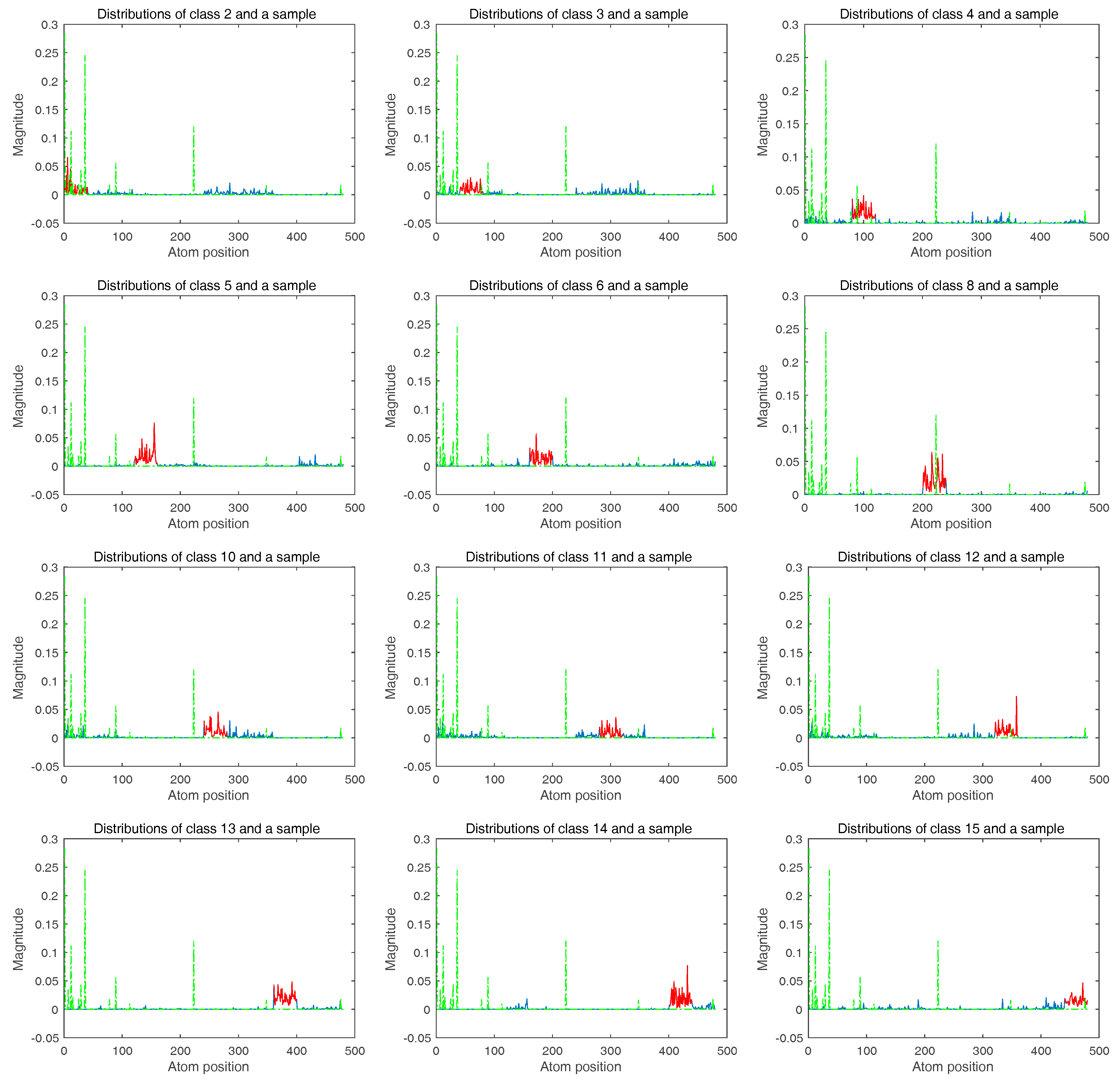
It is generally agreed that SR coefficients follow a class-dependent distribution, which means the nonzero entries of the recovered coefficients from the same class tend to locate at a specific sub-dictionary, and the magnitudes of the coefficients in accordance with the true class are larger than the others. Therefore, in [27], the class-dependent sparse representation classifier (cdSRC) was proposed for HSI classification, where SRC combines K-NN in a class-wise manner to exploit both correlation and Euclidean distance between test and training samples, and the classification performance is increased. Furthermore, K-NN Euclidean distance and the spatial neighboring information of test pixels are introduced into the CR classifiers. In [28], a nonlocal joint CR with a locally-adaptive dictionary is developed. In [29], spatially multiscale adaptive sparse representation in a pixel-wise manner is utilized to construct a structural dictionary and outperforms its counterparts. However, the spatially multiscale pixel-wise operation requires extra computational cost. In [30], the spatial filter banks were included to enhance the logistic classifier with group-Lasso regularization. In addition, kernelized CRC (KCRC) is investigated for HSI classification in [31], and accumulated assignment using a sparse code histogram is discussed in [32].

More recently, some sparse representation-based nearest neighbors (SRNN) and elastic net representation-based classification (ENRC) for HSI are also reported. In [33], three sparse representation-based NN classifiers, i.e., SRNN, local SRNN and spatially-joint SRNN, were proposed to achieve much higher classification accuracy than the traditional Euclidean distance and representation residual. In [34], the proposed ENRC classification method produces more robust weight coefficients via adopting ${\ell }_1$ and ${\ell }_2$ penalties in the objective function, thereby turning out to be more discriminative than the original SRC and CRC. In a word, such representation-based methods are designed to improve the stability of the sparse codes and their discriminability by modeling the spectral variations or collaboratively coding multiple samples.

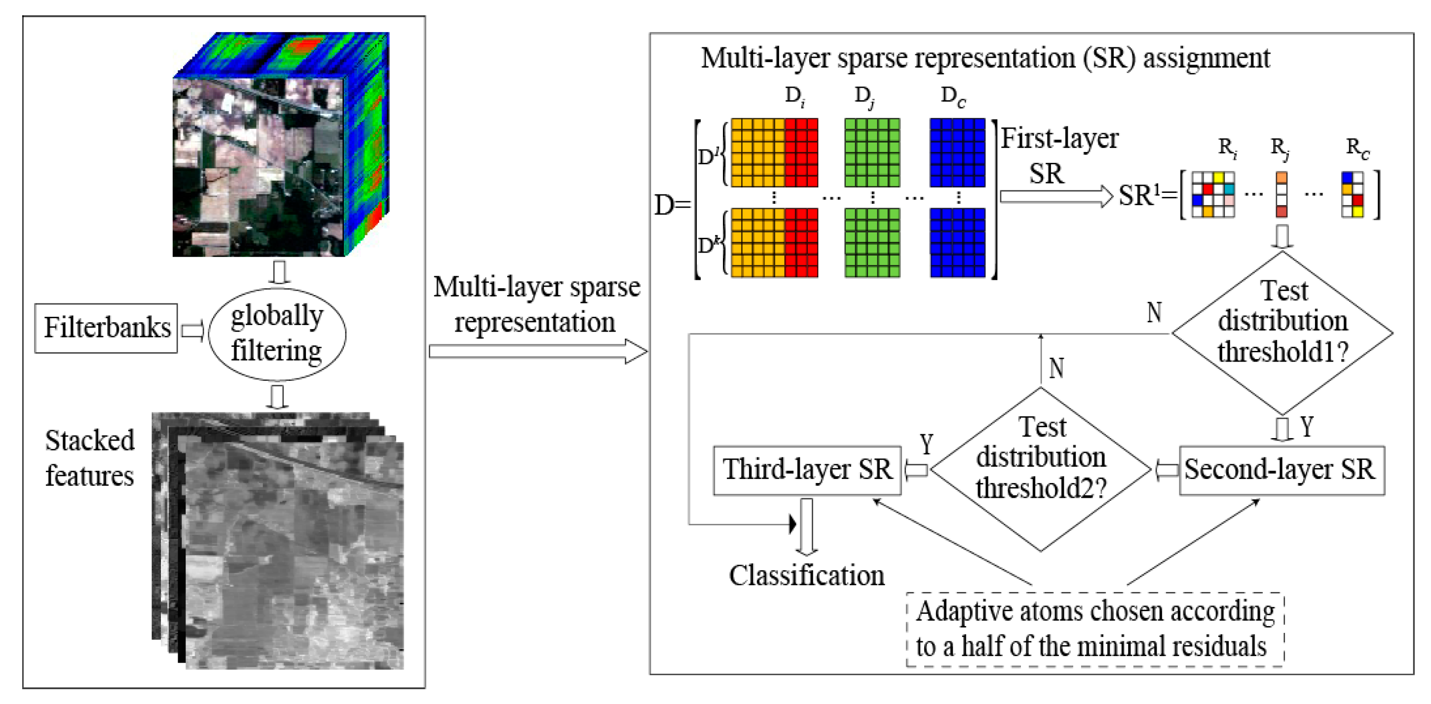
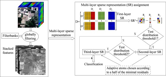
Although the aforementioned representation-based classification methods perform well to some extent, all of them reconstruct sparse coefficients in a single layer and still need to be further exploited in terms of how to estimate the “true” reconstruction coefficients for the test sample. In fact, a multi-layer sparse representation-based (mlSR) assignment framework is preferred to necessarily stabilize the sparse codes for representation-based classification. In this paper, we propose to investigate a multi-layer spatial-spectral SR assignment framework under the structural dictionary for HSI classification, which effectively combines the ideas of a multi-layer SR assignment framework with adaptive dictionary assembling and adaptive regularization parameter selection. Specifically, three SR algorithms, multi-layer SRC (mlSRC), multi-layer CRC (mlCRC) and multi-layer ENRC (mlENRC) are developed. The proposed mlSR assignment framework enforces the selected bases (dictionary atoms) into as few categories as possible, and the estimated reconstruction coefficients are refined thereby, which boosts the accurate discrimination of the model. This is one feature of our method. Another one is that the proposed mlSR assignment framework exploits the intrinsic class-dependent distribution, which is utilized to stabilize test distribution estimation across multiple classes and lead to a selective multi-layer representation-based classification framework. Moreover, we consider the construction of the structural dictionary, that is, a dictionary consisting of spectral and spatial features via the utilization of a group of globally-spatial filter banks is first constructed, thus integrating the spatial consistency of the dictionary atoms and allowing drastic savings in computational time. The proposed mlSR assignment framework is not only natural and simple, but also indeed beneficial toward HSI classification. Note that these features compose our major contributions in this work and make the proposed methods unique with regard to previously-proposed approaches in this area (e.g., [29,35,36]). Our mlSR framework is different from [35] in terms of the implementation principle, where the latter can be viewed as a kind of weighted sparse coding, and the classification is done by maximizing the feature probability, but without dictionary assembling; meanwhile, unlike [29,36], which are designed to capture spatial correlations by introducing the neighboring pixels of the test sample for sparse coding and often time consuming, our proposed methods are in essence a multi-layer framework, which involves assembling adaptive dictionaries for test samples. The experimental results demonstrate that classification accuracy can be consistently improved by the proposed mlSR assignment framework.

There are three main contributions in this work. First, a multi-layer spatial-spectral sparse representation (mlSR) framework for HSI classification is proposed. In the proposed framework, three algorithms, multi-layer SR classification (mlSRC), multi-layer collaborative representation classification (mlCRC) and multi-layer elastic net representation-based classification (mlENRC), are developed and achieve stable assignment distributions via the adaptive atoms selection in a multi-layer manner. Second, both the test distribution evaluation-based filtering rule and dictionary assembling based on the classes ranked within the top half of the minimal residuals are developed to convey discriminative information for classification and decrease the computational time. Last, but not least, a structural dictionary consisting of globally-filtered spatial and spectral information is constructed to further boost the classification performance. It is also worth mentioning that our proposed mlSR framework has another nice property that can be easily plugged into any representation-based classification model using different HSI features (e.g., spectral features, spatial features and spatial-spectral features). The proposed approach is evaluated using three real HSI datasets. The experimental results verify the effectiveness of our proposed methods as compared to state-of-the-art algorithms.

The remainder of this paper is organized as follows. Section 2 briefly reviews representation-based techniques for HSI classification. Section 3 presents the proposed mlSR framework and classification approaches in detail. Section 4 evaluates the proposed approaches against various state-of-the-art methods on three real HSI datasets in terms of classification accuracy and computational time. Section 5 includes discussions of our framework and method. Finally, Section 6 concludes the paper.

2. Representation-Based HSI Classification

2.1. Sparse and Collaborative Representations

As a natural way in signal representation, sparse representation (SR) assumes that the input samples of a particular class lie in a low-dimensional subspace spanned by dictionary atoms (training samples) from the same class. A test sample can be represented as a linear combination of training samples from all classes. Formally, in SR-based classification (SRC), for a test sample $y\in R^d$ (d is the number of the features of HSI), the objective of SR according to the ${\ell }_1$-norm is to find sparse coefficient vector ${\alpha }^{(SR)}$ with a given $d\times N$ structural dictionary $D$, so the objective function can be formulated as:

$${\widehat{\alpha }}^{(SR)}=\arg \underset{{\alpha }^{(SR)}}{\min }||y-D{\alpha }^{(SR)}|{|}_2^2+\lambda ||{\alpha }^{(SR)}|{|}_1$$

(1)

where N is the total number of atoms in D. $\left|\right|·|{|}_1$ denotes the ${\ell }_1$-norm. $\lambda$ is the regularization parameter that balances the contribution of the reconstruction error and the sparsity of the reconstruction weights. Once the sparse coefficient ${\widehat{\alpha }}^{(SR)}$ is obtained, the class label of the test sample y can be determined by the minimal residual error between y and the class-dependent sub-dictionary of each class.

$$r_c^{SRC}(y)=||y-D_c{\widehat{\alpha }}_c^{(SR)}|{|}_2,c=1,\mathrm{...},C$$

(2)

where $C$ is the number of classes and ${\widehat{\alpha }}_c^{(SR)}$ represents the coefficients in ${\widehat{\alpha }}^{(SR)}$ belonging to the c-th class. The class label is given by SRC:

$$clas{s}^{SRC}(y)=\arg {\min }_{c=1,\mathrm{...},C}{r}_c^{SRC}(y)$$

(3)

Different from SRC, in collaborative representation-based classification (CRC), a test sample is represented collaboratively over all of the training samples, and the objective is to find the weight vector ${\widehat{\alpha }}^{(CR)}$, which can be expressed as:

$${\widehat{\alpha }}^{(CR)}=\arg \underset{{\alpha }^{(CR)}}{\min }||y-D{\alpha }^{(CR)}|{|}_2^2+\lambda ||{\alpha }^{(CR)}|{|}_2^2$$

(4)

with $\lambda$ being the regularization parameter. By taking derivative with regard to ${\alpha }^{(CR)}$ in Equation (4), ${\widehat{\alpha }}^{(CR)}$ can be solved as:

$${\widehat{\alpha }}^{(CR)}={(D^{T}D+\lambda \mathrm{I})}^{-1}{D}^{\mathrm{T}}y$$

(5)

Then, the class label assignment by CRC is determined according to the minimum residual $r_c^{CRC}(y)$. Obviously, CRC is more computationally efficient than SRC due to the closed-form solution as in Equation (5).

2.2. Elastic Net

The reconstruction weights play an important role in representation-based classification. Thus, many representation-based methods aim to obtain the weight vector based on some reasonable constraint. For instance, in SRC, training samples are projected onto a subspace, and only a few dictionary atoms (sparsity) are allowed to be selected to form sparse representation, which becomes inaccurate when dictionary atoms are less related and small; while in CRC, many dictionary atoms collaborate on the representation of a test sample and contribute to the reconstruction (collaboratively). Nevertheless, the non-sparse vector of CRC might distribute across multiple classes, and its discriminant ability is limited. Recent literature [34] has pointed out that the classification improvement in some cases is brought by SR, while in other cases, the gain is brought by CR. In order to avoid the aforementioned problem, the elastic net model was recently presented and resulted in robust coefficients via a convex combination of SR and CR [37]. The objective function of elastic net representation-based (ENR) classification (ENRC) is defined as:

$${\widehat{\alpha }}^{(EN)}=\arg \underset{{\alpha }^{(EN)}}{\min }||y-D{\alpha }^{(EN)}|{|}_2^2+{\lambda }_1||{\alpha }^{(EN)}|{|}_1+{\lambda }_2||{\alpha }^{(EN)}|{|}_2^2$$

(6)

where the nonnegative parameters ${\lambda }_1$ and ${\lambda }_2$ are used to control the contributions of the sparsity constraint and self-similarity constraint, respectively. The first constraint encourages sparsity in the reconstruction weights, and the second constraint enforces similarity in their collaborations. The ${\ell }_1$-norm and ${\ell }_2$-norm regularization terms are utilized together in the objective function to overcome the limitation of SR-based and CR-based methods, respectively. Therefore, the highly correlated samples are guaranteed to be selected, and the intrinsic sparsity is enforced by the ENRC. After obtaining ${\alpha }^{(EN)}$, the class label of the test sample y is then determined according to the minimum residual $r_c^{ENRC}(y)$, similar to Equation (2). As a result, the ENRC may offer a correct label assignment even when both SRC and CRC give wrong labels.

3. Proposed Classification Framework

3.1. Motivation for the Proposed Approach

It is well known that the HSI data are characterized with high correlation with each other and spatial variation of spectral signatures, which makes single-layer SR/CR/ENR-based classification methods challenging. This is because the recovered coefficients under such scenarios potentially are instable. The instability implies that the nonzero entries of the recovered coefficients might distribute across multiple classes, thus deteriorating the discriminability. In other words, multi-layer sparse representation is preferred. Intuitively, the more classes associated with the top several minimal residuals can be kept for dictionary assembling, the more accurate the class label of the test sample expected to be assigned. Therefore, we can enforce dictionary assembling into few categories in a multi-layer manner, and the regularization parameter for each test sample is adaptively chosen by cross-validation again. To better understand the working mechanism of the proposed method, we randomly take four test samples located at ((21, 6), (25, 7), (18, 13), (18, 6)) in the Indian Pines for example and calculate respective recovered coefficients using SRC, CRC and ENRC for at most three layers. The sparse coefficients and corresponding residuals of each test sample under various norms are shown in Figure 1. From this figure, one can easily notice that, although all the four test samples belong to Class 2, the single-layer hard assignments of SRC, CRC and ENRC for the considered test samples are inaccurate because the residual error computed from Class 2 is higher than that from some other classes. However, the samples with obviously the wrong class label assigned by the single-layer SRC, CRC and ENRC are enforced to carry out the second-layer SR, even the third-layer SR, respectively, and then assigned the correct class label, which clearly denotes the effectiveness and superiority of this proposed mlSR assignment framework. It should be noted that the structural dictionary consisting of globally-spatial and spectral information is combined to further boost the classification performance.

3.2. Test Distribution Evaluation

According to the above observation, the recovered coefficients follow a class-dependent overall distribution despite the instability in a single-layer SR, and the nonzero entries of the recovered coefficients from the same class tend to locate at a specific sub-dictionary; and the magnitudes of the coefficients corresponding to the true class are usually larger than the others. Perceptually, a test sample y is correctly assigned the class label because this sample has the largest magnitude of sparse coefficients within the active sub-dictionary. We introduce the following heuristics to find out the obviously misclassified samples, which will be accepted to perform a second-layer SR, and newly-assigned class labels of those samples are updated. Similarly, a third-layer SR can be done in the same way. This is based on the following reasons. First, less test samples that will be accepted to carry out multi-layer SR means less computational time for the proposed method. Second, some obviously correctly-assigned samples are unnecessary to run in the subsequent layers. As a result, the classification accuracy of such a selective multi-layer SR assignment framework is consistently improved. To this end, we first adopt the sparsity concentration index (SCI) [38] as the degree measurement across multiple classes:

$$\mathrm{SCI}(\alpha )=\frac{C·{\max }_i\left|\right|{\delta }_i(\alpha )|{|}_1/|\left|\alpha \right|{|}_1-1}{C-1}$$

(7)

where ${\delta }_i(\alpha )$ indicates the entries associated with i-th class. Obviously, in SR via the ${\ell }_1$-norm, for a test sample y, if SCI(α_y) = 1, y is definitely represented using a unique class, and if SCI(α_y) = 0, the sparse coefficients are spread evenly over all classes. Furthermore, we define the heuristic as follows. Specifically, for a test sample y with its label assigned by the lth (l > 0) layer classification as L_l(y), it is accepted to do a multi-layer SR based on the following condition of being ‘true’.

$${\tau }^l(y)=\{\begin{array}{l}true,\mathrm{SCI}({\alpha }_y)=0\\ false,\mathrm{SCI}({\alpha }_y)=1\\ true,L_l(y)=cand(\mathrm{Position}(\mathrm{Peak}({\alpha }_y))and\mathrm{SCI}({\alpha }_y))\not\subset (\mathrm{X}({\mathrm{D}}_c^l)-{\epsilon }^l)\\ false,otherwise\end{array},c=1,\mathrm{...},C$$

(8)

where Position(Peak(α_y)) denotes the position of maximal peak of sparse coefficients α from test sample y. $\mathrm{X}({\mathrm{D}}_c^l)$ indicates the lth layer class-dependent overall distribution from class c and can be expressed as a triplet <Peak, Position, SCI>. In addition, the slight fluctuation ε^l is introduced possibly due to the bias of sparse coefficients in each layer. Thus in a sense, the proposed filtering rule for a multi-layer classification via the residual and sparse coefficient together can pick the obviously misclassified samples for the next layer SR. Let us take the Indian Pines image for example, as illustrated in Figure 2.

The class-dependent overall distribution (blue curve and red blocks) of sparse coefficients of twelve classes are obtained using all of the labeled samples of the corresponding class, under a structural dictionary with forty training samples per class. Further, the sparse coefficients (green curve) of a test sample is also plotted. As can be seen, class-dependent sparse coefficients and the magnitudes mainly concentrate at some fixed blocks; that is, the nonzero entries of the sparse coefficient and larger magnitudes are in accordance with the true class. Hence, class-dependent overall distributions convey discriminative information and are exploited to find the obviously misclassified samples at the previous layer. With this treatment, the plotted test sample is recognized as a ‘good’ sample, i.e., this sample is partitioned into the same class as the true class (ID: 2), and it is unnecessary to proceed to do a multi-layer classification. For the non-${\ell }_1$-norm SR, we use a similar rule to filter the obviously misclassified samples to run a multi-layer SR. Note that the heuristic rule in Equation (8) has the advantage of both computational efficiency and achieving better classification performance over several state-of-the-art methods.

3.3. mlSR Framework

Motivated by the above observations, we propose a novel multi-layer sparse representation (mlSR) framework to explore the stable assignment distribution. To summarize, the overall outline of the proposed mlSR is shown in Figure 3. As depicted in Figure 3, for each test sample, the method consists of the following main steps: (1) compute the sparse coefficients and residual matrices at the first layer; (2) select the obviously misclassified samples at the first layer to perform the second layer SR according to the top C/2 minimal residuals based on the test distribution evaluation and dictionary assembling, and update the corresponding class label assignments; (3) choose the obviously misclassified samples at the second layer to carry out the third layer SR according to the top C/4 minimal residuals on the basis of the predefined test distribution evaluation, and update the corresponding class labels; (4) output the final class labels.

One of the key ingredients in the proposed mlSR framework is that adaptive selection of the sub-dictionary atoms, that is, the new sub-dictionary that are re-assembled for each test sample based on the test distribution evaluation and the classes ranked within the top half of minimal residuals (i.e., C/2 classes in the second layer, C/4 in the third layer, and so on) and appropriate for representing the test sample. In other words, a subset of the structured dictionary is re-selected for the SR of each test sample, favoring a stable assignment distribution and resulting in better discriminative ability of the proposed approach. In addition, the filtering rule for obviously misclassified samples sieved into the next layer SR is another core part of the proposed method because, on the one hand, the correctly-assigned samples at the first layer are unnecessary to do subsequent layer SR according to Equation (8); on the other hand, the new cross-validation on the parameter searching from the second layer is conducted for each test sample and time costly. Thus, a tradeoff between the number of samples filtered to do a multi-layer SR and classification performance should be made. Furthermore, the proposed mlSR framework is detailed in Algorithm 1.

In the proposed framework, the globally-filtered spatial features, such as the widely-used band ratios from the three first principal components (PCs) of original spectral features, 2D Gabor energy [12] and morphological files [5], are extracted and employed to construct the structural dictionary. Note that different types of global features exploit the local information of each considered pixel and should contribute to the discrimination of dictionary atoms; meanwhile, the globally spatial features are much faster to be extracted. These considered features are reported in

Table 1. Types of features except for spectra via globally filtering in the experiments.

Features	Description
Ds	Original spectral information
Dr	Band ratios from the three first PCs [5]
Dg	2D Gabor energy [12]
Dm	Morphological profiles [5]

. As shown in Table 1, D_{{s, r, g, m}} indicates that different types of features except for spectra are globally extracted via different spatial filter banks.

Algorithm 1. Multi-layer spatial-spectral sparse representation classifier.

Input: Layer l = 1, a structural dictionary Dl with M features and N samples; number of classes C; regularization parameter set ${\lambda }_{all}$, test index set $U^l$, threshold εl and residual rl = $\phi$

Step 1: Calculate lth layer class-dependent overall distribution X(Dl)

Step 2: for each test sample y do

Step 3: Determine the optimal regularization parameter λ, λ2 via five-fold cross-validation searching in ${\lambda }_{all}$ under the dictionary Dl

Step 4: Compute sparse coefficients ${\alpha }^{(SR)}$, ${\alpha }^{(CR)}$, ${\alpha }^{(EN)}$ using Equations (1), (5) and (6), respectively

Step 5: Obtain individual residuals $r_c^{SRC}(y)$, $r_c^{CRC}(y)$, $r_c^{ENRC}(y)$ according to Equation (2), and update respective class label matrices $L_l^{SRC}$, $L_l^{CRC}$, $L_l^{ENRC}$

Step 6: Evaluate test distribution ${\tau }^l(y)$ based on X(Dl)

Step 7: Add y into the (l + 1)th test set Ul+1 if ${\tau }^l(y)$ = true

Step 8: Find newly-selected atoms’ indexes and assemble the sub-dictionary according to the classes ranked within the top half of the minimal residuals

Step 9: l ← l + 1, if l > 2 or Ul = NULL; go to the Step 12

Step 10: Go to the Step 3

Step 11: end for

Step 12: Decide the final class label $clas{s}^{SRC}(y)$, $clas{s}^{CRC}(y)$, $clas{s}^{ENRC}(y)$ according to Equation (3)

Step 13: Output: class(y)

4. Experiments

In this section, in order to demonstrate the superiority of the proposed method in HSI classification, the proposed multi-layer spatial-spectral sparse representation (mlSR) method is compared with various state-of-the-art methods on three benchmark hyperspectral remote sensing images: Indian Pines, University of Pavia and Salinas. Note that the proposed method utilizes a structural dictionary consisting of globally-filtered spatial feature such as 2D Gabor (scale = 2, orient = 8), morphological profiles and spectral feature along all bands. To further validate the effectiveness of the proposed model on exploring the structural consistency in the classification scenarios, we compare the proposed mlSR assignment framework with competitors built on only spectral features. Meanwhile, the number of the layers is set as three in order to balance computational complexity and classification performance. Additionally, we also analyze the influence of several key model parameters.

4.1. Hyperspectral Images and Experiment Setting

Three hyperspectral remote sensing images are utilized for extensive evaluations of the proposed approach in the experiments: Indian Pines image captured by AVIRIS (Airborne Visible/Infrared Imaging Spectrometer), University of Pavia image captured by ROSIS (Reflective Optics System Imaging Spectrometer) and Salinas image collected by AVIRIS sensor.

The Indian Pines image was acquired by the Airborne Visible/Infrared Imaging Spectrometer (AVIRIS) sensor over northwest Indiana’s Indian Pine test site in June 1992 [39]. The image contained 16 classes of different crops at a 20-m spatial resolution with the size of 145 × 145 pixels. After uncalibrated and noisy bands were removed, 200 bands remained. We use the whole scene, and twelve large classes are investigated. The number of training and testing samples is shown in

Table 2. Information classes and the number of labeled samples for four considered image datasets.

Class	Indian Pines Name (# Labeled)	University of Pavia Name (# Labeled)	Salinas Name (# Labeled)
C1	Alfalfa (54)	Asphalt (6631)	Brocoli-green-weeds-1 (2009)
C2	Corn-notill (1434)	Meadows (18,649)	Brocoli-green-weeds-2 (3726)
C3	Corn-min (834)	Gravel (2099)	Fallow (1976)
C4	Corn (234)	Trees (3064)	Fallow-rough-plow (1394)
C5	Grass/pasture (497)	Metal sheets (1345)	Fallow-smooth (2678)
C6	Grass/trees (747)	Bare soil (5029)	Stubble (3959)
C7	Grass/pasture-mowed (26)	Bitumen (1330)	Celery (3579)
C8	Hay-windrowed (489)	Bricks (3682)	Grapes-untrained (11,271)
C9	Oats (20)	Shadow (947)	Soil-vineyard-develop (6203)
C10	Soybeans-notill (968)		Corn-senesced-green-weeds (3278)
C11	Soybeans-min (2468)		Lettuce-romaine-4wk (1068)
C12	Soybeans-clear (614)		Lettuce-romaine-5wk (1927)
C13	Wheat (212)		Lettuce-romaine-6wk (916)
C14	Woods (1294)		Lettuce-romaine-7wk (1070)
C15	Bldg-grass-trees-drives (380)		Vineyard-untrained (7268)
C16	Stone-steel (95)		Vineyard-vertical-trellis (1807)

.

The University of Pavia utilized in the experiments is of an urban area that was taken by the ROSIS-03 optical sensor over the University of Pavia, Italy [40]. The image consists of 115 spectral channels of size 610 × 340 pixels with a spectral range from 0.43 to 0.86 μm with a spatial resolution of 1.3 m. The 12 noisy channels have been removed, and the remaining 103 bands were used for the experiments. The ground survey contains nine classes of interest, and all classes are considered. The number of training and testing samples is summarized in Table 2.

The Salinas image was also collected by the AVIRIS sensor, capturing an area over Salinas Valley, CA, USA, with a spatial resolution of 3.7 m. The image comprises 512 × 217 pixels with 204 bands after 20 water absorption bands are removed. It mainly contains vegetables, bare soils and vineyard fields. The calibrated data are available online (along with detailed ground-truth information) from http://www.ehu.es/ccwintco/index.php/Hyperspectral_Remote_Sensing_Scenes. There are also 16 different classes, and all are utilized; the number of training and testing samples is listed in Table 2.

The parameter settings in our experiments are given as follows.

(1) For training set generation, we first randomly select a subset of labeled samples from the ground truth. Then, we randomly choose some samples from the selected training set to build the dictionary. For all of the considered images, different training rates are employed to examine the classification performance of various algorithms. We randomly select a reduced number of labeled samples ({5, 10, 20, 40, 60, 80, 100, 120} samples per class) for training, and the rest are for testing. The classification results and maps of our approach and other compared methods are generated with 120 training samples per class.

(2) For classification, we report the overall accuracy (OA), average accuracy (AA), class-specific accuracies (%), kappa statistic (κ), standard deviation and computational time (including searching the optimal regularization parameters) derived from averaging the results after conducting ten independent runs with respect to the initial training set.

(3) For performance comparison, some strongly-related SR/CR-based methods, including kernelized SRC (KSRC) and KCRC, attribute profiles-based SRC (APSRC) and CRC (APCRC) and their multi-layer versions (i.e., mlAPSRC, mlAPCRC), have been implemented. As the basic classifiers, SVM and representation-based classification (SRC, CRC) and attribute profiles-based SVM (APSVM) are compared; furthermore, the elastic net representation-based classification (ENRC) method is also compared.

(4) For implementation details, to make the comparisons as meaningful as possible, we use the same experimental settings as [41], and all results are originally reported. For Indian Pines and Salinas image datasets, the attribute profiles (APs) [42] were built using threshold values in the range from 2.5% to 10% with respect to the mean of the individual features, with a step of 2.5% for the standard deviation attribute and thresholds of 200, 500 and 1000 for the area attribute, whereas the APs in the University of Pavia image were built using threshold values in the range from 2.5% to 10% with respect to the mean of the individual features and with a step of 2.5% for the definition of the criteria based on the standard deviation attribute. Values of 100, 200, 500 and 1000 were selected as references for the area attribute. The fluctuation epsilon in Equation (8) is heuristically found and 10% of the class atom position range in our experiments. It should be noted that each sample is normalized to be zero mean, unit standard deviation, and all of the results are reported over ten random partitions of the training and testing sets. All of the implementations were carried out using MATLAB R2015a on a desktop PC equipped with an Intel Core i7 CPU (3.4 GHz) and 32 GB of RAM.

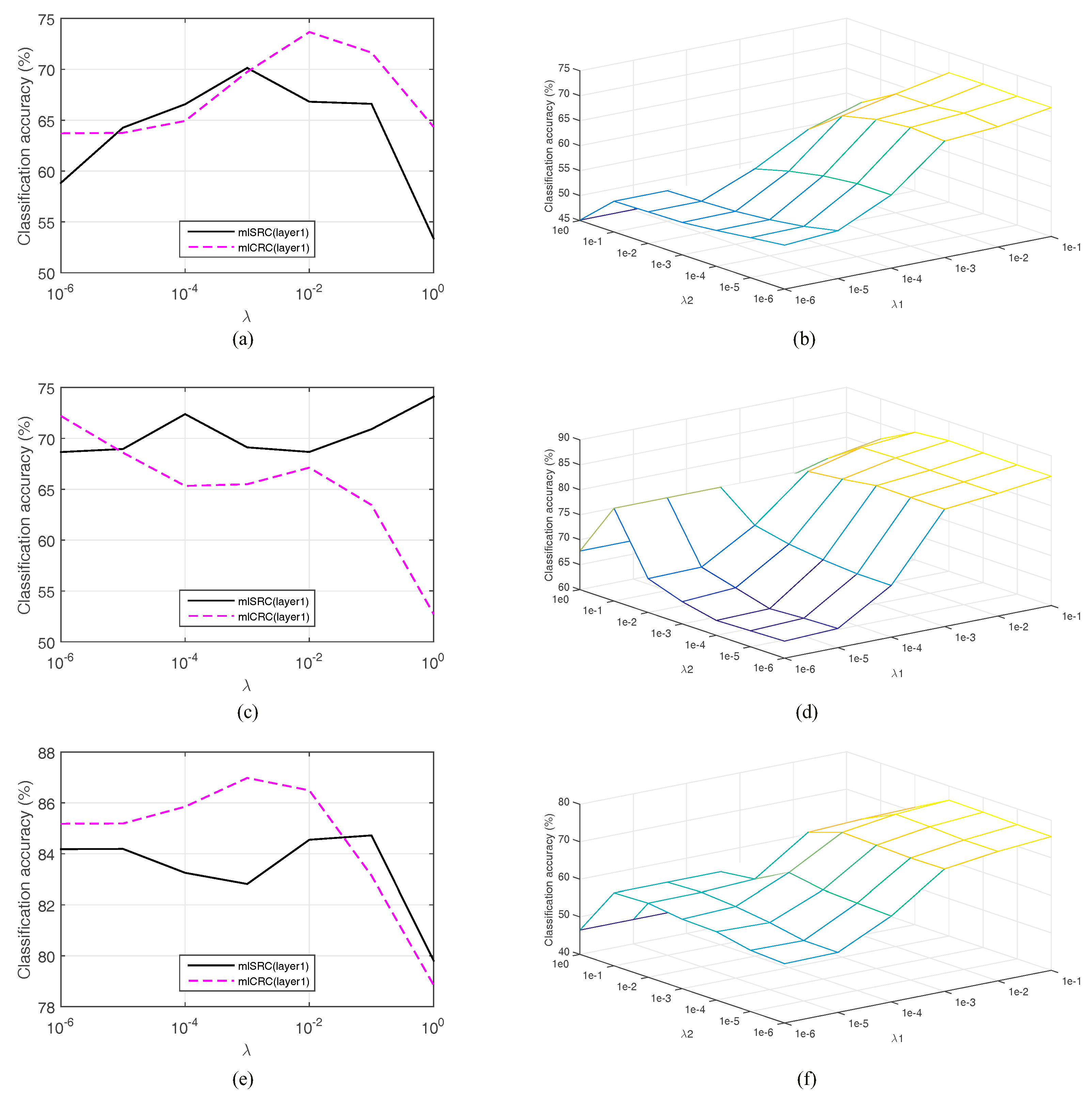
4.2. Model Parameter Tuning

We investigate the parameters of the proposed classification framework. As a regularized parameter, the adjustment of λ is important to the performance of representation-based classifiers. We conduct the five-fold cross-validation test using training data by a linear search in the range of [1 × 10⁻⁶ 1 × 10⁻⁵ 1 × 10⁻⁴ 1 × 10⁻³ 1 × 10⁻² 1 × 10⁻¹ 1] for the regularization parameter in the proposed method. The associated parameters for other considered methods are also done in the same way. We empirically found that best regularization parameters specific to individual methods led to good performance. It can be noted that the regularization parameters from the second layer in the proposed method are sub-dictionary dependent and specific; namely, the five-fold cross-validation from the second layer is done for each test sample, which can achieve higher accuracy, but requires more computational time. For simplicity, Figure 4a–f show the overall classification accuracies of three proposed representation-based classifiers in the first layer versus the regularization parameter λ for the Indian Pines, University of Pavia and Salinas images, respectively. Similarly, the parameter tuning of λ for other investigated methods are also observed. Note that the optimal parameter λ is varied according to different training rates.

4.3. Experiment 1: Results on the Indian Pines Classification

We perform a comparative evaluation of our proposed mlSR approach against several state-of-the-art sparse classification methods mentioned above, as summarized in

Table 3. Overall classification accuracy (%) and standard deviation as a function of the number of training samples per class for the Indian Pines image. KSRC, kernelized SRC; AP, attribute profile.

Algorithm	Training Samples per Class
	5	10	20	40	60	80	100	120
SVM	49.47 ± 3.41	57.99 ± 3.77	66.22 ± 1.55	74.13 ± 1.27	78.11 ± 1.19	80.57 ± 0.97	81.93 ± 1.08	83.52 ± 0.78
SRC	46.56 ± 3.49	53.84 ± 2.85	60.01 ± 1.53	65.90 ± 1.17	68.53 ± 1.28	70.75 ± 1.15	72.44 ± 1.25	73.40 ± 0.63
CRC	46.01 ± 4.80	51.18 ± 3.00	60.63 ± 2.85	66.10 ± 0.84	67.52 ± 1.48	69.33 ± 1.03	69.49 ± 1.44	69.74 ± 1.12
ENRC	47.63 ± 0.20	56.55 ± 0.10	63.72 ± 0.54	67.66 ± 0.25	68.72 ± 3.60	71.54 ± 3.57	73.90 ± 1.56	75.42 ± 0.39
KSRC	47.71 ± 3.57	58.31 ± 3.20	66.68 ± 1.38	73.85 ± 1.59	77.82 ± 1.08	79.76 ± 0.84	81.87 ± 0.63	82.82 ± 0.77
KCRC	49.83 ± 3.72	57.50 ± 3.51	67.41 ± 1.79	75.20 ± 1.02	78.69 ± 0.84	81.06 ± 0.61	82.44 ± 0.98	83.85 ± 0.65
mlSRC	48.77 ± 5.93	65.50 ± 6.73	72.07 ± 8.41	78.44 ± 1.17	79.64 ± 2.62	81.25 ± 2.94	83.07 ± 3.53	84.81 ± 3.91
mlCRC	55.42 ± 1.55	70.02 ± 2.62	76.36 ± 1.08	80.21 ± 7.22	81.16 ± 2.34	83.60 ± 3.05	84.72 ± 3.55	85.19 ± 4.04
mlENRC	56.65 ± 6.27	68.19 ± 6.69	73.04 ± 5.70	80.30 ± 4.50	81.25 ± 4.24	84.53 ± 2.37	85.69 ± 3.49	86.87 ± 4.68
APSVM	62.57 ± 5.69	65.90 ± 3.61	80.78 ± 2.50	84.56 ± 0.62	87.19 ± 0.96	88.65 ± 0.89	90.22 ± 0.44	91.23 ± 0.38
APSRC	58.03 ± 3.37	66.25 ± 3.19	73.89 ± 2.26	78.65 ± 1.31	81.32 ± 1.58	83.27 ± 1.61	84.48 ± 0.84	85.62 ± 0.62
APCRC	56.83 ± 0.72	64.55 ± 1.93	68.75 ± 1.97	71.21 ± 1.22	71.93 ± 0.92	71.87 ± 0.54	72.28 ± 0.74	73.07 ± 1.70
mlAPSRC	66.10 ± 1.89	73.66 ± 3.87	81.37 ± 2.15	85.55 ± 0.75	87.97 ± 0.54	89.32 ± 0.88	89.34 ± 0.72	90.21 ± 0.83
mlAPCRC	64.62 ± 2.01	74.98 ± 2.67	81.29 ± 1.21	83.90 ± 0.86	84.76 ± 1.12	85.82 ± 0.57	86.48 ± 0.58	86.59 ± 0.88

and

Table 4. Class-specific accuracy (%), overall (OA), average (AA), kappa (κ), as well as computational time in seconds with 120 training samples per class for the Indian Pines image.

Class	SVM	SRC	CRC	ENRC	KSRC	KCRC	APSRC	APCRC	mlSRC	mlCRC	mlENRC
2	82.21	63.90	64.03	74.74	77.32	80.11	81.48	41.78	84.56	84.56	81.64
3	80.87	63.05	47.56	63.22	79.12	78.66	80.52	70.45	79.58	78.65	86.52
4	94.56	90.26	87.02	93.28	96.49	96.05	93.28	98.25	95.45	99.35	96.91
5	96.34	92.33	91.62	91.69	95.7	95.78	87.91	85.68	95.20	95.20	91.68
6	95.34	95.42	93.62	96.45	96.24	96.75	66.15	58.53	98.05	99.70	97.60
8	99.19	99.59	99.89	100.0	99.54	99.40	99.23	99.19	100.0	100.0	99.78
10	87.49	77.84	77.28	77.88	88.75	88.79	91.71	85.38	90.43	91.55	90.95
11	70.32	54.64	47.77	51.39	69.14	71.33	87.25	82.96	66.79	66.79	74.05
12	89.37	83.18	84.13	88.91	88.83	90.43	75.49	66.19	89.89	94.19	87.63
13	99.35	99.78	99.02	100.0	99.89	99.57	99.11	100.0	100.0	100.0	100.0
14	89.58	88.13	87.44	92.04	91.82	91.02	93.97	73.68	96.38	95.39	98.01
15	85.42	85.23	75.85	86.43	86.19	87.85	82.86	78.46	93.33	94.67	89.12
OA	83.52	73.40	69.74	75.42	82.82	83.85	85.62	73.07	84.81	85.19	86.87
AA	89.17	82.78	79.60	84.67	89.09	89.65	89.79	83.46	90.81	91.67	91.16
κ	0.819	0.715	0.678	0.736	0.812	0.822	0.839	0.707	0.834	0.838	0.856
Time (s)	455.6 ± 0.2	930.4 ± 1.3	903.7 ± 1.1	950.2 ± 0.9	2.7 × 103 ± 0.7	520.6 ± 1.0	941 ± 0.7	962 ± 0.6	3.7 × 103 ± 0.9	3.1 × 103 ± 0.8	4.0 × 103 ± 0.5

. Based on the results in Table 3, one can easily see that the classification performances of the proposed mlSRC, mlCRC and mlENRC approaches considerably and consistently outperform those of the other baseline algorithms (except APSVM and mlAPSRC) over a range of training samples. Table 4 reports the average OA, AA, class-specific accuracies (%), κ statistic and computational time of ten trials in seconds using one hundred and twenty training samples per class (mlAP-based and APSVM are not presented because of the limited column space). As expected, the third best method, mlENRC, with the obtained OA, κ, and AA of 86.87%, 0.856 and 91.16%, respectively, which outperforms the single-layer baselines (e.g., SRC, CRC, ENRC and kernelized versions) and SVM, and the increases of OA, κ, and AA range from 3.02% to 17.13%, 0.034 to 0.178 and 1.51% to 11.56%, respectively. The top two best methods are APSVM (91.23% at 120 training samples) and mlAPSRC (90.21% at the same training ratio) respectively, and the reason is that the attribute profiles provide better discriminative features than the globally-filtered features. To our best knowledge, this result is very competitive on this dataset, which indicates the effectiveness of the proposed mlSR framework.

As can be seen from Table 4, SVM is the fastest, and our proposed mlSRC, mlCRC and mlENRC methods require a larger computational effort, but also achieve better classification accuracy than all competitors. Nevertheless, a fusion strategy using multiple parameters instead of cross-validation for regularization parameter selection at consequent layers can be utilized to reduce the computational time. 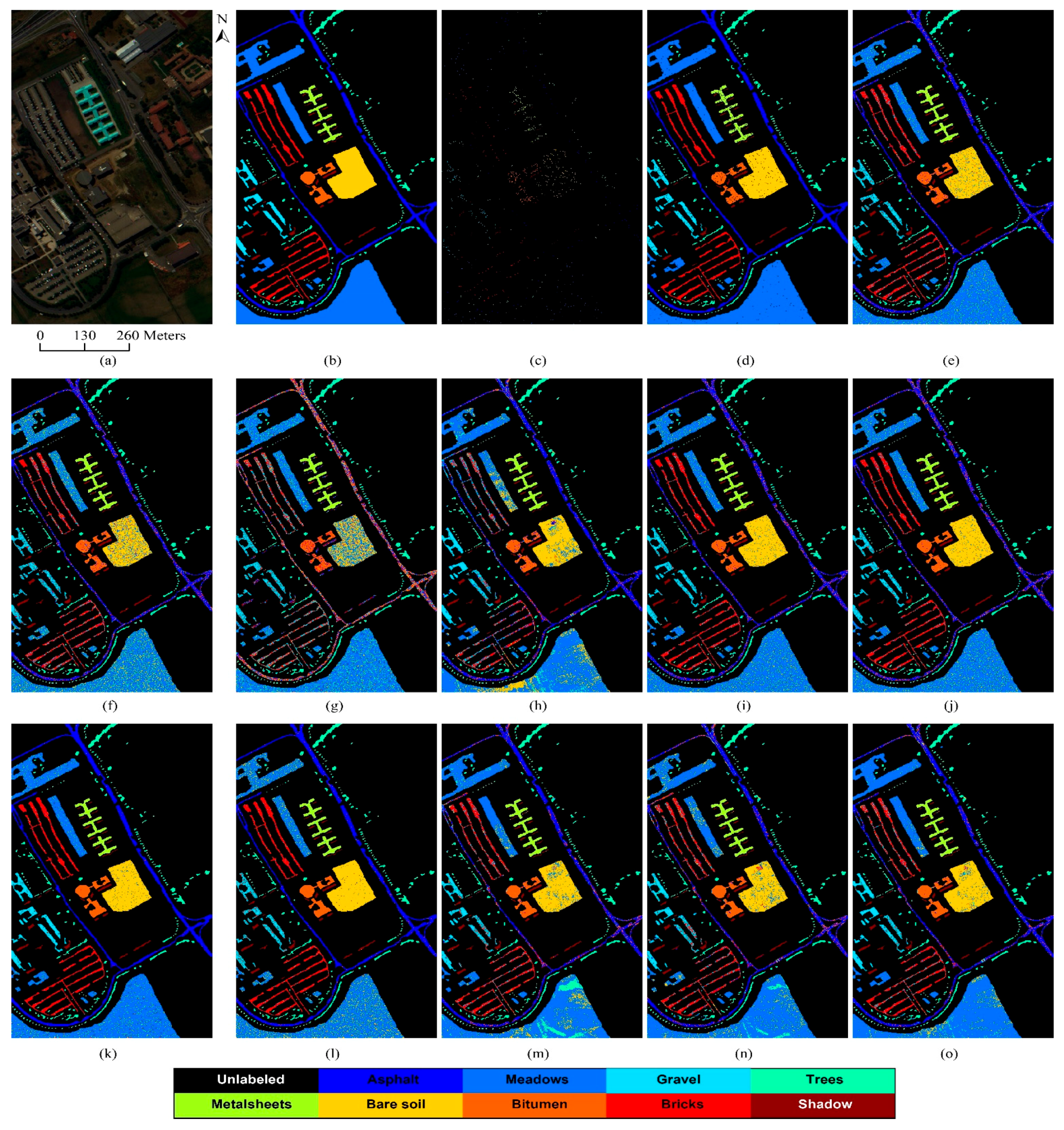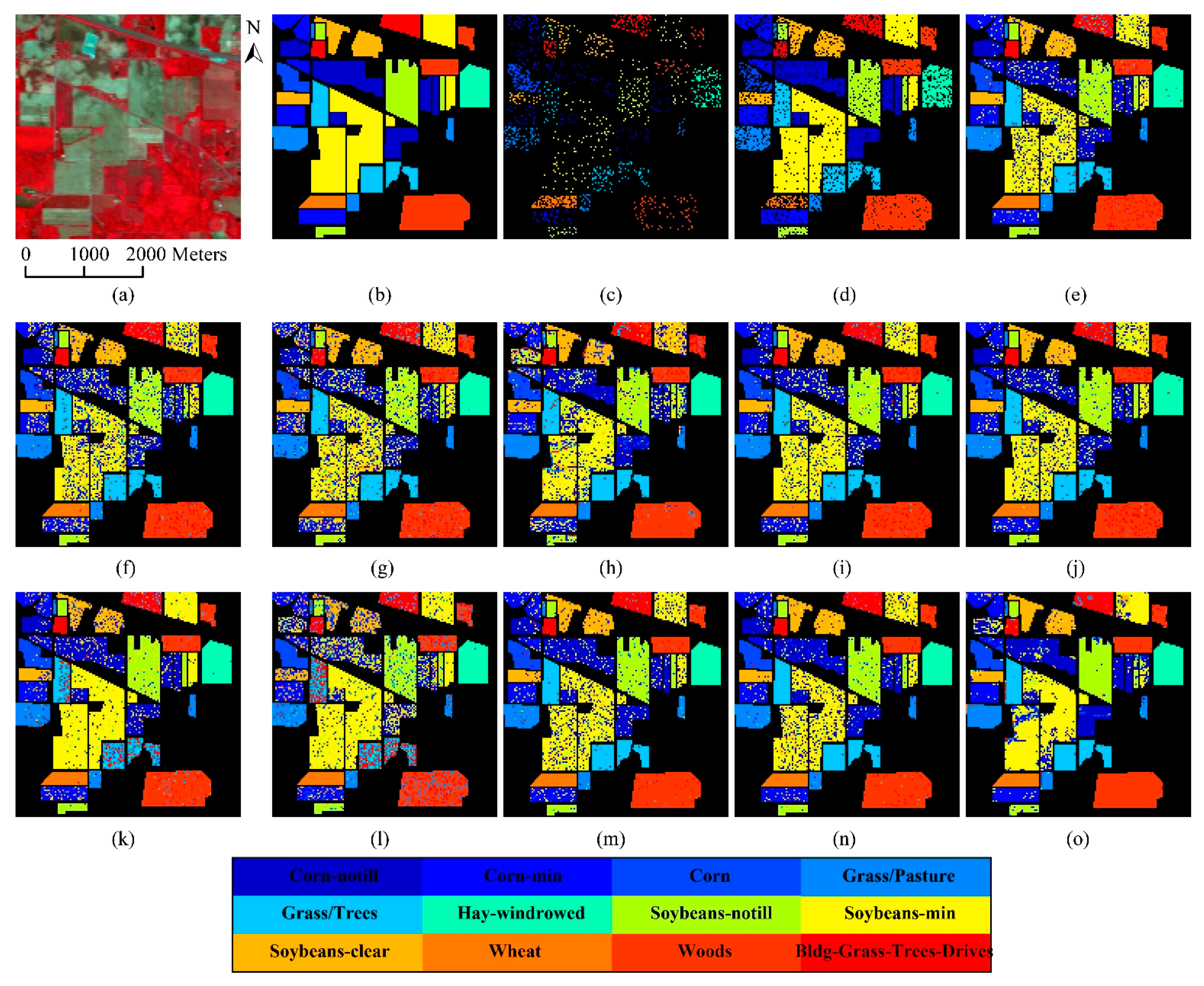The classification maps of the Indian Pines generated using the proposed methods and baseline algorithms are shown in Figure 5 to test the generalization capability of these methods. It is shown in Figure 5 that the three proposed mlSRC, mlCRC and mlENRC methods result in more accurate and “smoother” classification maps (with reduced salt-and-pepper classification noise) compared with traditional SRC/CRC, even kernelized SRC/CRC and SVM, which further validates the effectiveness and superiority of the proposed mlSR assignment framework for HSI classification. The results also show that the single-layer SRC, CRC and ENRC always produce inferior performances on this test set, most likely in part due to the instability of the single-layer SR. Our analysis also shows that the KSRC and KCRC have a comparable performance compared with SVM, mlENRC and mlAPCRC, as well.

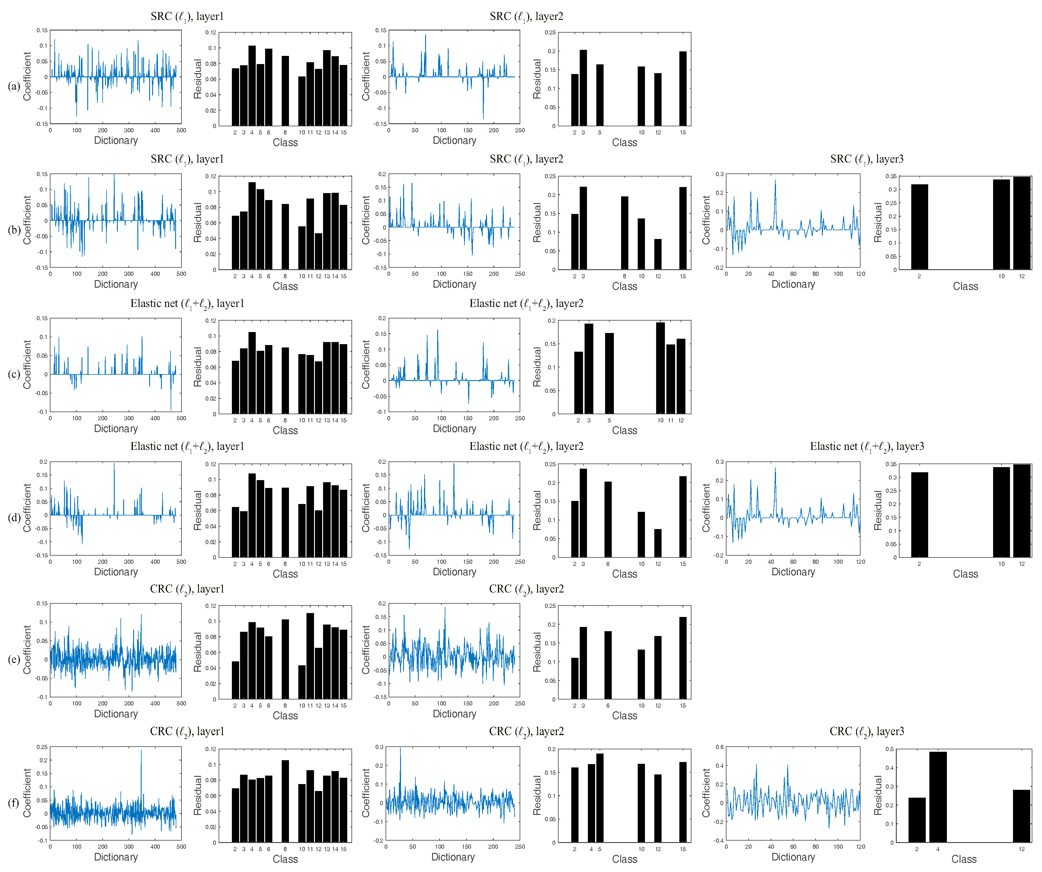
The results in this experiment show that the proposed multi-layer assignment framework is effective to boost classification performance with an improved accuracy of about 3% to 14% via a multi-layer SR. The underlying mechanism of our methods accords with the observation that the sparse coefficients obtained from the second layer lead to a total correct label assignment, where the classes ranked within the top half of the minimal residuals are utilized to do dictionary assembling for each test sample. As a result, the classification performance is guaranteed to increase, which clearly denotes the effectiveness and superiority of the proposed mlSR assignment framework.

4.4. Experiment 2: Results on the University of Pavia Classification

The classification results of the proposed methods and baseline algorithms for the University of Pavia are summarized in

Table 5. Overall classification accuracy (%) and standard deviation as a function of the number of training samples per class for the University of Pavia image.

Algorithm	Training Samples per Class
	5	10	20	40	60	80	100	120
SVM	62.87 ± 8.69	67.09 ± 3.80	76.48 ± 4.42	82.37 ± 2.14	85.81 ± 1.24	86.80 ± 0.87	88.34 ± 0.76	88.57 ± 0.67
SRC	59.20 ± 4.09	64.80 ± 4.13	69.11 ± 1.97	72.75 ± 1.96	76.64 ± 1.14	78.27 ± 1.07	79.17 ± 0.99	79.64 ± 1.09
CRC	52.54 ± 6.74	61.00 ± 3.78	64.13 ± 2.00	64.99 ± 2.31	66.88 ± 2.33	67.59 ± 1.29	67.91 ± 1.08	68.39 ± 1.28
ENRC	61.90 ± 5.50	65.89 ± 3.79	72.97 ± 3.59	76.41 ± 3.79	78.65 ± 3.26	80.29 ± 3.82	81.01 ± 3.96	82.08 ± 2.99
KSRC	61.08 ± 6.44	68.87 ± 4.01	77.85 ± 2.46	82.83 ± 1.81	85.27 ± 1.18	87.55 ± 0.70	88.25 ± 0.83	88.92 ± 0.63
KCRC	64.00 ± 4.58	69.53 ± 4.06	76.80 ± 2.16	81.44 ± 1.97	85.59 ± 1.50	86.32 ± 1.02	87.95 ± 0.55	88.56 ± 0.55
mlSRC	61.78 ± 2.11	68.68 ± 9.44	76.84 ± 9.63	81.76 ± 7.41	85.94 ± 6.18	86.84 ± 4.78	87.64 ± 1.92	88.67 ± 1.55
mlCRC	65.44 ± 3.48	69.72 ± 5.01	77.65 ± 2.57	82.68 ± 0.84	85.82 ± 2.05	87.65 ± 3.59	88.51 ± 1.71	89.65 ± 4.02
mlENRC	61.91 ± 3.09	68.97 ± 4.10	77.93 ± 1.51	82.85 ± 1.00	86.11 ± 5.39	87.79 ± 3.94	88.45 ± 2.54	90.32 ± 1.26
APSVM	63.80 ± 9.43	79.43 ± 2.10	86.60 ± 0.46	89.55 ± 1.62	92.09 ± 0.35	93.08 ± 0.05	94.66 ± 0.38	95.08 ± 0.06
APSRC	74.08 ± 3.55	82.22 ± 3.63	88.89 ± 1.97	89.87 ± 1.41	93.78 ± 0.85	94.20 ± 0.51	94.50 ± 0.49	95.29 ± 0.32
APCRC	72.53 ± 4.16	85.27 ± 1.83	88.32 ± 2.18	88.43 ± 0.81	90.13 ± 0.98	90.27 ± 0.51	91.14 ± 0.17	92.22 ± 1.48
mlAPSRC	82.06 ± 2.99	88.40 ± 2.71	92.64 ± 1.76	93.68 ± 1.27	96.37 ± 0.60	95.89 ± 0.36	96.13 ± 0.42	96.45 ± 0.38
mlAPCRC	84.35 ± 2.39	90.62 ± 2.32	92.08 ± 1.94	93.36 ± 0.97	94.19 ± 0.49	94.49 ± 0.44	94.61 ± 0.74	95.39 ± 0.41

and

Table 6. Class-specific accuracy (%), overall (OA), average (AA), kappa (κ), as well as computational time in seconds with 120 training samples per class for the University of Pavia image.

Class	SVM	SRC	CRC	ENRC	KSRC	KCRC	APSRC	APCRC	mlSRC	mlCRC	mlENRC
1	83.14	76.53	24.52	75.66	79.57	76.89	98.84	97.73	81.91	80.19	82.53
2	88.58	77.50	83.23	82.91	90.21	90.04	92.62	86.88	93.08	92.73	93.50
3	83.23	79.61	85.26	71.55	85.47	86.20	96.73	92.30	88.25	85.96	90.65
4	95.75	95.33	95.37	94.80	96.38	96.20	99.66	97.44	95.11	97.98	95.99
5	99.61	99.79	99.98	99.59	99.52	99.75	99.68	99.52	99.92	99.92	99.92
6	89.11	82.66	53.96	80.77	91.39	91.93	96.42	98.34	89.70	83.04	90.73
7	93.98	88.69	86.64	87.11	95.06	95.52	99.76	99.67	94.88	93.18	93.74
8	83.81	64.91	48.64	74.96	83.39	83.63	92.39	90.12	74.68	76.88	76.10
9	99.94	98.80	42.04	98.91	99.99	99.99	100.0	99.88	98.35	97.79	98.94
OA	88.34	79.64	68.39	82.08	88.92	88.56	95.29	92.22	89.65	88.67	90.32
AA	90.79	84.87	68.85	85.14	91.22	91.13	96.37	93.74	90.65	89.74	91.34
κ	0.855	0.759	0.626	0.783	0.861	0.857	0.940	0.903	0.870	0.858	0.877
Time (s)	420.6 ± 1.1	5.4 × 103 ± 0.4	5.5 × 103 ± 0.8	6.0 × 103 ± 0.7	4.7 × 103 ± 0.6	820.4 ± 0.3	3.7 × 103 ± 1.2	3.8 × 103 ± 0.7	7.4 × 103 ± 1.2	6.5 × 103 ± 0.5	7.8 × 103 ± 0.6

. We compare the classification accuracies of our approaches with traditional SRC and CRC, kernelized SRC and CRC and SVM on this dataset. As in the Indian Pines experiments, our proposed mlSRC, mlCRC and mlENRC methods yield higher classification accuracies than any other baseline algorithms. Observing Table 5, we can find that three proposed mlSRC, mlCRC and mlENRC approaches are consistently better than all baseline methods (except AP-based and mlAP-based) from a small number of training samples (five and ten per class) to a larger one (one hundred and twenty per class). Specifically, as provided in Table 6 (mlAP-based and APSVM are not presented due to the limited column space), the OA, κ and AA for our best approach, mlENRC, can be improved from 1.4% to 21.93%, 0.016 to 0.251 and 0.12% to 22.49%, respectively. More specifically, the increases for mlENRC in OA, κ and AA are about 1.4%, 0.016% and 0.12% than that of the fourth best method, KSRC, respectively. Interestingly, the mlAP-based methods (i.e., mlAPSRC and mlAPCRC) achieve better accuracies than their counterparts (that is, APSRC and APCRC), respectively. This can be due to the better stability of proposed mlSR assignment framework. Moreover, we observe that our proposed methods require the largest time, mainly due to the cross-validation again from the second layer, but the classification performance is improved in spite of relatively slight improvements. In addition, CRC and KCRC are relatively lower than SRC and KSRC. For this dataset, small spatial homogeneity in this image might cause the training samples from other classes also to participate in the linear representation of the test samples, which leads to some misclassification. Visualization of the classification map using 120 training samples per class is shown in Figure 6. The effectiveness of classification accuracies can be further confirmed by carefully visually checking the classification maps. The obvious misclassification among the class of asphalt and the class of shadow by CRC illustrates the inadequacy of the single-layer SR, which is greatly alleviated in Figure 5m–o, and the best result is achieved in Figure 5o. Therefore, the proposed mlSR framework in the classifiers helps in the discrimination of different types of land cover classes.

A similar phenomena can be observed that the multi-layer assignment framework achieves improvements of about 1.2% to 14% to a great extent. The highest accuracy is achieved by mlAPSRC in all training ratios (the second best method is mlAPCRC), which may be associated with the fact that the highly related samples after AP-based processing are chosen to produce a more discriminative power of SRC. Another interesting case is found that AP/mlAP-based methods are always better than non-AP-based ones.

4.5. Experiment 3: Results on the Salinas Classification

To validate the performance of the proposed mlSR, mlCRC and mlENRC with both under-complete and over-complete dictionaries, we have tested over a wide range of numbers of training samples, varying from five samples per class to 120 samples per class and the classification results for this dataset are shown in

Table 7. Overall classification accuracy (%) and standard deviation as a function of the number of training samples per class for the Salinas image.

Algorithm	Training Samples per Class
	5	10	20	40	60	80	100	120
SVM	80.46 ± 1.28	84.24 ± 2.66	86.32 ± 1.29	88.42 ± 1.30	89.64 ± 0.94	90.47 ± 0.68	90.82 ± 0.68	90.92 ± 0.52
SRC	80.12 ± 2.01	82.74 ± 1.58	83.84 ± 1.61	86.21 ± 0.64	86.50 ± 0.73	87.04 ± 0.47	87.50 ± 0.48	88.11 ± 0.54
CRC	76.10 ± 2.27	79.33 ± 1.75	83.45 ± 1.41	85.72 ± 0.90	86.21 ± 0.71	86.89 ± 0.55	87.28 ± 0.51	87.33 ± 0.35
ENRC	79.35 ± 2.79	83.50 ± 1.55	84.51 ± 1.42	86.57 ± 1.49	86.89 ± 1.28	87.78 ± 1.61	87.92 ± 1.51	88.70 ± 1.59
KSRC	81.16 ± 2.45	83.67 ± 2.14	85.11 ± 1.39	85.20 ± 1.12	85.51 ± 0.89	85.65 ± 2.25	86.67 ± 2.61	86.84 ± 2.06
KCRC	81.47 ± 1.66	85.79 ± 1.83	87.40 ± 1.51	89.20 ± 1.01	90.23 ± 0.88	90.74 ± 0.72	90.65 ± 1.00	91.40 ± 0.40
mlSRC	81.54 ± 2.78	86.37 ± 4.03	87.98 ± 1.87	89.42 ± 1.62	90.65 ± 2.17	91.09 ± 2.29	91.28 ± 1.92	91.57 ± 1.43
mlCRC	83.33 ± 1.55	86.84 ± 1.15	88.58 ± 0.56	90.35 ± 1.75	91.43 ± 2.61	91.87 ± 2.71	92.22 ± 2.50	93.05 ± 1.57
mlENRC	84.21 ± 2.77	87.31 ± 2.85	89.22 ± 1.57	89.79 ± 1.58	91.59 ± 1.67	92.03 ± 1.92	92.37 ± 1.30	93.75 ± 1.52
APSVM	82.88 ± 2.18	88.76 ± 1.46	93.81 ± 0.40	93.57 ± 0.74	94.75 ± 0.37	95.55 ± 0.26	96.61 ± 0.55	97.01 ± 0.15
APSRC	80.97 ± 2.09	86.30 ± 2.19	89.80 ± 1.06	91.70 ± 0.72	92.11 ± 0.83	93.25 ± 0.81	94.31 ± 0.28	94.54 ± 0.38
APCRC	80.35 ± 1.27	83.71 ± 4.19	87.42 ± 1.36	89.16 ± 0.99	90.28 ± 0.79	90.77 ± 0.30	91.47 ± 0.39	91.76 ± 0.40
mlAPSRC	87.23 ± 3.53	89.98 ± 2.81	93.92 ± 0.94	94.72 ± 0.72	95.54 ± 1.49	96.11 ± 0.88	96.31 ± 0.32	96.70 ± 0.20
mlAPCRC	89.61 ± 1.71	93.90 ± 1.10	95.26 ± 0.81	95.49 ± 0.49	96.50 ± 0.88	97.04 ± 0.20	97.32 ± 0.34	97.67 ± 0.19

and

Table 8. Class-specific accuracy (%), overall (OA), average (AA), kappa (κ), as well as computational time in seconds with 120 training samples per class for the Salinas image.

Class	SVM	SRC	CRC	ENRC	KSRC	KCRC	APSRC	APCRC	mlSRC	mlCRC	mlENRC
1	99.49	99.83	99.2	99.58	95.67	99.72	98.48	98.57	99.95	100	100
2	99.68	98.36	99.73	99.42	99.12	99.84	99.78	99.67	99.95	99.92	99.92
3	99.59	91.42	98.46	98.81	97.93	99.81	99.20	93.32	97.09	99.43	99.28
4	99.51	98.55	94.24	99.14	98.99	99.55	100.0	99.37	99.56	99.63	99.70
5	98.48	98.54	98.12	98.63	96.87	99.04	99.22	98.83	98.83	99.05	98.26
6	99.81	99.45	99.96	99.79	99.40	99.8	99.84	99.61	99.92	99.95	99.92
7	99.5	99.06	99.76	99.07	99.07	99.66	99.31	98.29	99.63	99.52	99.58
8	78.42	74.12	79.22	71.90	68.70	79.73	95.58	89.81	81.46	83.02	83.30
9	99.33	98.81	99.97	98.90	96.84	99.49	99.13	99.00	99.79	99.97	100
10	94.27	93.59	90.41	93.73	91.12	95.49	97.67	92.75	94.17	97.13	94.60
11	98.67	94.78	96.22	99.26	89.25	98.69	91.74	88.19	97.71	99.81	99.90
12	99.69	97.1	83.81	99.89	96.48	100	100.0	94.96	99.16	99.63	99.58
13	99.46	95.04	86.34	99.75	92.13	99.07	100.0	100.0	98.66	99.66	98.86
14	97.61	92.57	93.55	96.63	90.26	97.91	99.07	96.74	97.90	98.64	97.96
15	72.67	65.62	54.23	67.64	68.00	72.85	71.32	66.96	71.87	77.60	84.14
16	99.01	97.16	97.71	99.53	96.77	99.26	100.0	99.82	98.77	99.55	98.87
OA	90.92	88.11	87.33	88.70	86.84	91.40	94.54	91.76	91.57	93.05	93.75
AA	95.95	93.38	91.93	95.10	92.29	96.24	96.82	94.32	95.90	97.03	97.12
κ	0.901	0.871	0.863	0.878	0.858	0.906	0.940	0.910	0.908	0.924	0.932
Time (s)	487.2 ± 0.3	1.1 × 104 ± 0.4	0.9 × 104 ± 0.2	1.2 × 104 ± 0.6	7.3 × 104 ± 0.1	5.4 × 104 ± 0.4	0.8 × 104 ± 0.1	0.9 × 104 ± 0.1	2.2 × 104 ± 0.2	1.3 × 104 ± 0.6	2.4 × 104 ± 0.4

. Likewise, it can be observed from the results that the proposed mlSRC, mlCRC and mlENRC give a consistently better performance than other non-AP-based algorithms. It is obvious from Table 8 (mlAP-based and APSVM are not presented due to the limited column space) that almost all of the class-specific accuracies are improved and hold for interpreting the consistency of the three proposed mlSRC, mlCRC and mlENRC algorithms. Overall, the OA, κ and AA for this dataset can be improved from 2.35% to 6.91%, 0.026 to 0.074 and 0.88% to 5.19%, respectively. 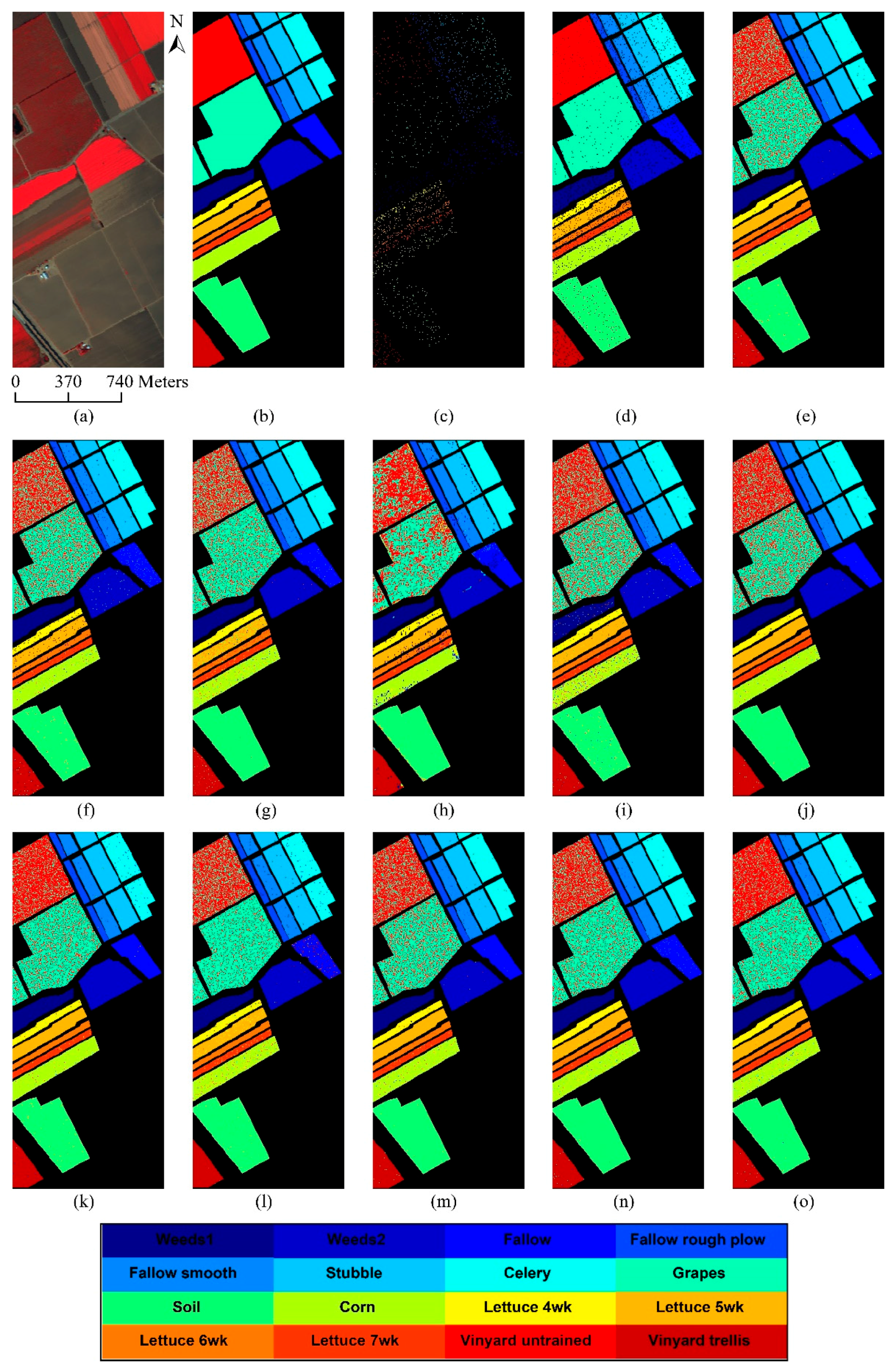Specifically, the increases in OA, κ and AA for the overall best method mlENRC over the fourth best method KCRC are 2.35%, 0.026 and 0.88%, respectively. The best approach is mlAPCRC, which reaches 97.67% when the training ratio is 120 per class. The proposed multi-layer assignment framework and large structure in this HSI may account for this. The classification maps shown in Figure 7 are generated using the proposed algorithms and baselines. Based on the visual inspection in Figure 7, the maps generated from classification using the multi-layer SR framework are less noisy and more accurate than those from using single-layer SR. For example, the classification map of mlENRC (Figure 7o) is more accurate than the map of SVM (Figure 7e). The misclassification of SVM mostly occurred between the class of grapes-untrained and vineyard-untrained. This is explained by the fact that most of the classes in the image represent large structures, and less spatial features could not well capture local structures. Similarly, the proposed methods are computationally intensive during testing. In this case, multiple parameter fusion instead of cross-validation can be employed in order to decrease the computational time. Therefore, the conclusion is that the classification performance of the proposed approaches can be greatly improved via a novel multi-layer SR framework.

As the previous two HSI datasets, the multi-layer assignment framework can obtain an increase of about between 2% and 11% by the introduction of multi-layer SR in the Salinas image, the proposed multi-layer framework accumulates the classification results from different layers, which results in a greater accuracy and is superior to the single-layer hard assignment due to unstable coefficients based on the minimal residual alone. Therefore, the proposed mlSR framework is competent to improve classification performance.

5. Discussion

The design of a proper SR-based classification framework is the first important issue we are facing, as HSI datasets are complex, and the within-class variation and spatial details in complex scenes cannot be well measured by the single-layer SR. In the design of the SR-based model, we propose a multi-layer SR framework to produce discriminative SR for the test samples and achieve stable assignment distributions via the adaptive atoms’ selection in a multi-layer manner, then three proposed approaches, mlSRC, mlCRC and mlENRC, are developed. The proposed mlSRC, mlCRC and mlENRC are based on the same idea, but adopt different sparse optimization criteria. The different criteria bring out the difference among them for HSI classification, and the difference of the three proposed methods is related to the constructing manner of the sparse optimization solver. In order to balance the classification performance and complexity of the framework, the three-layer SR is adopted. Meanwhile, a filtering rule is heuristically exploited to identify the obviously misclassified samples for the next layer SR; moreover, dictionary assembling and new cross-validation on the parameter searching for each test sample are conducted. These enhancements lead to a substantial improvement in performance and saves computational time during testing. Another important observation is that our proposed methods are computationally intensive; this is mainly due to the fact that the optimal regularization parameter for each test sample is searched via cross-validation again from the second layer. Thus, the multiple parameter fusion is expected to be a good alternative to cross-validation in computationally efficiency. Nevertheless, our proposed mlSR framework has another nice property that can be easily plugged into any representation-based classification model using different HSI features (e.g., spectral feature, spatial features and spatial-spectral features). Last, but not least, a structural dictionary consisting of globally-spatial and spectral information is constructed to further boost the classification performance.

Overall, by comparing the classification performances of Experiment 1, Experiment 2 and Experiment 3, it is clear that the proposed multi-layer assignment framework is superior to the single-layer competitors in terms of classification accuracy; this is expected. The improvements mainly come from the proposed multi-layer SR framework, which confirms our former statement. It is interesting to note that for small considered class, such as wheat (C13) in the Indian Pines image and metal sheets (C5) in the University of Pavia, and for difficult class, for instance, grapes (C8) in the Salinas image, the proposed methods exhibit very good generalization performance with an OA of 100% or of remarkable increase, which validates our observation well that mlSRC, mlCRC, mlENRC and mlAP-based methods can improve the performance of the learnt model for a specific class.

In order to further assess the performance of the proposed method, we select some methods that use joint/spectral-spatial sparse representation classification for comparison. Reference results were provided in [34] for fused representation-based classification, sparse representation-based nearest neighbor classifier (SRNN), the local sparse representation-based nearest neighbor classifier (LSRNN), simultaneous orthogonal matching pursuit (SOMP) and the joint sparse representation-based nearest neighbor classifier (JSRNN) proposed in [33]. Additionally, the reported accuracies from [28] for joint sparse representation classification (JSRC), collaborative representation classification with a locally-adaptive dictionary (CRC-LAD) and nonlocal joint CR classification with a locally-adaptive dictionary (NJCRC-LAD) and from [36] for pixel-wise learning sparse representation classification with spatial co-occurrence probabilities estimated point-wise without any regularization (suffi-P, i.e., LSRC-P) and the patch-based version (pLSRC-P) are shown. Finally, logistic regression via variable splitting and augmented Lagrangian-multilevel logistic (LORSAL-MLL), joint sparse representation model (JSRM) and multiscale joint sparse representation (MJSR) in [29] are compared.

Table 9. Comparison of the methods, denoted as mlSRC, mlCRC, mlENRC, mlAPSRC and mlAPCRC, with the results reported in (1) [34], (2) to (3) [33] and (4) to (5) [28], for the Indian Pines image. The best OA results are marked in bold. FRC, fused representation-based classification; SRNN, sparse representation-based nearest neighbor classifier; LSRNN, local sparse representation-based nearest neighbor classifier; SVM, support vector machine; CRC-LAD, collaborative representation classification with a locally-adaptive dictionary.

Method	10% Training Samples per Class
(1) FRC †	70.46
(2) SRNN	78.08
(3) LSRNN	80.69
(4) SVM	81.63
(5) CRC-LAD	84.47
mlSRC	84.70 ± 3.56
mlCRC	85.13 ± 4.11
mlENRC	86.58 ± 4.42
mlAPSRC	90.66 ± 0.77
mlAPCRC	86.72 ± 0.90

^† FRC, here, is calculated using 10% training samples per class.

,

Table 10. Comparison of methods, denoted as mlSRC, mlCRC, mlENRC, mlAPSRC and mlAPCRC, with results reported in (1) [34], (2) to (4) [33], (5) to (6) [36] and (7) to (9) [28] for the University of Pavia image. The best OA results are marked in bold. FRC, fused representation-based classification; LSRNN, local sparse representation-based nearest neighbor classifier; SOMP, simultaneous orthogonal matching pursuit; JSRNN, joint sparse representation-based nearest neighbor classifier; LSRC-P, pixel-wise learning sparse representation classification with spatial co-occurrence probabilities estimated point-wise without any regularization (suffix-P) and the patch-based version, pLSRC-P; JSRC, joint sparse representation classification; CRC-LAD, collaborative representation classification with a locally-adaptive dictionary; NJCRC-LAD, nonlocal joint CR classification with a locally-adaptive dictionary.

Method	Training Samples per Class
	50	120
(1) FRC		86.03
(2) LSRNN		80.90
(3) SOMP		87.53
(4) JSRNN		90.71
(5) LSRC-P *		88.66
(6) pLSRC-P *		90.14
(7) JSRC	83.29
(8) CRC-LAD	81.56
(9) NJCRC-LAD	91.21
mlSRC	83.77 ± 6.55	88.67 ± 1.55
mlCRC	84.23 ± 1.72	89.65 ± 4.02
mlENRC	84.45 ± 2.03	90.32 ± 1.26
mlAPSRC	94.92 ± 0.90	96.45 ± 0.38
mlAPCRC	93.51 ± 0.60	95.09 ± 0.41

* LSRC-P and pLSRC-P use far more than 120 training samples per class.

and

Table 11. Comparison of methods, denoted as mlSRC, mlCRC, mlENRC, mlAPSRC and mlAPCRC, with results reported in (1) to (4) [29] for the Salinas image. The best OA results of each table are marked in bold. SVM, support vector machine; LORSAL-MLL, logistic regression via variable splitting and augmented Lagrangian-multilevel logistic; JSRM, joint sparse representation model; MJSR, multiscale joint sparse representation.

Method	1% Training Samples per Class
(1) SVM	89.33
(2) LORSAL-MLL	93.75
(3) JSRM	93.96
(4) MJSR	93.46
mlSRC	89.36 ± 1.54
mlCRC	90.16 ± 1.80
mlENRC	89.57 ± 1.61
mlAPSRC	94.53 ± 0.70
mlAPCRC	95.27 ± 0.48

illustrate the classification overall accuracy of mlSRC, mlCRC, mlENRC, mlAPSRC and mlAPCRC in comparison with the above methods for the Indian Pines, University of Pavia and Salinas datasets, respectively. For a fair comparison, the same number of training samples in the same image is kept. As can be seen from Table 9, Table 10 and Table 11, the classification accuracies in our approaches are comparable or better than the accuracies of the other compared methods in the same image. For the Indian Pines, the OA of mlENRC is 2.11% higher than CRC-LAD. For the Pavia University, the OA of mlAPSRC is 3.71% higher than NJCRC-LAD and 5.74% higher than JSRNN, respectively. For the Salinas, the improvement in OA of mlAPCRC over JSRM is 1.31%. The reason is that we use a multi-layer sparse representation framework with methods that are different from each other, and the classification performances are consistently improved.

6. Conclusions

In this paper, a novel multi-layer spatial-spectral sparse representation (mlSR) classification framework and three mlSR methods, that is mlSRC, mlCRC and mlENRC, have been proposed for HSI classification. In the proposed mlSR assignment framework, a test sample is represented in a selective multi-layer manner that exploits the potentially multiple class label assignments and adaptive selection of the sub-dictionary atoms. Furthermore, the mlSR assignment framework is integrated with the filtering rule for the obviously misclassified samples to be selected to perform a multi-layer SR for classification, which results in better performance and less computational complexity. The proposed methods of mlSRC, mlCRC, mlENRC and AP/mlAP-based are tested on three real HSI datasets and can achieve comparable or higher classification accuracy over several state-of-the-art methods both quantitatively and qualitatively. The novelty of our proposed methods lie in the multi-layer sparse representation framework and the effectiveness in modeling the discriminative information for representation-based classification. As we know, the performance can be further improved. In our future work, we will explore the multiple kernel SR assignment framework to enhance its performance.

References

1. Huang, X.; Zhang, L.; Wang, L. Evaluation of morphological texture features for mangrove forest mapping and species discrimination using multispectral IKONOS imagery. IEEE Geosci. Remote Sens. Lett. 2009, 3, 393–397. [Google Scholar] [CrossRef]
2. Cheriyadat, M. Unsupervised feature learning for aerial scene classification. IEEE Trans. Geosci. Remote Sens. 2014, 1, 439–451. [Google Scholar] [CrossRef]
3. Yang, Y.; Newsam, S. Spatial pyramid co-occurrence for image classification. In Proceedings of the International Conference on Computer Vision, Barcelona, Spain, 6–13 November 2011; pp. 1465–1472. [CrossRef]
4. Camps-Valls, G.; Tuia, D.; Bruzzone, L.; Benediktsson, J.A. Advances in hyperspectral image classification: Earth monitoring with statistical learning methods. IEEE Signal Process. Mag. 2014, 1, 45–54. [Google Scholar] [CrossRef]
5. Tuia, D.; Volpi, M.; Mura, D.M.; Rakotomamonjy, A.; Flamary, R. Automatic feature learning for spatio-spectral image classification with sparse SVM. IEEE Trans. Geosci. Remote Sens. 2014, 10, 6062–6074. [Google Scholar] [CrossRef]
6. Longbotham, N.; Chaapel, C.; Bleiler, L.; Padwick, C.; Emery, W.J.; Pacifici, F. Very high resolution multiangle urban classification analysis. IEEE Trans. Geosci. Remote Sens. 2012, 4, 1155–1170. [Google Scholar] [CrossRef]
7. Li, W.; Chen, C.; Su, H.; Du, Q. Local binary patterns and extreme learning machine for hyperspectral imagery classification. IEEE Trans. Geosci. Remote Sens. 2015, 53, 3681–3693. [Google Scholar] [CrossRef]
8. Chen, C.; Li, W.; Tramel, E.W.; Cui, M.; Prasad, S.; Fowler, J.E. Spectral-spatial preprocessing using multihypothesis prediction for noise-robust hyperspectral image classification. IEEE J. Sel. Topics Appl. Earth Observ. Remote Sens. 2014, 7, 1047–1059. [Google Scholar] [CrossRef]
9. Varma, M.; Zisserman, A.A. statistical approach to material classification using image patches exemplars. IEEE Trans. Pattern Anal. Mach. Intell. 2009, 11, 2032–2047. [Google Scholar] [CrossRef] [PubMed]
10. Zhang, J.; Marszałek, M.; Lazebnik, S.; Schmid, C. Local features and kernels for classification of texture and object categories: A comprehensive study. Int. J. Comput. Vis. 2007, 2, 213–238. [Google Scholar] [CrossRef]
11. Ojala, T.; Pietikäinen, M.; Mäenpää, T. Multiresolution gray-scale and rotation invariant texture classification with local binary patterns. IEEE Trans. Pattern Anal. Mach. Intell. 2002, 7, 971–987. [Google Scholar] [CrossRef]
12. Bian, X.; Zhang, T.; Yan, L.; Zhang, X.; Fang, H.; Liu, H. Spatial-spectral method for classification of hyperspectral images. Opt. Lett. 2013, 6, 815–817. [Google Scholar] [CrossRef] [PubMed]
13. Liu, L.; Fieguth, P.W. Texture classification from random features. IEEE Trans. Pattern Anal. Mach. Intell. 2012, 3, 574–586. [Google Scholar] [CrossRef] [PubMed]
14. Yang, Y.; Newsam, S. Bag-of-visual-words and spatial extensions for land-use classification. In Proceedings of the 18th SIGSPATIAL International Conference on Advances in Geographic Information Systems, San Jose, CA, USA, 2–5 November 2010; pp. 270–279. [CrossRef]
15. Moser, G.; Serpico, S.B. Combining support vector machines and Markov random fields in an integrated framework for contextual image classification. IEEE Trans. Geosci. Remote Sens. 2013, 5, 2734–2752. [Google Scholar] [CrossRef]
16. Ma, J.; Zhao, J.; Yuille, A.L. Non-rigid point set registration by preserving global and local structures. IEEE Trans. Image Process. 2016, 1, 53–64. [Google Scholar] [CrossRef]
17. Ma, J.; Zhou, H.; Zhao, J.; Gao, Y.; Jiang, J.; Tian, J. Robust feature matching for remote sensing image registration via locally linear transforming. IEEE Trans. Geosci. Remote Sens. 2015, 12, 6469–6481. [Google Scholar] [CrossRef]
18. Chen, Y.; Nasrabadi, N.M.; Tran, T.D. Hyperspectral image classification using dictionary-based sparse representation. IEEE Trans. Geosci. Remote Sens. 2011, 10, 3973–3985. [Google Scholar] [CrossRef]
19. Jiang, J.; Ma, J.; Chen, C.; Jiang, X.; Wang, Z. Noise robust face image super-resolution through smooth sparse representation. IEEE Trans. Cybernetics. 2016. [Google Scholar] [CrossRef] [PubMed]
20. Haq, Q.S.; Linmi, T.; Sun, F.C.; Yang, S.Q. A fast and robust sparse approach for hyperspectral data classification using a few labeled samples. IEEE Trans. Geosci. Remote Sens. 2012, 6, 2287–2302. [Google Scholar] [CrossRef]
21. Yuan, H.; Yang, Y.; Lu, Y.; Yang, L.; Lou, H. Hyperspectral image classification based on regularized sparse representation. IEEE J. Sel. Topics Appl. Earth Observ. Remote Sens. 2015, 6, 2174–2182. [Google Scholar] [CrossRef]
22. Yin, J.; Liu, Z.; Jin, Z.; Yang, W. Kernel sparse representation based classification. Neurocomputing 2012, 1, 120–128. [Google Scholar] [CrossRef]
23. Gao, S.H.; Tsang, I.W.H.; Chia, L.T. Laplacian sparse coding, hypergraph Laplacian sparse coding, and applications. IEEE Trans. Pattern Anal. Mach. Intell. 2013, 1, 92–104. [Google Scholar] [CrossRef] [PubMed]
24. Sun, X.; Qu, Q.; Nasrabadi, N.M.; Tran, T.D. Structured priors for sparse-representation-based hyperspectral image classification. IEEE Geosci. Remote Sens. Lett. 2014, 7, 1235–1239. [Google Scholar] [CrossRef]
25. Zhang, L.; Yang, M.; Feng, X. Sparse representation or collaborative representation: Which helps face recognition? In Proceedings of the International Conference on Computer Vision, Barcelona, Spain, 6–13 November 2011; pp. 471–478.
26. Li, W.; Tramel, E.W.; Prasad, S.; Fowler, J.E. Nearest regularized subspace for hyperspectral classification. IEEE Trans. Geosci. Remote Sens. 2014, 1, 477–489. [Google Scholar] [CrossRef]
27. Cui, M.; Prasad, S. Class-dependent sparse representation classifier for robust hyperspectral image classification. IEEE Trans. Geosci. Remote Sens. 2015, 5, 2683–2695. [Google Scholar] [CrossRef]
28. Li, J.; Huang, H.; Huang, Y.; Zhang, L. Hyperspectral image classification by nonlocal joint collaborative representation with a locally adaptive dictionary. IEEE Trans. Geosci. Remote Sens. 2014, 6, 3707–3719. [Google Scholar] [CrossRef]
29. Fang, L.; Li, S.; Kang, X.; Benediktsson, J. Spectral-spatial hyperspectral image classification via multiscale adaptive sparse representation. IEEE Trans. Geosci. Remote Sens. 2014, 12, 7738–7749. [Google Scholar] [CrossRef]
30. Tuia, D.; Courty, N.; Flamary, R. A group-LASSO active set strategy for multiclass hyperspectral image classification. Photogramm. Comput. Vis. 2014, II-3, 1–9. [Google Scholar] [CrossRef]
31. Li, W.; Du, Q.; Xiong, M. Kernel collaborative representation with Tikhonov regularization for hyperspectral image classification. IEEE Geosci. Remote Sens. Lett. 2015, 1, 48–52. [Google Scholar] [CrossRef]
32. Jia, S.; Shen, L.; Li, Q. Gabor feature-based collaborative representation for hyperspectral imagery classification. IEEE Trans. Geosci. Remote Sens. 2015, 2, 1118–1129. [Google Scholar] [CrossRef]
33. Zou, J.; Li, W.; Du, Q. Sparse Representation-Based Nearest Neighbor classifier for hyperspectral imagery. IEEE Geosci. Remote Sens. Lett. 2015, 12, 2418–2422. [Google Scholar] [CrossRef]
34. Li, W.; Du, Q.; Zhang, F.; Hu, W. Hyperspectral image classification by fusing collaborative and sparse representations. IEEE J. Sel. Top. Appl. Earth Observ. Remote Sens. 2016, 99, 1–20. [Google Scholar] [CrossRef]
35. Dai, D.; Yang, W. Satellite image classification via two-layer sparse coding with biased image representation. IEEE Geosci. Remote Sens. Lett. 2014, 1, 173–176. [Google Scholar] [CrossRef]
36. Wang, Z.W.; Nasrabadi, N.M.; Huang, T.S. Spatial-spectral classification of hyperspectral images using discriminative dictionary designed by learning vector quantization. IEEE Trans. Geosci. Remote Sens. 2014, 8, 4808–4822. [Google Scholar] [CrossRef]
37. Purnomo, S.; Aramvith, S.; Pumrin, S. Elastic net for solving sparse representation of face image super-resolution. In Proceedings of International Symposium. Communications Information Technologies, Tokyo, Japan, 26–29 October 2010; pp. 850–855.
38. Wright, J.; Yang, A.Y.; Ganesh, A.; Sastry, S.; Ma, Y. Robust face recognition via sparse representation. IEEE Trans. Pattern Anal. Mach. Intell. 2009, 2, 210–227. [Google Scholar] [CrossRef] [PubMed]
39. Landgrebe, D. AVIRIS Indian Pines 1992 Dataset. 28 February 2013. Available online: ftp://ftp.ecn.purdue.edu/biehl/MultiSpec/ (accessed on 10 October 2013).
40. Licciardi, G.; Pacifici, F.; Tuia, D.; Prasad, S.; West, T.; Giacco, F.; Thiel, C.; Inglada, J.; Christophe, E.; Chanussot, J.; Gamba, P. Decision fusion for the classification of hyperspectral data: Outcome of the 2008 GRS-S data fusion contest. IEEE Trans. Geosci. Remote Sens. 2009, 47, 3857–3865. [Google Scholar] [CrossRef]
41. Li, J.; Huang, X.; Gamba, P.; Bioucas-Dias, J.M.; Zhang, L.; Benediktsson, J.A.; Plaza, A. Multiple feature learning for hyperspectral image classification. IEEE Trans. Geosci. Remote Sens. 2015, 3, 1592–1606. [Google Scholar] [CrossRef]
42. Mura, M.D.; Benediktsson, J.A.; Waske, B.; Bruzzone, L. Morphological attribute profiles for the analysis of very high resolution images. IEEE Trans. Geosci. Remote Sens. 2010, 48, 3747–3762. [Google Scholar] [CrossRef]
Figure 1. Estimated assignment distributions (sparse coefficient and residual) for the pixels from Class 2 in the Indian Pines image. (a) Sparse representation classification (SRC) (ℓ1) for pixel (21, 6); (b) SRC (ℓ1) for pixel (25, 7); (c) elastic net (ℓ1 + ℓ2) for pixel (21, 6); (d) elastic net (ℓ1 + ℓ2) for pixel (25, 7); (e) collaborative representation classification (CRC) (ℓ2) for pixel (18, 13); and (f) CRC (ℓ2) for pixel (18, 6).
Remotesensing 08 00985 g001
Figure 2. Distribution of sparse codes of samples (twelve classes and a test sample) in the Indian Pines image under a structural dictionary with 480 atoms in total. The red curve indicates the corresponding class-dependent atoms. The used test sample belongs to Class 2.
Remotesensing 08 00985 g002
Figure 3. Overall architecture of the proposed multi-layer spatial-spectral sparse representation (mlSR) framework.
Remotesensing 08 00985 g003
Figure 4. Overall classification accuracy (%) of representation-based classifiers versus λ using 40 training samples per class, (a,b) λ for mlSRC, mlCRC and multi-layer elastic net representation-based classification (mlENRC) at the first layer in the Indian Pines image; (c,d) λ for mlSRC, mlCRC and mlENRC at the first layer in the University of Pavia image; (e,f) λ for mlSRC, mlCRC and mlENRC at the first layer in the Salinas image.
Remotesensing 08 00985 g004
Figure 5. Classification maps generated with 120 training samples per class on the Indian Pines image. (a) Pseudocolor image (bands 50, 27 and 17); (b) ground truth; (c) training set; (d) test set, I SVM: 83.95%; (f) SRC: 72.07%; (g) CRC: 69.73%; (h) ENRC: 75.42%; (i) KSRC: 82.49%; (j) KCRC: 82%; (k) APSRC: 86.21%; (l) APCRC: 72.88%; (m) mlSRC: 84.69%; (n) mlCRC: 85.26%; (o) mlENRC: 86.93%.
Remotesensing 08 00985 g005
Figure 6. Classification maps generated with 120 training samples per class on the University of Pavia image. (a) Pseudocolor image (bands 46, 27 and 10); (b) ground truth; (c) training set; (d) test set; (e) SVM: 89.43%; (f) SRC: 79.28%; (g) CRC: 67.51%; (h) ENRC: 82.08%; (i) KSRC: 87.61%; (j) KCRC: 87.27%; (k) APSRC: 95.74%; (l) APCRC: 90.24%; (m) mlSRC: 85.63%; (n) mlCRC: 86.28%; (o) mlENRC: 90.47%.
Remotesensing 08 00985 g006
Figure 7. Classification maps generated with 120 training samples per class on the Salinas image. (a) Pseudocolor image (bands 47, 27 and 13); (b) ground truth; (c) training set; (d) test set; (e) SVM: 90.53%; (f) SRC: 88.73%; (g) CRC: 87.95%; (h) ENRC: 88.70%; (i) KSRC: 87.76%; (j) KCRC: 89.98%; (k) APSRC: 92.51%; (l) APCRC: 91.29%; (m) mlSRC: 90.56%; (n) mlCRC: 91.35%; (o) mlENRC: 92.61%.
Remotesensing 08 00985 g007