Retrieving X_CO2 from GOSAT FTS over East Asia Using Simultaneous Aerosol Information from CAI

Abstract

In East Asia, where aerosol concentrations are persistently high throughout the year, most satellite CO₂ retrieval algorithms screen out many measurements during quality control in order to reduce retrieval errors. To reduce the retrieval errors associated with aerosols, we have modified YCAR (Yonsei Carbon Retrieval) algorithm to YCAR-CAI to retrieve X_CO2 from GOSAT FTS measurements using aerosol retrievals from simultaneous Cloud and Aerosol Imager (CAI) measurements. The CAI aerosol algorithm provides aerosol type and optical depth information simultaneously for the same geometry and optical path as FTS. The YCAR-CAI X_CO2 retrieval algorithm has been developed based on the optimal estimation method. The algorithm uses the VLIDORT V2.6 radiative transfer model to calculate radiances and Jacobian functions. The X_CO2 results retrieved using the YCAR-CAI algorithm were evaluated by comparing them with ground-based TCCON measurements and current operational GOSAT X_CO2 retrievals. The retrievals show a clear annual cycle, with an increasing trend of 2.02 to 2.39 ppm per year, which is higher than that measured at Mauna Loa, Hawaii. The YCAR-CAI results were validated against the Tsukuba and Saga TCCON sites and show an root mean square error of 2.25, a bias of −0.81 ppm, and a regression line closer to the linear identity function compared with other current algorithms. Even after post-screening, the YCAR-CAI algorithm provides a larger dataset of X_CO2 compared with other retrieval algorithms by 21% to 67%, which could be substantially advantageous in validation and data analysis for the area of East Asia. Retrieval uncertainty indicates a 1.39 to 1.48 ppm at the TCCON sites. Using Carbon Tracker-Asia (CT-A) data, the sampling error was analyzed and was found to be between 0.32 and 0.36 ppm for each individual sounding.

1. Introduction

Atmospheric carbon dioxide (CO₂) is a well-known anthropogenic greenhouse gas that plays an important role in climate change with an increasing concentration as a result of fossil fuel combustion since the Industrial Revolution [1,2,3]. In 2013, the concentration of CO₂ measured at the National Oceanic and Atmospheric Administration’s (NOAA’s) Mauna Loa observatory exceeded a mole fraction of 400 parts per million (ppm) for the first time [4], and this value is 40% higher than the pre-industrial level of 260 to 270 ppm [5]. The continued increase in atmospheric CO₂ concentration has affected the radiative energy balance and climate of Earth [6].

Many studies have been conducted to observe and understand the sources and sinks of CO₂ since the 1950s, including the World Meteorological Organization-Global Atmosphere Watch (WMO-GAW) program, which provides reliable ground-based measurements of greenhouse gases from multiple long-term monitoring sites [7,8,9]. This CO₂ measurement network is important as it can monitor large-scale spatial and temporal distribution trends of CO₂ and estimate sources and sinks [10,11]. However, ground-based measurements are not enough to understand global scale carbon cycle due to the limited spatial coverage and non-uniformity of ground-based measurements [12,13].

To improve knowledge of the spatial and temporal variations in greenhouse gases, the Japan Aerospace Exploration Agency (JAXA) in 2009 launched Greenhouse Gases Observing SATellite (GOSAT), the first satellite dedicated to greenhouse gas observations, in a sun-synchronous orbit [14]. Subsequently, the National Aeronautics and Space Administration’s (NASA’s) Orbiting Carbon Observatory-2 (OCO-2) satellite, which has a narrower swath but higher spatial resolution and more soundings compared with GOSAT, was launched in July 2014 as the leader of the A-train satellite orbital group [15]. GOSAT is equipped with two independent sensors: the Thermal and Near-infrared Sensor for carbon Observation-Fourier Transform Spectrometer (TANSO-FTS) and the Thermal and Near-infrared Sensor for carbon Observation-Cloud and Aerosol Imager (TANSO-CAI). To retrieve column-averaged CO₂ and CH₄, TANSO-FTS measures the short-wavelength infrared (SWIR) region. The TANSO-CAI measures ultraviolet (UV) to SWIR region to retrieve cloud and aerosol information [16].

There are several different algorithms that are currently used to retrieve greenhouse gas concentrations from TANSO-FTS measurements. These include the National Institute for Environment Studies (NIES) CO₂ retrieval algorithm [17], the NASA Jet Propulsion Laboratory (JPL) Atmospheric CO₂ Observations from Space (ACOS) Level 2 Full Physics Retrieval Algorithm [18,19,20], the University of Leicester full physics algorithm (UoL-FP) [21], and the Netherlands Institute for Space Research and Karlsruhe Institute for Technology RemoTeC algorithm [22]. Although these algorithms are fundamentally similar, because they are all based on the inverse method, they have difference in state vectors, a priori data, forward models, handling methods for aerosol information and other. Other algorithm methods have also been developed, such as the TANSO-FTS Thermal Infrared (TIR) CO₂ algorithm [23], the Photon path-length Probability Density Function (PPDF) based algorithm [24] and the Iterative Maximum A Posteriori (IMAP)-DOAS algorithm [25]. All of these algorithms have limitations in their retrieval uncertainties and the number of reliable retrieved data. According to Oshchepkov et al. [24], fewer than 10% of total daytime measurements are available after retrieval and screening processing. In particular, the uncertainties in aerosol and cirrus cloud information are known to induce large errors by shortening the optical path [26]. This is a particular important issue as TANSO-FTS has limited spatial coverage because of its sampling and three-day revisit pattern.

Each algorithm has a different strategy for the treatment of aerosols. The NIES algorithm adopts aerosol information from the Spectral Radiation Transport Model for Aerosol Species (SPRINTARS) [27]. The RemoTeC algorithm uses fixed a priori information of aerosols for all retrievals [28]. The UoL-FP algorithm previously used fixed a priori information, but recently changed to using European Centre for Medium-Range Weather Forecasts (ECMWF)-Monitoring Atmospheric Composition & Climate (MACC) aerosol data [29]. The a priori aerosol data of the ACOS algorithm are based on the Modern-Era Retrospective Analysis for Research and Applications (MERRA) reanalysis system [19]. For quality control purposes, each algorithm selects data satisfying aerosol optical depth (AOD) criteria. The NIES algorithm selects data with an AOD of less than 0.5, whereas the ACOS and UoL-FP algorithms use values of 0.2 and 0.07 as criteria, respectively. Aerosol concentrations are persistently high in Asia and North Africa, and therefore the stringent AOD criteria result in small number of data capture over these regions.

To reduce the retrieval error of the TANSO-FTS column-averaged dry air mole fraction of CO₂ (hereafter referred to as “X_CO2”) induced by the effects of aerosols, we modified the YCAR algorithm to YCAR-CAI which uses aerosol information from TANSO-CAI. CAI aerosol algorithm provides simultaneous aerosol information for the same geometry and optical path as TANSO-FTS. Carbon Tracker-Asia (CT-A) data are used to obtain reliable a priori information of CO₂ over East Asia. The present study is focused on X_CO2 retrieval over East Asia, where the aerosol amount is consistently high and limits X_CO2 data coverage. Section 2 summarizes the details of the algorithm and input data. Section 3 describes the ground-based measurement and retrieval results used for validation. The results of the study are presented in Section 4.

2. CO₂ Retrieval Algorithm

2.1. GOSAT Instruments

TANSO-FTS, the major instrument of GOSAT, is capable of detecting in the SWIR region (0.76, 1.6, and 2.0 µm) and in the TIR region (5.5 to 14.3 µm), with 15.8 mrad (10.5 km at sea level) of instantaneous field of view (IFOV) and a spectral resolution of 0.2 cm⁻¹. X_CO2 is retrieved mainly from the weak CO₂ band at 1.6 µm, which is less affected by temperature compared with other gases. The O₂ A band at 0.76 µm is used to estimate the effective optical path length, which is affected by cloud, aerosols, and air mass [30]. The strong CO₂ band at 2.0 µm provide not only CO₂ information but also additional constraints on water vapor and optical path length uncertainties caused by clouds and aerosols [31]. The measured full width at half maximum of the instrument line shape function (ILSF) is 0.26–0.36 cm⁻¹ for each band, allowing the absorption lines of greenhouse gases to be identified [17]. A beam-splitter divides incident light into two orthogonal polarization components, which are measured by two detectors simultaneously. To observe the off-nadir direction, a two-axis pointing mechanism drives a pointing mirror up to ±35° and ±20° in the cross-track and along-track directions, respectively [16,17].

The main purpose of TANSO-CAI is to observe clouds and aerosols, which are important error sources in greenhouse gas satellite remote sensing [22,32,33,34]. TANSO-CAI uses a push-broom imager with a swath of 1000 km, measuring Earth-reflected radiance in the near-UV to near-infrared (NIR) region with four spectral bands (0.380, 0.674, 0.870, and 1.600 µm), to detect clouds and aerosols. It has a wide swath that includes the IFOV of TANSO-FTS and has a spatial resolution of 0.5 km in the nadir direction. To monitor aerosol and cloud distributions, TANSO-CAI has a continuous spatial coverage with a spatial resolution of 0.5 km (1.5 km for band 4), which is a much higher spatial resolution than that of TANSO-FTS [30].

2.2. Retrieval Algorithm

The algorithm used to retrieve X_CO2 from GOSAT SWIR measurements fits the spectra in the O₂ A band and in the weak and strong CO₂ bands using the optimal estimation method described in Rodgers [35]. It is also well described in previous papers, therefore only the fundamental theory will be described in this chapter [19,36]. This optimal estimation method uses an a priori estimate of each state vector (a parameter to be retrieved in the iterative-inverse method) to constrain the retrieval and to find appropriate solutions. The a priori state vectors are modified iteratively to retrieve optimized state vectors while minimizing the cost function for each sounding. The cost function can be written as:

$${\chi }^2={\left[\mathit{y}-\mathit{F}\left(\mathit{x},\mathit{b}\right)\right]}^{\mathit{T}}{\mathit{S}}_{\mathsf{\epsilon }}^{-1}\left[\mathit{y}-\mathit{F}\left(\mathit{x},\mathit{b}\right)\right]+{\left[\mathit{x}-{\mathit{x}}_{\mathit{a}}\right]}^{\mathit{T}}{\mathit{S}}_{\mathit{a}}^{-1}\left[\mathit{x}-{\mathit{x}}_{\mathit{a}}\right]$$

(1)

where x_a is the a priori estimate of state vector x; b represents the ancillary forward model parameters, which do not change during the retrieval process; F is the forward model; y is the measured spectra; S_a is the a priori covariance matrix; and S_ε is the measurement error covariance matrix [17,18,19,20,21]. For each iteration, i, to obtain the most probable state of x, the Levenberg-Marquardt equation is adopted [37,38]:

$${\mathit{x}}_{\mathit{i}+1}={\mathit{x}}_{\mathit{i}}+{\left[\left(1+\mathsf{\gamma }\right){\mathit{S}}_{\mathit{a}}^{-1}+{\mathit{K}}_{\mathit{i}}^{\mathit{T}}{\mathit{S}}_{\mathsf{\epsilon }}^{-1}{\mathit{K}}_{\mathit{i}}\right]}^{-1}\left[{\mathit{K}}_{\mathit{i}}^{\mathit{T}}{\mathit{S}}_{\mathsf{\epsilon }}^{-1}\left(\mathit{y}-\mathit{F}\left({\mathit{x}}_{\mathit{i}},\mathit{b}\right)\right)+{\mathit{S}}_{\mathit{a}}^{-1}\left({\mathit{x}}_{\mathit{a}}-{\mathit{x}}_i\right)\right]$$

(2)

where $\gamma$ is the Levenberg-Marquardt parameter; K is the Jacobian matrix; and ${\mathit{K}}_{\mathit{i}}=\frac{\partial \mathit{F}\left({\mathit{x}}_{\mathit{i}},\mathit{b}\right)}{\partial {\mathit{x}}_{\mathit{i}}}$, which is the derivative of the simulated spectra as a function of the state vector x. At each iteration, the validity of the updated state vector is evaluated by determining if the cost function has decreased. The iteration is finished when the state vector reaches convergence [19,36]. Finally, X_CO2 is calculated using the pressure weighting function h, which is defined in O’Dell et al. [20], and with the CO₂ final state vectors, ${\mathit{x}}_{\mathit{f},\mathit{C}\mathit{O}2}$, as

$${\mathit{X}}_{\mathit{C}\mathit{O}2}={\mathit{h}}^T{\mathit{x}}_{\mathit{f},\mathit{C}\mathit{O}2}$$

(3)

After the iterative process is completed, the retrieval results are evaluated using error analysis to determine the validity of the spectral fit and of the post-screening processes. The retrieval covariance matrix $\widehat{\mathit{S}}$, the averaging kernel matrix A, and contribution function ${\mathit{G}}_{\mathit{y}}$ are defined as:

$$\widehat{\mathit{S}}={({\mathit{K}}^{\mathit{T}}{\mathit{S}}_{\mathsf{\epsilon }}{}^{-1}\mathit{K}+{\mathit{S}}_{\mathit{a}}^{-1})}^{-1}$$

(4)

$$\mathit{A}=\widehat{\mathit{S}}{\mathit{K}}^{\mathit{T}}{\mathit{S}}_{\mathsf{\epsilon }}{}^{-1}\mathit{K}$$

(5)

$${\mathit{G}}_{\mathit{y}}=\widehat{\mathit{S}}{\mathit{K}}^{\mathit{T}}{\mathit{S}}_{\mathsf{\epsilon }}{}^{-1}$$

(6)

With these matrices, the variance components are estimated to measurements error, smoothing and interference. Smoothing and interference typically occur from insufficient information content in CO₂ itself and non-CO₂ elements, respectively [18,19,35]. Thus, the retrieval can be regarded as an estimate of a state smoothed by the averaging kernel. Covariance of each component is calculated with following equations:

$${\widehat{\mathit{S}}}_{\mathit{m}}={\mathit{G}}_{\mathit{y}}{\mathit{S}}_{\mathsf{\epsilon }}{\mathit{G}}_{\mathit{y}}^{\mathit{T}}$$

(7)

$${\widehat{\mathit{S}}}_{\mathit{s}}=\left({\mathit{A}}_{\mathit{C}\mathit{O}2}-\mathit{I}\right){\mathit{S}}_{\mathit{a},\mathit{C}\mathit{O}2}{({\mathit{A}}_{\mathit{C}\mathit{O}2}-\mathit{I})}^{\mathit{T}}$$

(8)

$${\widehat{\mathit{S}}}_{\mathit{i}}={\mathit{A}}_{\mathit{u}\mathit{e}}{\mathit{S}}_{\mathit{a}\mathit{e}}{\mathit{A}}_{\mathit{u}\mathit{e}}^{\mathit{T}}$$

(9)

where ${\widehat{\mathit{S}}}_{\mathit{m}}$ is the measurement error covariance, ${\widehat{\mathit{S}}}_{\mathit{s}}$ is the smoothing error covariance matrix, ${\widehat{\mathit{S}}}_{\mathit{i}}$ is the interference error covariance matrix, ${\mathit{A}}_{\mathit{C}\mathit{O}2}$ is part of the averaging kernel matrix corresponding to CO₂, ${\mathit{A}}_{\mathit{u}\mathit{e}}$ is A (1:n_CO2, n_CO2 + 1:n), n_CO2 is the number of CO₂ state vectors, and n is the number of total state vectors [18,19,35]. These error covariance matrices are converted to a variance component using the following equations:

$${\mathsf{\sigma }}_m^2={\mathit{h}}^T{\widehat{S}}_{\mathit{m}}\mathit{h}$$

(10)

$${\mathsf{\sigma }}_s^2={\mathit{h}}^T{\widehat{S}}_{\mathit{s}}\mathit{h}$$

(11)

$${\mathsf{\sigma }}_i^2={\mathit{h}}^T{\widehat{S}}_{\mathit{i}}\mathit{h}$$

(12)

$${\mathsf{\sigma }}_{XCO2}^2={\mathsf{\sigma }}_m^2+{\mathsf{\sigma }}_s^2+{\mathsf{\sigma }}_i^2$$

(13)

where ${\mathsf{\sigma }}_m^2$, ${\mathsf{\sigma }}_s^2$ and${\mathsf{\sigma }}_i^2$ are variances of X_CO2 due to measurements noise, smoothing and interference, respectively; and ${\mathsf{\sigma }}_{XCO2}^2$ is total variance of X_CO2. Finally, a post-screening process is applied to eliminate those retrieval results containing unexpected large errors. The post-screening criteria are described at the beginning of Section 4.

2.3. Forward Model

The forward model, which includes the radiative transfer model, the solar model, and an instrument model, simulates radiance spectra and Jacobians for the analysis of FTS measurements. The Vector Linearized Discrete Ordinate Radiative Transfer (VLIDORT) Version 2.6 is used as the radiative transfer model and generates synthetic spectra and Jacobians [39]. In the radiative transfer model, the optical depths of gases and aerosol profiles are calculated at predefined pressure levels according to their optical properties. In addition, Rayleigh scattering is also parameterized to the Rayleigh optical depth, which is related to spectral wavelength and the density of air [40].

To improve computational efficiency and accuracy, absorption cross-sections of gases considered in the radiative transfer model are calculated with ABSorption COefficient (ABSCO) tables V4.2 from NASA JPL [19]. ABSCO tables contain molecular absorption cross-sections for absorbing gases at relevant pressure, temperature, and wavenumber ranges. In the line mixing, speed dependence and collision-induced absorption are considered within the absorption cross-sections in ABSCO tables for performing accurate simulations [19,41].

The solar absorption model developed by Toon et al. [42] has been improved continuously with various types of measurements. Recently, the model was updated by high-resolution spectral fitting, containing a solar line list from 600 to 25,000 cm⁻¹. We used this updated version of the model in our algorithm. Finally, simulated high-resolution spectra using this solar spectrum model were convolved with the ILSF provided by the NIES.

2.4. State Vectors and Input Data

The state vectors in the YCAR-CAI algorithm adopt the volume mixing ratio (VMR) of CO₂ profile, surface albedo, AOD profiles, water vapor scaling factor, surface pressure, temperature offset, wavenumber shift, wavenumber squeeze, and zero-level offset. The atmosphere is considered as 20 pressure levels in the model, from the ground to the top of the atmosphere, and all input parameters are modified to match these hypothetical atmospheric levels [36]. In applying the optimal estimation to the retrieval, one of the most important steps is establishing a priori values and calculating the covariance matrix for all state vectors. Each state vector and its associated a priori information are summarized in

Table 1. Specification of state vectors and a priori information.

State Vector	Number of Elements	A Priori Information	Note
CO2	20	Carbon Tracker—Asia	VMR on each level
H2O scaling factor	1	ECMWF	Multiplier to a priori profile
Temperature shift	1	ECMWF	Additive offset to a priori profile
Surface Pressure	1	ECMWF	Additive offset to a priori surface pressure
Aerosols	10	CAI aerosol algorithm	AOD below layer 10
Surface albedo	6	FTS	Albedo and slope at each band center
Wavenumber calibration	6	FTS	Spectral shift and squeeze at each band
Zero-level offset	1	0	Offset of O2 A band radiance

. A priori and covariance represent our best indication of the parameters and uncertainties originating from prior knowledge. The a priori profile of CO₂ is obtained from CT-A, which provides data at three-hour intervals. CT-A is a modified version of the NOAA Carbon Tracker, optimized for the East Asia region by the National Institute of Meteorological Sciences (NIMS), Korea. This modified CT-A provides CO₂ profiles at a resolution of 3° × 2° globally and at 1° × 1° over East Asia. To avoid over-constraining the a priori CO₂ profiles, their covariance is assumed to be 10 sigma.

For atmospheric a priori information, including water vapor, temperature, and pressure profiles, the ECMWF ERA interim data are used. Atmospheric data are given every 3 h at a spatial resolution of 0.125° × 0.125°. The ETOPO1 surface altitude model is used to provide surface altitude information. The elements of a priori covariance matrix corresponding to atmospheric state vectors are set to be variance of each parameter which is analyzed from overall ECMWF data.

The surface albedo for each band is assumed to be purely Lambertian, and defined by the albedo value at the band center with its slope within the spectral range of each band. The a priori information for albedo and slope are constructed from the measured continuum radiance in each band [19].

Aerosols are assumed to exist up to an altitude of 5 km, which corresponds to the lowest 10 atmospheric layers of the total 19 layers in the 20 levels model. The AOD values in the lowest 10 layers are used as state vectors to represent atmospheric aerosol scattering. A priori aerosol information is obtained from the CAI aerosol retrieval algorithm, as discussed below.

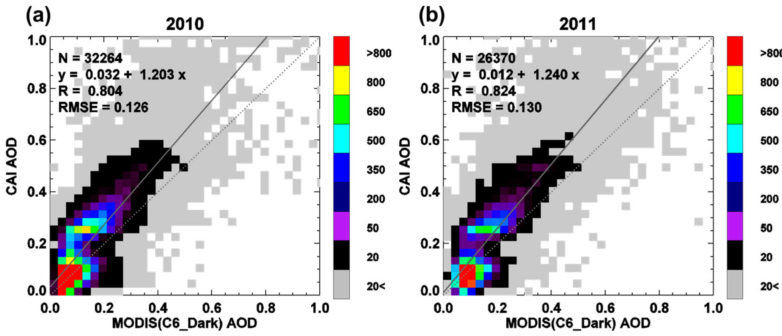
2.5. CAI Aerosol Algorithm

The YCAR-CAI algorithm uses aerosol information from the TANSO-CAI aerosol algorithm [43], which provides aerosol type and AOD at a spatial resolution of 0.1° × 0.1°. Although CAI measures globally, the YCAR-CAI algorithm is optimized over the East Asia region from 112°E to 150°E and from 24°N to 50°N because of computing resource limitations.

The YCAR-CAI algorithm selects the appropriate aerosol type from four different types of aerosol (absorbing aerosol, dust, non-absorbing aerosol, and a mixture) representing East Asia [44,45]. Aerosol properties of each type are determined by analyzing the long-term level 2 inversion products of the Aerosol Robotic NETwork (AERONET) sun-photometer observations over East Asia [46]. In the case of Global Ozone Monitoring Experiment (GOME) and Ozone Monitoring Instrument (OMI), the Aerosol Index (AI) is used to distinguish between aerosol types. However, CAI measures in only one UV band, and therefore this AI method to distinguish aerosol types is not possible to apply. Therefore, we used a reflectance difference method to determine the aerosol type. The reflectance difference between the UV band and the visible band is used to distinguish aerosol absorptivity (absorbing and non-absorbing), and the reflectance difference between the visible band and the NIR band is used to distinguish the aerosol particle size (coarse and fine). The results from the reflectance difference test of the UV and NIR bands are used to determine which of the four aerosol types are selected. After the type selection, the AODs are retrieved from the pre-calculated look-up table [45]. To improve the retrieval accuracy, surface reflectance is estimated using the clear sky composite method with a ±35-day search window for the same CAI pixels. A wider search window is used because of the insufficient number of data generated by the three-day revisit cycle of GOSAT. Furthermore, the annually estimated radiometric degradation factor of CAI is used, as suggested by Kuze et al. [47], and JAXA correction parameters using MODerate resolution Imaging Sensor (MODIS) products are also applied. Figure 1 compares retrieved AODs from MODIS and CAI for both 2010 and 2011. The results show a reasonable agreement, with correlation coefficients of 0.80–0.82 and regression slopes of about 1.2, depending on the period. More details of the algorithm and results are described in Lee et al. [43].

3. Data

FTS measurements from April 2009 to December 2012 within ±2° from Total Carbon Column Observing Network (TCCON) sites are retrieved with YCAR-CAI algorithm. The retrieved results are validated with TCCON ground-based measurements and compared with the X_CO2 retrieved by the three other algorithms (ACOS, NIES, and UoL).

3.1. TCCON

The TCCON measures the direct sun spectra in the near-infrared with ground-based FTS and has a high temporal resolution (approximately 90 s) and a high spectral resolution (approximately 0.02 cm⁻¹) [48,49]. From direct sun measurements, the TCCON retrieves not only column abundances of CO₂ (at a precision of 0.25%) but also carbon monoxide (CO), CH₄, water vapor (H₂O), and other trace gases. To guarantee consistency among different sites, the same software package, which scales the a priori profile to generate the best spectra by nonlinear least-squares fitting, is used at all TCCON stations to derive the column abundance of atmospheric gases, including CO₂ [50]. For validation, the retrieved X_CO2 is evaluated against CO₂ profiles measured by aircraft [49,51]. For the present study, we used the latest release of TCCON data, which have been updated for laser sampling error correction, spectroscopy, and air mass dependences [52]. There are four TCCON stations in northeast Asia (Anmyeondo, Rikubetsu, Saga, and Tsukuba). However, data from the recently deployed Anmyeondo and Rikubetsu stations are not used for satellite validation in this study because of the lack of long-term measurements. The characteristics of the TCCON measurement sites used in this study are summarized in

Table 2. Summary of the CO₂ datasets used in this study.

Satellite	Dates Available	Land/Ocean
YCAR-CAI	April 2009–December 2012	Land
NIES L2 v2.21	April 2009–May 2014	Both
ACOS L2 v3.4	Jun 2009–May 2013	Both
UoL-FP v6.0	April 2009–December 2014	Both
TCCON Site	Dates Available	Site Location
Tsukuba	August 2011–October 2014	36.05°N, 140.12°E
Saga	July 2011–August 2014	33.24°N, 130.29°E

.

3.2. GOSAT Retrieval

X_CO2 retrieval results from three different algorithms are compared with the results of the YCAR-CAI algorithm to identify the characteristics of the YCAR-CAI results. Data availability of each algorithm is summarized in Table 2. The ACOS and UoL-FP algorithms were developed in parallel based on the OCO algorithm and use a similar strategy, whereas the NIES operational CO₂ retrieval algorithm was developed independently. These three algorithms adopt the optimal estimation method for retrieving X_CO2 from GOSAT spectra, but the algorithms differ in many aspects, especially in the way in which aerosols are handled (

Table 3. Major differences between CO₂ retrieval algorithms.

	NIES	ACOS	UoL	YCAR-CAI
Aerosol type	Fine/Coarse mode	Water cloud, ice cloud, two aerosols	Carbon and dust, carbon and soot, cirrus	Absorbing, Non-absorbing, Mixed
Aerosol a priori	SPRINTARS	MERRA climatology	constant	CAI aerosol
Aerosol profile	logarithm	Gaussian	logarithmic	Gaussian
State vectors	CO2, aerosol, CH4, H2O, albedo, wavenumber dispersion, surface pressure, temperature bias, wind speed, adjustment factor	CO2, Aerosol, temperature offset, water vapor multiplier, surface pressure, albedo, wind speed, O2 band offset, fluorescence, residual EOF	CO2, aerosol, albedo, dispersion, zero-level offset, surface pressure, temperature offset, water vapor and CH4 multiplier, wavenumber shift	CO2, surface albedo, AOD, H2O scaling factor, surface pressure, temperature offset, wavenumber shifts and squeeze, zero-level offset
Spectroscopy	HITRAN	ABSCO	ABSCO	ABSCO
Radiative transfer model	Duan et al. 2005 [53]	LIDORT	LIDORT	VLIDORT

). These differences can result in different algorithm performances and retrieved X_CO2. For example, the aerosol transport model SPRINTARS, which is used in the NIES CO₂ retrieval algorithm, can provide more realistic a priori information than climatological studies or a constant value. This realistic a priori information is able to reduce retrieval error induced by errors in aerosol information. In the present study, post-screened GOSAT retrieval results are used without any bias correction within coincidence criteria of ±2° and ±1 h for each TCCON site.

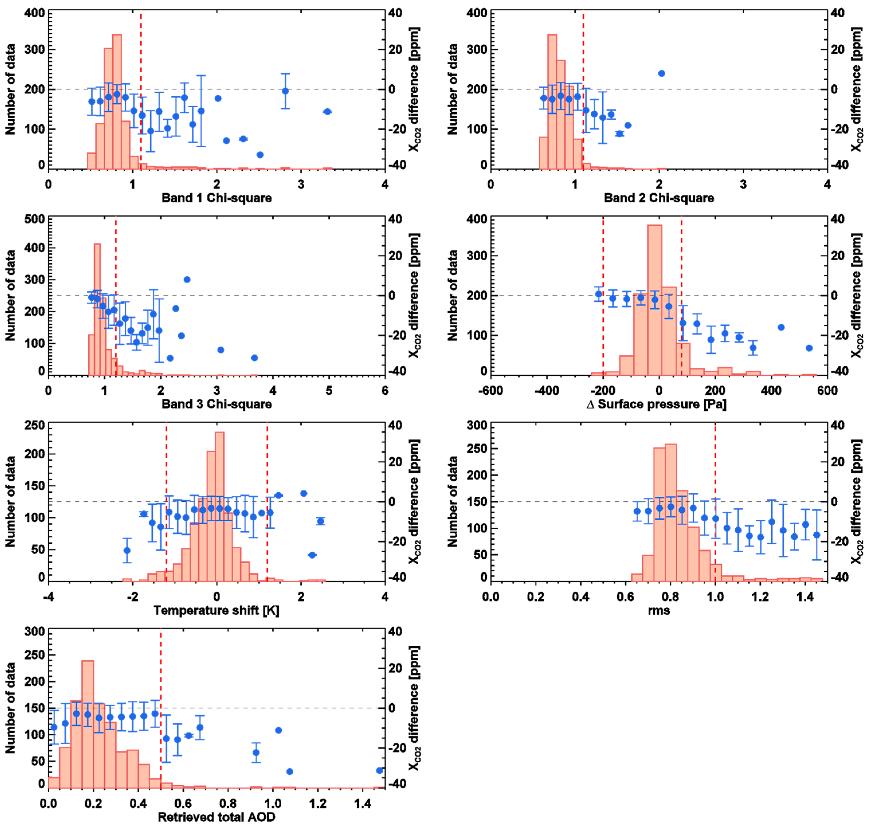
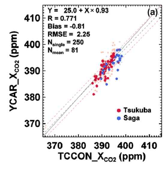
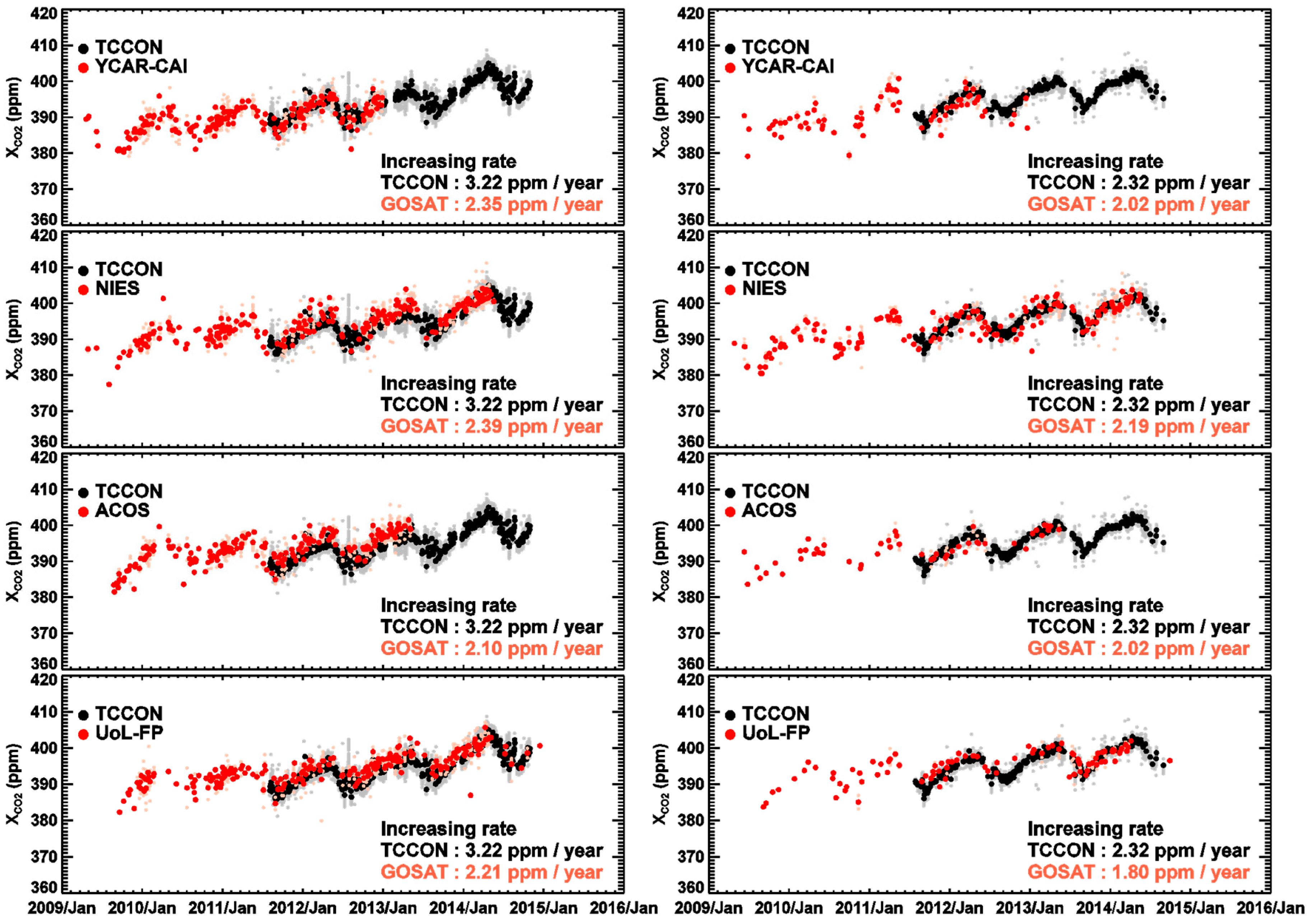
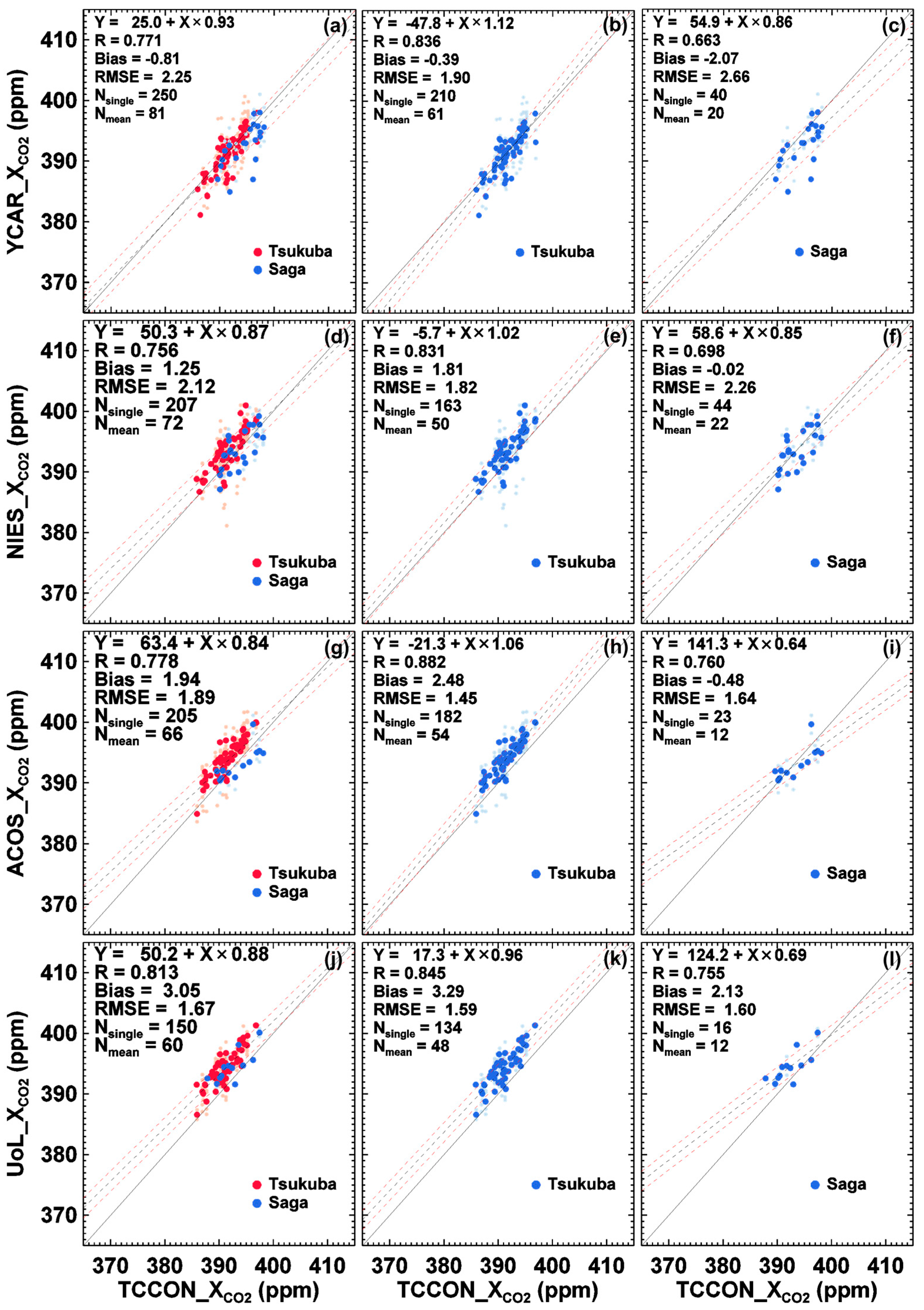
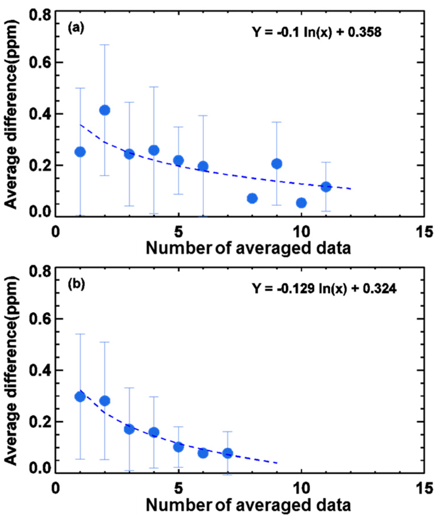
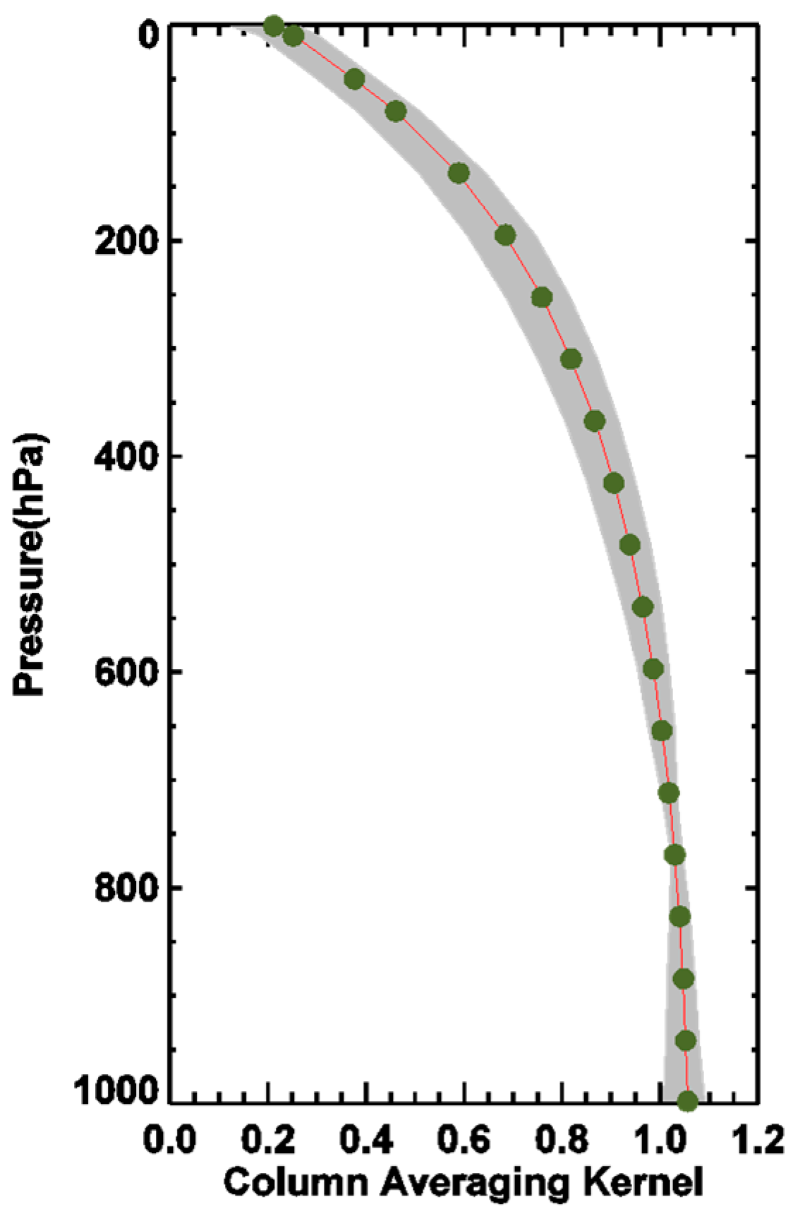
4. Results and Discussion

Table 4. Post-screening criteria.

Parameter	Criteria	Note
Chi-square of band 1	≤1.1
Chi-square of band 2	≤1.1
Chi-square of band 3	≤1.2
Surface pressure delta	−200 ≤ Pdel ≤ 80	Difference of a priori and retrieved surface pressure (Pa)
AOD	≤0.5	Retrieved AOD
Temperature shift	≤1.2 K
Root mean square	≤1

summarized the post screening criteria used for YCAR-CAI algorithm. Criteria of each component are determined based on analysis of X_CO2 difference between YCAR-CAI retrievals and TCCON measurements which is shown in Figure 2 [17,19,54,55]. The X_CO2 differences are classified into a number of groups depending on the value of each post-screening parameter. Each histogram plot shows the number of data for each rank, and the blue dots represent the average X_CO2 difference of each rank with the standard deviations being portrayed by error bars. In Figure 2, retrievals that do not meet the criteria show an increased amount of X_CO2 difference. Those results are assumed to be affected by various error sources such as cirrus cloud, measurement error, a priori error and others. Only the retrievals satisfying post screening process are used in analysis in this study.

To validate and evaluate the retrieval results of the YCAR-CAI algorithm, the results were compared with TCCON measurements and the retrievals from three different the GOSAT algorithms (NIES, ACOS, and UoL-FP). Figure 3 shows the temporal variation of X_CO2 retrievals from GOSAT algorithms and TCCON. X_CO2 data from both TCCON sites indicate evident annual CO₂ cycles with a continuous increasing trend, as shown by increasing rate in Figure 3. The annual cycle of CO₂ concentrations shows maximum values between April and June and minimum values between September and October, most likely due to the growth and decay of vegetation. The time series of X_CO2 can be assumed to be comprised of four additive subcomponents: overall mean value (${\overline{X}}_{CO2}$), a time dependent seasonal component (α), a linear trend component (β, increasing rate) and residual (R) as following equation [56].

$$X_{CO2}={\overline{X}}_{CO2}+\mathsf{\alpha }\left(t\right)+\mathsf{\beta }t+R\left(t\right)$$

(14)

X_CO2 is deseasonalized by subtracting seasonal component (α), which is estimated by harmonic analysis [57]. Then, the linear increasing rate (β) is estimated by linear least square fitting of deseasonalized X_CO2. The increasing rate of ground-based measurements is 2.32 to 3.22 ppm per year, corresponding to 16%–62% higher than the increase rate of 2 ppm measured at the Mauna Loa observatory, Hawaii (NOAA/ESRL), an established site for background CO₂ measurements [58]. Therefore, even though the general CO₂ background concentration is increasing by 2 ppm every year, the increase is higher in regions of human activity.

GOSAT retrieval results show that the CO₂ concentration is increasing between 2.10 and 2.39 ppm per year at the Tsukuba monitoring site. At the Saga monitoring site, the GOSAT retrieval results show that the CO₂ concentration is increasing by 1.80–2.19 ppm per year. In both site, NIES and YCAR-CAI shows highest and second highest increasing rate. In addition, all the GOSAT algorithm and TCCON shows higher increasing rate at Tsukuba than Saga. However, the increases indicated by the GOSAT algorithms at Saga are less certain than those at Tsukuba because of insufficient coincident data. The Saga site is located in a rural area close to the ocean with a complicated coastline, which reduces the number of GOSAT measurements available for retrieval, and thus produces fewer X_CO2 data. For this reason, the Saga site shows a small standard deviation for TCCON data and a small number of available GOSAT retrievals. Conversely, the Tsukuba site is adjacent to the Tokyo metropolitan area and is an inland location reasonably close to the Pacific Ocean. Therefore, the Tsukuba site is influenced by two different areas with dissimilar air quality characteristics. This geographical position induces higher deviations of CO₂ concentrations and a greater number of available GOSAT measurements when compared with the Saga site. Higher increasing rate at Tsukuba is probably also due to the influence of the metropolitan area.

Figure 4 shows a comparison of GOSAT X_CO2 with TCCON X_CO2 for both sites (Tsukuba and Saga). To compare the retrieval results for the same period under the same conditions, GOSAT data without any bias correction were compared for the period April 2009 to December 2012, when GOSAT X_CO2 retrievals are available for all algorithms. As shown in Figure 4a, the YCAR-CAI algorithm regression line lies closer to the linear identity function compared with the lines of the other retrieval algorithms. The YCAR-CAI algorithm has the largest available retrieval dataset (250 individual soundings and 81 daily averaged data values) compared with the other retrieval algorithms. The other retrieval algorithms screen out a higher percentage of retrieved data because of the effect of aerosols and clouds, whereas the YCAR-CAI algorithm maintains a large dataset. Although the YCAR-CAI algorithm has the largest dataset, the regression analysis results, such as the coefficient of determination, bias, and root-mean-square error (RMSE) values, are still comparable with those of other algorithms. The UoL-FP algorithm shows the lowest RMSE but has the smallest dataset, meaning that large portions of the data are screened out by tight criteria. All the algorithms have a coefficient of determination of 0.756–0.813, whereas that of YCAR-CAI is 0.771. The RMSE of YCAR-CAI is 2.28, whereas those of the other algorithms range between 1.67 and 2.12. These results show the reliability and accuracy of the YCAR-CAI algorithm.

Figure 4 also shows a comparison of GOSAT X_CO2 and TCCON X_CO2 for each of the two studied TCCON sites. For Tsukuba, the results of the all algorithms shows regression slopes of 0.96–1.12 all being nearly parallel to the linear identity function. The YCAR-CAI results show slight underestimates compared with TCCON, with the small absolute bias of −0.39 ppm and a regression slope of 1.12. The RMSEs for the algorithms range between 1.45 and 1.82 ppm, with the ACOS algorithm being the lowest. For the Saga site, the ACOS and UoL-FP algorithms have an insufficient number of data coincident with TCCON to conduct validation and are thus discounted. The YCAR-CAI and NIES algorithms show regression slopes of 0.86 and 0.85, respectively. NIES algorithm shows slightly higher number of available data but similar with that of YCAR-CAI algorithm.

The overall validation results of YCAR-CAI algorithm are improved or comparable with other algorithms. These improvements are probably due to the various components and characteristic of YCAR-CAI algorithm. Among those characteristics, aerosol information is most influential factor for X_CO2 retrieval, so YCAR-CAI retrieval is improved largely due to a priori CAI aerosol information. Errors in a priori information could be propagated to other state vector elements in the retrieval process and some of those retrievals could be screened out while post screening process due to the propagated error. Simultaneous aerosol information from CAI algorithm reduced aerosol induced error and CT-A data, which is optimized to East Asia, minimized CO₂ a priori induced error. Minimization of a priori error reduces the error propagations and helps the iterations converge closer to the true value. For those reason, YCAR-CAI algorithm shows higher number of available data and correlation with TCCON measurements.

There are both spatial and temporal differences between TCCON and GOSAT measurements, meaning that the GOSAT algorithms cannot have the same results as TCCON. Using model simulations, Kulawik et al. [59] analyzed the sampling errors induced by the spatio-temporal mismatch between satellites and TCCON. In a similar manner, we analyzed the spatio-temporal sampling error over East Asia TCCON sites with CT-A data (see Figure 5). For error analysis, we compared CT-A at GOSAT time and location with CT-A at TCCON time and location. The spatio-temporal sampling errors are daily averaged, and the averaged values are grouped by the number of data used in averaging. The mean values of each group are displayed in Figure 5, with standard deviations shown as error bars. Dashed lines represent the logarithmic least square fit curve, which shows that a decrease in error depends on the number of averaged data points. According to the fit curve, each individual measurement from GOSAT has an average difference of 0.32 to 0.36 ppm compared with TCCON measurements, with the difference being caused by the spatio-temporal sampling difference. This difference can be canceled out by averaging the data that satisfy coincidence criteria. In Figure 5b, the sampling error for the Saga site decreases with the number of averaged data, as does the standard deviation. The Saga site shows a smaller sampling error and fitting residual compared with the Tsukuba site. The larger sampling error and fitting residual for the Tsukuba site is because there is a larger spatio-temporal variability measured at Tsukuba. However, for the Saga site, fewer individual sounding data are daily averaged for validation because of the shortage of coincident data. Figure 4 shows that for Saga, the YCAR-CAI algorithm has 40 individual soundings that are then computed into 20 daily averaged CO₂ concentrations, resulting in about two individual soundings coinciding with TCCON measurements each day. For Tsukuba, 210 individual soundings are averaged into 61 daily averaged CO₂ concentrations, thus yielding about 75% more coincident individual soundings each day compared with Saga. Therefore, Saga site has a similar sampling error compared with the Tsukuba site.

Figure 6 presents the column averaging kernel corresponding to the YCAR-CAI retrieval results shown in Figure 3 and Figure 4. All the column averaging kernels are included in the shaded area, and the solid line represents the mean value of the column averaging kernels. Generally speaking, a column averaging kernel value of about 1 means that the a priori values scarcely affect the retrieved values. In Figure 6, the column averaging kernel is about 1.05 at the surface and decreases slightly through the pressure levels, until 400 hPa, from where it decreases markedly with lower pressure. This means that the retrieved values are highly sensitive to CO₂ concentrations from the near surface to the 400 hPa layer, but are highly constrained by a priori information at high altitudes where the atmospheric pressure is lower than 400 hPa. However, most of the CO₂ sources and sinks are located near the surface, where the averaging kernel shows higher values, and the CO₂ concentrations at high altitude are relatively consistent and well known. Therefore, although the value of the column averaging kernel is low for this attitude range and the YCAR-CAI algorithm has a low sensitivity to high-altitude CO₂ concentration, the accuracy of the retrieval results is not severely affected.

The variance of X_CO2 due to measurement noise, smoothing and interference is calculated using Equations (10)–(13) and summarized in

Table 5. Averaged values of variance components for two TCCON sites.

Variance	Tsukuba (ppm2)	Saga (ppm2)
Total	1.93	2.19
Measurement	1.37	1.61
Smoothing	0.41	0.37
Interference	0.15	0.21

. The total variance of retrieval results of the YCAR-CAI algorithm is 1.93 and 2.19 ppm² at Tsukuba and Saga, respectively, which correspond to 1.39 and 1.48 ppm of uncertainty in YCAR-CAI retrieval. Total variance at Saga is slightly higher than that of Tsukuba, which means retrievals over Saga have higher retrieval uncertainty. Large portion of total variance is induced by measurement and relatively small amount of variance is induced by smoothing and interference.

5. Summary and Conclusions

We developed the YCAR-CAI X_CO2 retrieval algorithm for GOSAT TANSO-FTS measurements using simultaneous TANSO-CAI aerosol information to reduce the retrieval error and increase the number of retrieved data points over East Asia, where aerosol amounts are consistently high. This paper has provided details of YCAR-CAI algorithm along with validation results. Previous algorithms have used either transport model results or climatological values for aerosols, which have geographical and temporal differences with the GOSAT FTS measurements. The aerosol type and optical depth information from the TANSO-CAI AOD algorithm were simultaneously retrieved for the same geometry and optical path as TANSO-FTS. The aerosol information was used as a priori information to reduce the retrieval error of X_CO2. CT-A data optimized to the East Asia region were used as a priori information for CO₂ to improve the reliability of a priori information.

YCAR-CAI retrieval results were validated against TCCON ground-based measurements and compared with X_CO2 results from the NIES, ACOS, and UoL-FP algorithms. The GOSAT data (without bias correction) and TCCON data were compared for the period April 2009 to December 2012. Regarding the temporal variation of X_CO2, the GOSAT retrieval results show an annual cycle, with a maximum between April and June and a minimum between September and October. There is a continuously increasing trend of between 2.02 and 2.39 ppm of CO₂ per year. In both sites, TCCON shows higher increasing rate than GOSAT. Moreover, all the datasets shows higher increasing rate in Tsukuba than Saga.

The data sample size of the YCAR-CAI algorithm exceeds that of other retrieval algorithms by 21% to 67%, and the regression results are comparable with those of other algorithms. Of the four algorithms compared, the YCAR-CAI algorithm shows a regression line closest to the linear identity function, with a regression slope of 0.93 and an intercept of 25. Other regression statistics, such as the coefficient of determination, absolute bias, and RMSE value, are also comparable with the other algorithms.

We also examined variance components of retrieval results, which consist of variance of X_CO2 due to measurement, smoothing and interference error. The YCAR-CAI algorithm shows total variance of 1.93 and 2.19 ppm² of X_CO2 at Tsukuba and Saga, respectively, which means YCAR-CAI has uncertainty of 1.39 and 1.48 ppm over the two TCCON sites. Most of the uncertainty is due to measurement errors, which are caused by noise in the measured spectrum. The next generation of greenhouse-gas-observing satellites should improve measurement accuracy to allow reducing the retrieval error. We also examined the error caused by spatio-temporal differences between satellite and ground-based measurements using CT-A data. Here, the error caused by spatio-temporal sampling is between 0.32 and 0.36 ppm on average. This error can be improved only by having more multiple coincidence data for averaging. Therefore, a larger number of available X_CO2 data, as provided using the YCAR-CAI algorithm, has the advantage of reducing the spatio-temporal sampling error and improving the analysis of CO₂ trends.

The present study suggests a different strategy in aerosol information for X_CO2 retrieval. YCAR-CAI algorithm uses simultaneous aerosol information retrieved from CAI as a priori data and the retrievals show reliable validation results and also show consistent CO₂ variation trends with TCCON dataset over East Asia. Given the importance of monitoring CO₂ concentrations, various greenhouse-gas-monitoring satellites are planned, such as TANSAT, GOSAT-2, and OCO-3. This study can provide alternative approach to retrieve X_CO2 using simultaneous aerosol information for future satellite missions. In future studies, we intend to refine detailed processes such as cloud handling and other aspects of the aerosol algorithm. Furthermore, we intend conducting retrievals over a wider area and for a longer period by improving the computational cost.

References

1. Intergovernmental Panel on Climate Change (IPCC). Climate Change 2014: Synthesis Report. Contribution of Working Groups I, II and III to the Fifth Assessment Report of the Intergovernmental Panel on Climate Change; IPCC: Geneva, Switzerland, 2014. [Google Scholar]
2. Masarie, K.A.; Tans, P.P. Extension and integration of atmospheric carbon-dioxide data into a globally consistent measurement record. J. Geophys. Res. Atmos. 1995, 100, 11593–11610. [Google Scholar] [CrossRef]
3. Solomon, S.; Intergovernmental Panel on Climate Change; Intergovernmental Panel on Climate Change, Working Group I. Climate Change 2007: The Physical Science Basis: Contribution of Working Group I to the Fourth Assessment Report of the Intergovernmental Panel on Climate Chang; Cambridge University Press: Cambridge, UK; New York, NY, USA, 2007; p. 996. [Google Scholar]
4. Jones, N. Troubling milestone for CO2. Nat. Geosci. 2013, 6, 589. [Google Scholar] [CrossRef]
5. Wigley, T.M.L. The pre-industrial carbon-dioxide level. Clim. Chang. 1983, 5, 315–320. [Google Scholar] [CrossRef]
6. Schmidt, H.; Alterskjaer, K.; Karam, D.B.; Boucher, O.; Jones, A.; Kristjansson, J.E.; Niemeier, U.; Schulz, M.; Aaheim, A.; Benduhn, F.; et al. Solar irradiance reduction to counteract radiative forcing from a quadrupling of CO2: Climate responses simulated by four earth system models. Earth Syst. Dyn. 2012, 3, 63–78. [Google Scholar] [CrossRef] [Green Version]
7. Keeling, C.D. The concentration and isotopic abundances of carbon dioxide in the atmosphere. Tellus 1960, 12, 200–203. [Google Scholar] [CrossRef]
8. World Meteorological Organization (WMO). Strategy for the Implementation of the Global Atmosphere Watch Programme (2001–2007), a Contribution to the Implementation of the WMO Long-Term Plan; WMO: Geneva, Switzeland, 2001. [Google Scholar]
9. World Meteorological Organization (WMO). World Data Center for Greenhouse Gases (WDCGG) Data Summary; WDCGG: Tokyo, Japan, 2012. [Google Scholar]
10. Conway, T.; Lang, P.; Masarie, K. Atmospheric Carbon Dioxide Dry Air Mole Fractions from the Noaa Esrl Carbon Cycle Cooperative Global Air Sampling Network, 1968–2006, Version: 2007–09–19. Available online: https://www.ftp.cmdl.noaa.gov/ccg/co2/flask/event (accessed on 30 November 2016).
11. Conway, T.; Tans, P.P.; Waterman, L.; Thoning, K.; Kitzis, D.; Masarie, K.; Zhang, N. Evidence for interannual variability of the carbon cycle from the noaa/cmdl global air sampling network. J. Geophys. Res. 1994, 99, 22831–22855. [Google Scholar] [CrossRef]
12. Hungershoefer, K.; Breon, F.M.; Peylin, P.; Chevallier, F.; Rayner, P.; Klonecki, A.; Houweling, S.; Marshall, J. Evaluation of various observing systems for the global monitoring of CO2 surface fluxes. Atmos. Chem. Phys. 2010, 10, 10503–10520. [Google Scholar] [CrossRef]
13. Gurney, K.R.; Law, R.M.; Denning, A.S.; Rayner, P.J.; Baker, D.; Bousquet, P.; Bruhwiler, L.; Chen, Y.H.; Ciais, P.; Fan, S.; et al. Towards robust regional estimates of CO2 sources and sinks using atmospheric transport models. Nature 2002, 415, 626–630. [Google Scholar] [CrossRef] [PubMed]
14. Yokota, T.; Yoshida, Y.; Eguchi, N.; Ota, Y.; Tanaka, T.; Watanabe, H.; Maksyutov, S. Global concentrations of CO2 and ch4 retrieved from GOSAT: First preliminary results. Sola 2009, 5, 160–163. [Google Scholar] [CrossRef]
15. Crisp, D. Measuring atmospheric carbon dioxide from space with the orbiting carbon observatory-2 (oco-2). In SPIE Optical Engineering+ Applications; International Society for Optics and Photonics: Bellingham, WA, USA, 2015; pp. 960702–960707. [Google Scholar]
16. Kuze, A.; Suto, H.; Nakajima, M.; Hamazaki, T. Thermal and near infrared sensor for carbon observation fourier-transform spectrometer on the greenhouse gases observing satellite for greenhouse gases monitoring. Appl. Opt. 2009, 48, 6716–6733. [Google Scholar] [CrossRef] [PubMed]
17. Yoshida, Y.; Ota, Y.; Eguchi, N.; Kikuchi, N.; Nobuta, K.; Tran, H.; Morino, I.; Yokota, T. Retrieval algorithm for CO2 and CH4 column abundances from short-wavelength infrared spectral observations by the greenhouse gases observing satellite. Atmos. Meas. Tech. 2011, 4, 717–734. [Google Scholar] [CrossRef]
18. Connor, B.J.; Boesch, H.; Toon, G.; Sen, B.; Miller, C.; Crisp, D. Orbiting carbon observatory: Inverse method and prospective error analysis. J. Geophys. Res. Atmos. 2008, 113. [Google Scholar] [CrossRef]
19. Crisp, D.; Fisher, B.M.; O’Dell, C.; Frankenberg, C.; Basilio, R.; Bosch, H.; Brown, L.R.; Castano, R.; Connor, B.; Deutscher, N.M.; et al. The acos CO2 retrieval algorithm—Part ii: Global x-CO2 data characterization. Atmos. Meas. Tech. 2012, 5, 687–707. [Google Scholar] [CrossRef]
20. O’Dell, C.W.; Connor, B.; Bosch, H.; O’Brien, D.; Frankenberg, C.; Castano, R.; Christi, M.; Crisp, D.; Eldering, A.; Fisher, B.; et al. The acos CO2 retrieval algorithm—Part 1: Description and validation against synthetic observations. Atmos. Meas. Tech. 2012, 5, 99–121. [Google Scholar] [CrossRef]
21. Boesch, H.; Baker, D.; Connor, B.; Crisp, D.; Miller, C. Global characterization of CO2 column retrievals from shortwave-infrared satellite observations of the orbiting carbon observatory-2 mission. Remote Sens. 2011, 3, 270–304. [Google Scholar] [CrossRef]
22. Butz, A.; Hasekamp, O.P.; Frankenberg, C.; Aben, I. Retrievals of atmospheric CO2 from simulated space-borne measurements of backscattered near-infrared sunlight: Accounting for aerosol effects. Appl. Opt. 2009, 48, 3322–3336. [Google Scholar] [CrossRef] [PubMed]
23. Saitoh, N.; Imasu, R.; Ota, Y.; Niwa, Y. CO2 retrieval algorithm for the thermal infrared spectra of the greenhouse gases observing satellite: Potential of retrieving CO2 vertical profile from high-resolution fts sensor. J. Geophys. Res. Atmos. 2009, 114. [Google Scholar] [CrossRef]
24. Oshchepkov, S.; Bril, A.; Yokota, T.; Morino, I.; Yoshida, Y.; Matsunaga, T.; Belikov, D.; Wunch, D.; Wennberg, P.; Toon, G.; et al. Effects of atmospheric light scattering on spectroscopic observations of greenhouse gases from space: Validation of ppdf-based CO2 retrievals from gosat. J. Geophys. Res. Atmos. 2012, 117. [Google Scholar] [CrossRef]
25. Frankenberg, C.; Platt, U.; Wagner, T. Iterative maximum a posteriori (imap)-doas for retrieval of strongly absorbing trace gases: Model studies for CH4 and CO2 retrieval from near infrared spectra of sciamachy onboard envisat. Atmos. Chem. Phys. 2005, 5, 9–22. [Google Scholar] [CrossRef]
26. O’Brien, D.M.; Rayner, P.J. Global observations of the carbon budge—2. CO2 column from differential absorption of reflected sunlight in the 1.61 mu m band of CO2. J. Geophys. Res. Atmos. 2002, 107. [Google Scholar] [CrossRef]
27. Takemura, T.; Okamoto, H.; Maruyama, Y.; Numaguti, A.; Higurashi, A.; Nakajima, T. Global three-dimensional simulation of aerosol optical thickness distribution of various origins. J. Geophys. Res. Atmos. 2000, 105, 17853–17873. [Google Scholar] [CrossRef]
28. ESA Greenhouse Gas-Climate Change Initiative (GHG-CCI). Algorithm Theoretical Basis Document Version 3 (atbdv3)—The University of Leicester Fullphysics Retrieval Algorithm for the Retrieval of xCO2 and xCH4; ESA Greenhouse Gas-Climate Change Initiative (GHG-CCI): Paris, France, 2014; pp. 1–28. [Google Scholar]
29. Boesch, H.; Vogel, L.; Hewson, W.; Parker, R.; Somkuti, P.; Sembhi, H.; Webb, A. An Improved Aerosol Scheme for the GHG Retrieval from GOSAT. In Proceedings of the 12th International Workshop on Greenhouse Gas Measurements from Space, Kyoto, Japan, 7–9 June 2016.
30. Kuze, A.; Urabe, T.; Suto, H.; Kaneko, Y.; Hamazaki, T. The instrumentation and the BBM test results of thermal and near-infrared sensor for carbon observation (TANSO) on GOSAT. In SPIE Optics+ Photonics; International Society for Optics and Photonics: Bellingham, WA, USA, 2006; pp. 62970K–62978K. [Google Scholar]
31. Kuang, Z.M.; Margolis, J.; Toon, G.; Crisp, D.; Yung, Y. Spaceborne measurements of atmospheric CO2 by high-resolution nir spectrometry of reflected sunlight: An introductory study. Geophys. Res. Lett. 2002, 29. [Google Scholar] [CrossRef]
32. Boesche, E.; Stammes, P.; Bennartz, R. Aerosol influence on polarization and intensity in near-infrared o-2 and CO2 absorption bands observed from space. J. Quant. Spectrosc. Radiat. Transf. 2009, 110, 223–239. [Google Scholar] [CrossRef]
33. Houweling, S.; Hartmann, W.; Aben, I.; Schrijver, H.; Skidmore, J.; Roelofs, G.J.; Breon, F.M. Evidence of systematic errors in sciamachy-observed CO2 due to aerosols. Atmos. Chem. Phys. 2005, 5, 3003–3013. [Google Scholar] [CrossRef] [Green Version]
34. Mao, J.P.; Kawa, S.R. Sensitivity studies for space-based measurement of atmospheric total column carbon dioxide by reflected sunlight. Appl. Opt. 2004, 43, 914–927. [Google Scholar] [CrossRef] [PubMed]
35. Rodgers, C.D. Inverse Methods for Atmospheric Sounding: Theory and Practice; World Scientific: Singapore, 2000; Volume 2. [Google Scholar]
36. Jung, Y.; Kim, J.; Kim, W.; Boesch, H.; Lee, H.; Cho, C.; Goo, T.Y. Impact of aerosol property on the accuracy of a CO2 retrieval algorithm from satellite remote sensing. Remote Sens. 2016, 8, 20. [Google Scholar] [CrossRef]
37. Levenberg, K. A method for the solution of certain non–linear problems in least squares. 1944, 2, 164–168. [Google Scholar]
38. Marquardt, D.W. An algorithm for least-squares estimation of nonlinear parameters. J. Soc. Ind. Appl. Math. 1963, 11, 431–441. [Google Scholar] [CrossRef]
39. Spurr, R.J.D. Vlidort: A linearized pseudo-spherical vector discrete ordinate radiative transfer code for forward model and retrieval studies in multilayer multiple scattering media. J. Quant. Spectrosc. Radiat. Transf. 2006, 102, 316–342. [Google Scholar] [CrossRef]
40. Bodhaine, B.A.; Wood, N.B.; Dutton, E.G.; Slusser, J.R. On Rayleigh optical depth calculations. J. Atmos. Ocean. Tech. 1999, 16, 1854–1861. [Google Scholar] [CrossRef]
41. Tran, H.; Hartmann, J.M. An improved o-2 a band absorption model and its consequences for retrievals of photon paths and surface pressures. J. Geophys. Res. Atmos. 2008, 113. [Google Scholar] [CrossRef]
42. Toon, G.C.; Blavier, J.F.; Sen, B.; Salawitch, R.J.; Osterman, G.B.; Notholt, J.; Rex, M.; McElroy, C.T.; Russell, J.M. Ground-based observations of arctic o-3 loss during spring and summer 1997. J. Geophys. Res. Atmos. 1999, 104, 26497–26510. [Google Scholar] [CrossRef]
43. Lee, S.; Kim, J.; Kim, M.; Choi, M.; Go, S.; Lim, H.; Goo, T.; Tatsuya, Y. Development of aerosol retrieval algorithm over East Asia from TANSO-CAI measurements onboard GOSAT. Unpublished work. 2017. [Google Scholar]
44. Higurashi, A.; Nakajima, T. Detection of aerosol types over the East China Sea near Japan from four-channel satellite data. Geophys. Res. Lett. 2002, 29. [Google Scholar] [CrossRef]
45. Kim, J.; Lee, J.; Lee, H.C.; Higurashi, A.; Takemura, T.; Song, C.H. Consistency of the aerosol type classification from satellite remote sensing during the atmospheric brown cloud-east asia regional experiment campaign. J. Geophys. Res. Atmos. 2007, 112. [Google Scholar] [CrossRef]
46. Lee, J.; Kim, J.; Song, C.H.; Kim, S.B.; Chun, Y.; Sohn, B.J.; Holben, B.N. Characteristics of aerosol types from aeronet sunphotometer measurements. Atmos. Environ. 2010, 44, 3110–3117. [Google Scholar] [CrossRef]
47. Kuze, A.; Taylor, T.E.; Kataoka, F.; Bruegge, C.J.; Crisp, D.; Harada, M.; Helmlinger, M.; Inoue, M.; Kawakami, S.; Kikuchi, N.; et al. Long-term vicarious calibration of GOSAT short-wave sensors: Techniques for error reduction and new estimates of radiometric degradation factors. IEEE Trans. Geosci. Remote Sens. 2014, 52, 3991–4004. [Google Scholar] [CrossRef]
48. Wunch, D.; Toon, G.C.; Blavier, J.F.L.; Washenfelder, R.A.; Notholt, J.; Connor, B.J.; Griffith, D.W.T.; Sherlock, V.; Wennberg, P.O. The total carbon column observing network. Philos. Trans. R. Soc. A Math. Phys. Eng. Sci. 2011, 369, 2087–2112. [Google Scholar] [CrossRef] [PubMed]
49. Wunch, D.; Toon, G.C.; Wennberg, P.O.; Wofsy, S.C.; Stephens, B.B.; Fischer, M.L.; Uchino, O.; Abshire, J.B.; Bernath, P.; Biraud, S.C.; et al. Calibration of the total carbon column observing network using aircraft profile data. Atmos. Meas. Tech. 2010, 3, 1351–1362. [Google Scholar] [CrossRef] [Green Version]
50. Geibel, M.C.; Messerschmidt, J.; Gerbig, C.; Blumenstock, T.; Chen, H.; Hase, F.; Kolle, O.; Lavric, J.V.; Notholt, J.; Palm, M.; et al. Calibration of column-averaged ch4 over european tccon fts sites with airborne in-situ measurements. Atmos. Chem. Phys. 2012, 12, 8763–8775. [Google Scholar] [CrossRef]
51. Messerschmidt, J.; Geibel, M.C.; Blumenstock, T.; Chen, H.; Deutscher, N.M.; Engel, A.; Feist, D.G.; Gerbig, C.; Gisi, M.; Hase, F.; et al. Calibration of TCCON column-averaged CO2: The first aircraft campaign over european tccon sites. Atmos. Chem. Phys. 2011, 11, 10765–10777. [Google Scholar] [CrossRef]
52. Wunch, D.; Toon, G.C.; Sherlock, V.; Deutscher, N.M.; Liu, X.; Feist, D.G.; Wennberg, P.O. The total carbon column observing network’s GGG2014 data version. Carbon Dioxide Inf. Anal. Cent. 2015, 43. [Google Scholar] [CrossRef]
53. Duan, M.Z.; Min, Q.L.; Li, J.N. A fast radiative transfer model for simulating high-resolution absorption bands. J. Geophys. Res. Atmos. 2005, 110. [Google Scholar] [CrossRef]
54. Cogan, A.J.; Boesch, H.; Parker, R.J.; Feng, L.; Palmer, P.I.; Blavier, J.F.L.; Deutscher, N.M.; Macatangay, R.; Notholt, J.; Roehl, C.; et al. Atmospheric carbon dioxide retrieved from the greenhouse gases observing satellite (GOSAT): Comparison with ground-based tccon observations and geos-chem model calculations. J. Geophys. Res. Atmos. 2012, 117. [Google Scholar] [CrossRef]
55. Boesch, H.; Toon, G.C.; Sen, B.; Washenfelder, R.A.; Wennberg, P.O.; Buchwitz, M.; de Beek, R.; Burrows, J.P.; Crisp, D.; Christi, M.; et al. Space-based near-infrared CO2 measurements: Testing the orbiting carbon observatory retrieval algorithm and validation concept using sciamachy observations over park falls, wisconsin. J. Geophys. Res. Atmos. 2006, 111. [Google Scholar] [CrossRef]
56. Lamsal, L.N.; Duncan, B.N.; Yoshida, Y.; Krotkov, N.A.; Pickering, K.E.; Streets, D.G.; Lu, Z.F.U.S. NO2 trends (2005–2013): Epa Air Quality System (AQS) data versus improved observations from the ozone monitoring instrument (OMI). Atmos. Environ. 2015, 110, 130–143. [Google Scholar] [CrossRef]
57. Wilks, D.S. Statistical Methods in the Atmospheric Sciences; Academic Press: Amsterdam, The Netherlands, 2011; Volume 100. [Google Scholar]
58. Tans, P.; Keeling, R. ESRL Global Monitoring Divisioneglobal Greenhouse Gas Reference Network. Available online: http://www.esrl.noaa.gov/gmd/ccgg/obspack/release_notes.html (accessed on 30 November 2016).
59. Kulawik, S.; Wunch, D.; O’Dell, C.; Frankenberg, C.; Reuter, M.; Oda, T.; Chevallier, F.; Sherlock, V.; Buchwitz, M.; Osterman, G. Consistent evaluation of GOSAT, sciamachy, carbontracker, and MACC through comparisons to TCCON. Atmos. Meas. Tech. 2015, 8, 6217–6277. [Google Scholar] [CrossRef]
Figure 1. Comparisons of retrieved AOD from MODIS and TANSO-CAI over ocean in: (a) 2010; and (b) 2011. Colors represent the frequency of compared results.
Remotesensing 08 00994 g001
Figure 2. The relation between XCO2 difference (XCO2, GOSAT—XCO2, TCCON) and filter variables. Blue dots are mean XCO2 difference of each bin with error bar of standard deviation. Red line represents post screening criteria.
Remotesensing 08 00994 g002
Figure 3. Time series of retrieved XCO2 from four GOSAT algorithms (YCAR-CAI, NIES, ACOS, and UoL, from top to bottom, respectively) and from two TCCON sites (Tsukuba (left) and Saga (right)). All TCCON retrieved data are shown in small gray dots and daily average TCCON XCO2 values within 1 h of GOSAT passing times (approximately 12:50 UTC at East Asia TCCON sites) are shown in large black dots.
Remotesensing 08 00994 g003
Figure 4. Comparison of retrieved XCO2 from four GOSAT algorithms ((ac) YCAR-CAI; (df) NIES; (gi) ACOS; and (jl) UoL) with TCCON XCO2 for two TCCON sites: Tsukuba (middle), Saga (right), and both (left). All individual sounding GOSAT data are shown as small faded dots, and daily average values are shown as large distinct colored dots. Black dotted line is the best-fit line calculated from robust fitting and red dotted lines are RMSE range of best-fit line. The solid line is linear identity function.
Remotesensing 08 00994 g004
Figure 5. Error induced by spatio-temporal sampling error over: (a) Tsukuba; and (b) Saga TCCON sites, with the standard deviation given by error bars. The dashed line represents the logarithmic least square fit curve.
Remotesensing 08 00994 g005
Figure 6. An example of a column averaging kernel for YCAR-CAI CO2 retrieval. The shaded area indicates the variation range of the column averaging kernel over the Tsukuba and Saga TCCON sites. The solid line with dots shows the mean column averaging kernel.
Remotesensing 08 00994 g006