Article

Stage Monitoring in Turbid Reservoirs with an Inclined Terrestrial Near-Infrared Lidar

by
Serge Tamari
1,*,
Vicente Guerrero-Meza
2,
Younès Rifad
3,
Luis Bravo-Inclán
1 and
José Javier Sánchez-Chávez
1
1
Instituto Mexicano de Tecnología del Agua (IMTA), Paseo Cuauhnáhuac No. 8532, Col. Progreso, Jiutepec Mor. 62550, Mexico
2
DISIME S.A. de C.V., Playa Villa del Mar No. 180, Col. Militar Marte, Ciudad de México D.F. 08830, Mexico
3
Ecole des Mines de Douai (EMD), 941 rue Charles Bourseul, Douai 59508, France
*
Author to whom correspondence should be addressed.
Remote Sens. 2016, 8(12), 999; https://doi.org/10.3390/rs8120999
Submission received: 26 September 2016 / Revised: 11 November 2016 / Accepted: 23 November 2016 / Published: 6 December 2016

Abstract

:
To monitor the stage in turbid reservoirs with a sloping bank, it has been proposed to install a near-infrared Lidar on the bank and to orient it so that it points at the water surface with a large incidence angle (between ≈ 30° and 70°). The technique assumes that the Lidar can detect suspended particles that are slightly below the water surface. Some laboratory results and the first long-term assessment (>2 years) of the technique are presented. It found that: (1) although the test Lidar provides erratic distance data, they can be easily filtered according to the intensity of the received signal; (2) the Lidar provides reliable data only when the water is very turbid (Secchi depth smaller than ≈ 1.0 m); and (3) the reliable data can be used to estimate daily stage values (after a simple field calibration) with an uncertainty better than ±0.08 m (p = 0.95). Although the present form of the technique is not very accurate, it uses an inexpensive instrument (≈1500 USD) which can be easily installed in a safe place (such as is the roof of a building). It is argued that the technique could be also used to monitor the stage and the sub-surface velocity in others turbid water bodies, such as some coastal areas (a recent field of application) and flooding rivers.

Graphical Abstract

1. Introduction

As discussed by Tamari et al. [1], it is sometimes difficult to use the current terrestrial techniques or airborne instruments for monitoring the stage of reservoirs with a sloping bank (such as many lakes and earth-dam embankments). Therefore, it would be useful to develop techniques that can monitor the stage using non-contact terrestrial instruments mounted at the edge and that look at the water surface with a large incidence angle (typically larger than ≈ 60°). In the particular case of turbid reservoirs, Tamari et al. [1] have proposed a new technique using a (time-of-flight) inclined near-infrared Lidar. This technique is based on two simple assumptions about the so-called “volume scattering” (e.g., [2]): (1) the main feature that can be detected by a Lidar looking with a large incidence angle (between ≈ 30° and 70°) at a turbid water body (with no floating objects) are suspended particles (due to the Tyndall effect) and (2) those detected particles—if any—should be slightly below the water surface (due to the strong absorption of the near-infrared light by water, if compared to other Lidar wavelengths).
The basic assumptions of the proposed technique are not new: as a matter of fact, Churnside and Palmer [2] have suggested 20 years ago that they could be used for monitoring some coastal areas. A few authors have also presented qualitative observations suggesting that they could be applied to certain rivers [3,4]. However, for some reasons discussed at the end of this study, these assumptions have been almost exclusively applied under laboratory conditions, that is, with artificially-prepared turbid water [1,2,4,5,6,7]. As far as we know, the only field testing of the proposed technique is the one reported by Tamari et al. [1]. It must be recognized that some commercial systems using an inclined Lidar—known as the Terrestrial Laser Scanning (TLS) systems—are getting popular for monitoring the stage of some coastal areas and rivers; however, and as discussed later, these systems are not explicitly based on the two assumptions considered during this study.
The field testing of the proposed technique made by Tamari et al. [1] was only a proof of concept; as a matter of fact, it was performed: (1) with one simple Lidar model of a given brand; (2) configured in one mode only (“last pulse”); (3) empirically calibrated (i.e., with no attempt to determine the depth at which the Lidar detects suspended particles); (4) in an extremely turbid reservoir and (5) for a short time (ten days) with low precipitation. Therefore, the goal of this study was to investigate more in details the performances of the technique for monitoring the stage in turbid reservoirs. Specifically, this study aimed to answer the following questions: (1) are there others commercially-available simple Lidar that can be used to reproduce the results of Tamari et al. [1]? (2) is there an optimum configuration for this type of instrument to detect suspended particles into water? (3) to which depth this type of instrument can detect suspended particles? (4) is it possible to define a turbidity threshold above which the instrument has no difficulty to detect those suspended particles? and (5) is it worth considering the proposed technique—in terms of accuracy and easiness of use—for a long-term monitoring in turbid reservoirs?
The fundamentals and the empiricism of the proposed technique are presented in the next section. Thereafter, some new laboratory results and the first long-term field assessment of the technique for monitoring the stage in two turbid reservoirs are presented. Finally, the potential interest of the technique is discussed, not only for monitoring the stage in turbid reservoirs, but also for monitoring the stage and the sub-surface velocity in other turbid water bodies.

2. Background

2.1. Conventional Use of Lidar

A Lidar is an active remote sensing system that sends a laser signal to a reflective target, and then measures some properties of the backscattered light. It is commonly used to measure the distance to an object [8]. A Lidar that does this using the “time-of-flight” method is considered below, i.e., it determines distance (D, m) knowing the speed of light in air (c ≈ 3 × 10⁸ m/s) and measuring the time it takes for a pulse of light to go towards a target and return to the device (∆t, s): D = c × ∆t/2.
A Lidar will not work if the target does not backscatter the emitted laser pulse towards the instrument. In this context, it must be remembered that a still water surface acts specularly (as a mirror) with respect to the light. Therefore, the traditional way to use a Lidar to measure distance to the water surface requires placing the instrument almost vertically, i.e., with an incidence angle of less than ≈ 10° [9,10,11]. If water is agitated (by wind or by the underlying current), a Lidar with a larger incidence angle (usually up to ≈ 30°) can still detect sometimes the water surface due to “glint noise”, i.e., the specular reflection by some water-wave facets [2,4,9] (erroneously named “Bragg scattering” by Tamari et al. [1]).

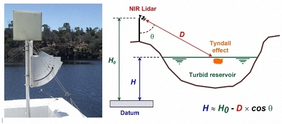
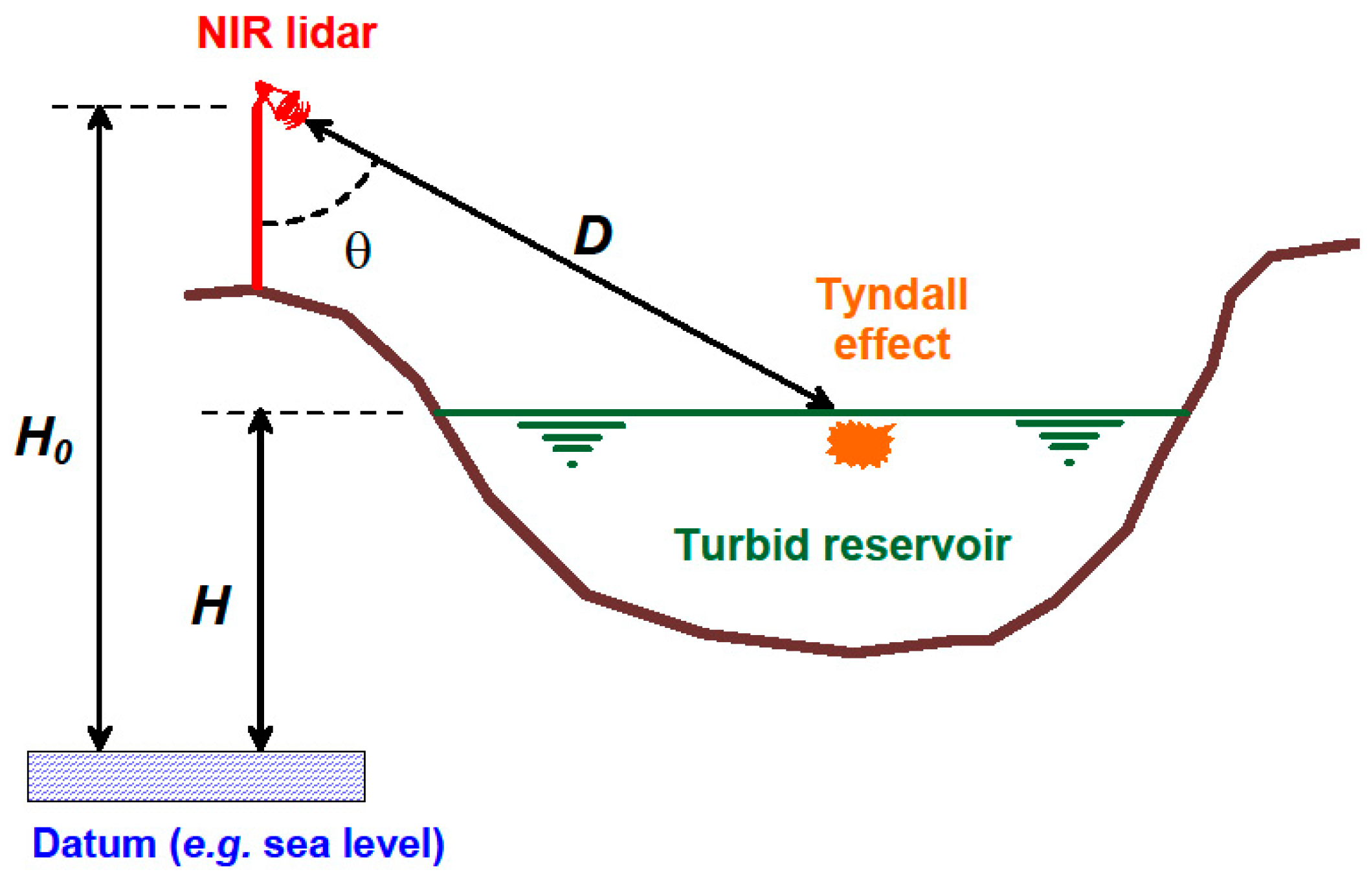
2.2. Fundamentals of the Proposed Technique

Unlike the classical technique that uses a Lidar to measure distance to the water surface, the proposed technique to monitor the stage in turbid water-bodies [1,2] consists of installing the Lidar on a bank and orienting it so that it points at the water surface with a large incidence angle (between ≈ 30° and 70°). With this configuration, a laser pulse sent by the Lidar is reflected specularly by the water surface in such a way that it will not return directly towards the instrument. However, the technique assumes that, some amount of the laser pulse will penetrate (through refraction) into water and will be then partly backscattered (due to the Tyndall effect) by suspended particles that are slightly below the water surface. If so, the stage can be estimated as (Figure 1):
H   =   H 0     D   ×   cos ( θ )
where H (m) is the stage, H0 (m) is the height of the laser above a reference level (datum), D (m) is the distance measured by the laser and θ (°) is the laser incidence angle. In theory, both parameters H0 and cos(θ) can be directly measured; this was done during the laboratory tests described below (Section 3.2), to demonstrate the empiricism of the proposed technique (as explained in the next section).

2.3. Empiricism of the Proposed Technique

A Lidar inclined with a large incidence angle will not measure the distance to the water surface (unless there are flat floating objects), but rather a greater distance due to the penetration of the laser beam into the water. This situation is known as the “surface uncertainty problem” in Airborne Lidar Bathymetry (ALB) (at least, for referring to the difficulty of detecting a water surface with an inclined green Lidar) [10,12]. However, in practice, a near-infrared (i.e., a wavelength strongly absorbed by water if compared to other Lidar wavelengths), eye-safe and narrow-beam Lidar should not be able to detect particles deeper than a few decimeters below a clear water surface [4,10,11], and probably much less in turbid water [7,9,10,13]. Therefore, there is no guarantee that an inclined near-infrared Lidar will always detect particles suspended in water. However, if it does, as expected in the case of turbid water bodies, it should detect those that are rather close to the surface.
The theoretical description of how a laser pulse penetrates into water and is scattered by a cloud of suspended particles is complicated and still not fully satisfactory [2,9,13,14]. No attempt was made to describe this phenomenon known as “volume scattering” during the experimental study described herein. Equation (1) was used empirically during the field experiment, that is, both parameters H0 and cos(θ) were adjusted through a simple calibration. Therefore, and strictly speaking, the present form of the proposed technique does not provide a stage “measurement” but rather a stage “surrogate”. However, a few field [3] and laboratory [6,7] observations suggest that for a given Lidar configuration (which includes the laser wavelength, power and distance) and water turbidity, it can be roughly assumed that the emitted laser pulses penetrate through water up to a constant distance (please, note that such a distance must be seen as an effective property). If so, the bias in the stage estimation can be simply deduced as [4] (please, note that the Lidar “ignores” that its beam is refracted and travels slower into water):
Δ H   =   n w   ×   Δ D 0   × cos ( θ )
where ∆H (m) is the stage underestimation, ∆D0 (m) is the effective distance of penetration of the laser pulses into water and nw is the water refractive index relative to the air (=1.328 for near-infrared). Therefore, the formula suggests that the stage underestimation should be constant for a given Lidar incidence angle. In the case of the commercial Lidar used during this study, this assumption will be verified through laboratory tests.

3. Materials and Methods

3.1. The Test Lidar

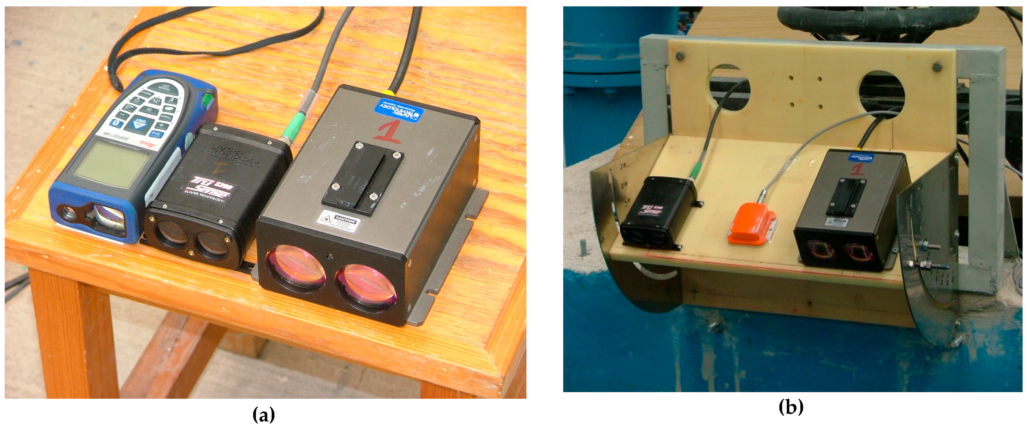
3.1.1. Lidar Selection

To evaluate the proposed technique, commercial Lidar with the following features have been looked for: near-infrared laser (λ = 905 nm), safe-eye (class 1M, which implies a very low laser power), not very expensive instrument (<3000 USD) and serial port (to connect to a datalogger). Of course, these Lidar have been designed to measure the distance to a diffuse target, not for the application considered during this study. In this context, preliminary tests found that some commercial Lidar instruments do not detect a turbid water (sub-) surface as well as others. Although unexplained (due to manufacturing secrets), it seems that the least expensive Lidar instruments perform better than others with similar features [7]. As a matter of fact, tests by Tamari et al. [1] of two models of the same brand (Optech Inc., Vaughan, ON, Canada) found that the “3100-SR Watchman” (firmware 35-AWLX-2.0) provides better results than the more expensive ”Sentry SR“ (firmware SR-V2.8). Similarly, two models by another brand (Laser Technology Inc., Centennial, CO, USA) were tested during this study (Figure 2a,b), finding that the “TruSense S200” (firmware 1.11.4) provided better results than the more expensive “ULS” (firmware 1.0.5). Therefore, only the results obtained with the “TruSense S200” [15] are reported below.

3.1.2. Lidar Configuration and Output

Unlike the simplest Lidar (handheld laser rangefinders), the test instrument [15] comes with a few options to attempt detect a target under non-ideal conditions (i.e., when translucent objects are in front of the target, which can happen in the field when rain, fog, dust or mosquitoes are present). Thus, the test Lidar can measure a distance with three modes, which are well-known in ALB (at least, when analyzing the bottom returns of a green Lidar) as [10]: “first pulse”, “strongest pulse” and “last pulse”. These three Lidar modes of operation were sequentially used by the present study (unlike Tamari et al. [1] who could only use one mode).
The Lidar was programmed to attempt to take one distance data every 1 min. during laboratory testing and every 10 min. during the field experiment. Each attempt to measure distance consisted of a burst of 12 laser pulses (the default value according to the manufacturer) and, in the case of a failed measurement, the Lidar was allowed to try again until reaching a maximum number of 16 attempts. It is worth noting that the Lidar was always left to take distance data freely (unsupervised way), that is, regardless of what was measured before and of what could be considered a priori as realistic.
In addition to each measured distance value, the test Lidar returns a “signal strength” value. Basically, this is an integer (I) which increases from 1 to 4 as the intensity of the laser pulses backscattered to the Lidar detector is higher (according to the manufacturer [15]). Assuming that the signal strength depends mostly of the target reflectance (for a given Lidar configuration), its value was used to analyze the raw Lidar data (it must be recognized that the test instrument also returns another signal strength value (J) which varies between 0 and 1999, but its meaning is unfortunately unclear, due to the lack of information from the manufacturer in spite of a personal request for explanation).

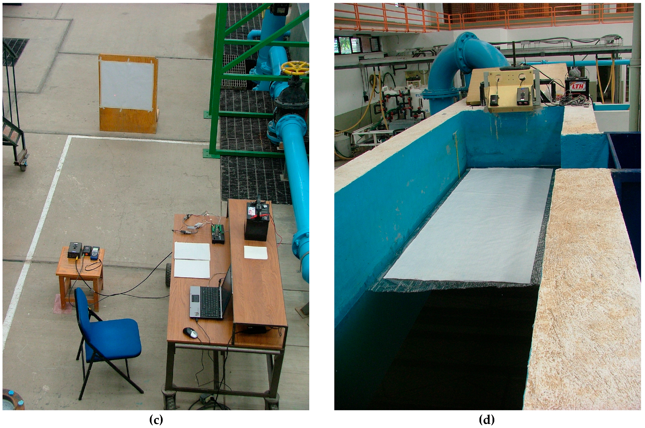
3.2. Laboratory Testing

3.2.1. Preliminary Check and Preparation of Turbid Water

According to its manufacturer [15], the “TruSense S200” Lidar can measure distances to a diffuse target (which is the purpose for which the instrument has been designed) from 0.5 to ≈ 750 m with an uncertainty of ±40 mm. However, as with many others, the manufacturer does report the level of confidence associated with this uncertainty. Therefore, the ability of the Lidar to measure the distance to a diffuse surface (Figure 2c) was first verified in the laboratory (for distances between 0.5 and 50 m): when comparing it to a handheld laser rangefinder (“Disto A6”, Leica Geosystems, Heerbrugg, Switzerland), which is much more accurate for this type of application [16], the “TruSense S200” was found to underestimate distance by ≈ 30 mm (two Lidar units were systematically tested with the “first pulse”, “strongest pulse” and “last pulse” modes); however, after correcting for this bias, the Lidar uncertainty was found to be better than ±40 mm (p = 0.95). In the following, the raw distance data provided by the test Lidar have been systematically corrected for this bias.
Once checked the ability of the test Lidar to measure distances to a diffuse target, two series of tests were then performed using a water tank to investigate the ability of the Lidar to estimate the stage in turbid water. To prepare the turbid water, solid particles were mixed into tap water. Three types of solid particles were successively used: (1) a silty material known as Tepetate (the Mexican name for a type of volcanic-ash soil); (2) a finer material known as Andosol (another type of volcanic-ash soil, typical in the area of the Cointzio reservoir where the Lidar was further tested); and (3) the same Andosol material artificially dispersed into water by adding a detergent (≈ 0.8 g/L of sodium hexametaphosphate). Before starting each test, special care was taken to remove all the floating matter (such as small flocculated aggregates and organic matter). During the tests, the water turbidity was assessed using a Secchi disk, which is a black-and-white disc that is lowered into the water by a graduated line. The depth of visual disappearance of the disk—the so-called “Secchi depth” (ZD, m)—is indeed a simple but useful index of water clarity [17]. This Secchi depth was between ≈ 0.4 and 0.6 m at the beginning of each test performed on the water tank, which corresponds to extremely turbid water.

3.2.2. Effects of the Lidar Incidence Angle and Water Transparency

A first series of test was performed on the water tank (≈2.6 m deep, 4.5 m long and 0.9 m wide) to investigate the ability of the Lidar to detect the (sub-) surface of extremely turbid water (Secchi depth ≈ 0.6 m) as a function of the instrument incidence angle, which ranged from ≈ 0° (specular condition) to 70° (Figure 2b). The true height of the Lidar above the tank bottom (H0, measured with an uncertainty of a few mm) and the true incidence angle (θ, measured with a tolerance <1° using an electronic inclinometer: “MTi”, Xsens Technologies, Enschede, Netherlands) were used to convert the measured distance data (D) into stage estimates (H) according to Equation (1) (with two simple geometrical corrections also made to account for the Lidar length and height). As a reference, the distance to a diffuse surface (white cloth sheet) temporarily placed above the water surface (Figure 2d) was also measured and converted into stage data.
Another series of tests were performed on the water tank to investigate the ability of the Lidar mounted with a large incidence angle (≈60°) to monitor the stage over a few days, as water was getting less turbid (due to the sedimentation of suspended particles). During these tests, a slow decrease in the stage was also simulated by opening a drainage valve at the tank bottom and the stage was manually checked at times (using a graduated scale). A submersible pressure transducer (“DCX-16VG (50 kPa)”, Keller, Newports News, VA, USA) was used as a reference to monitor the stage, and as discussed previously [1], this instrument was expected to estimate the stage with an uncertainty better than ±10 mm (p = 0.95) in artificially-prepared turbid waters.

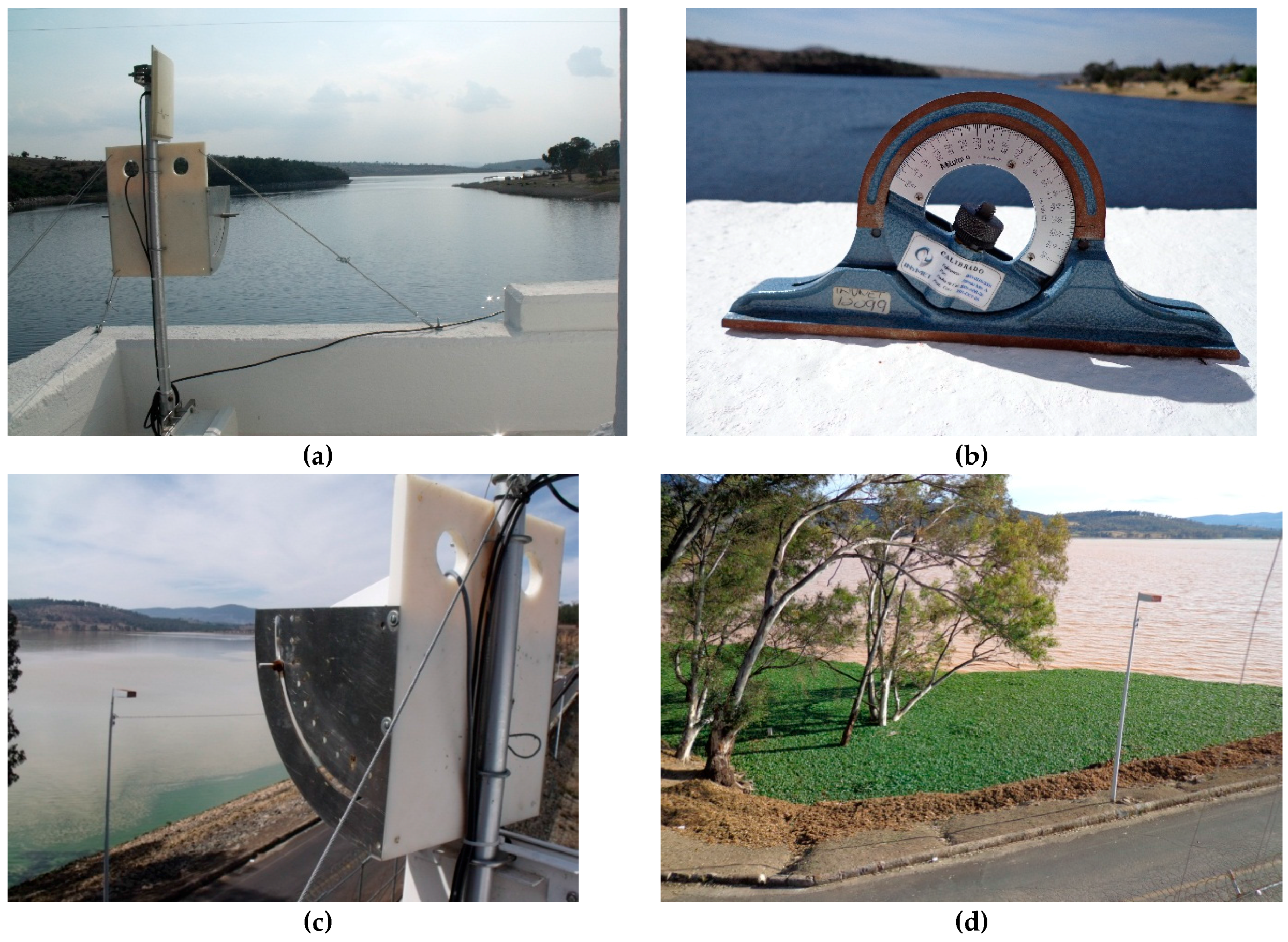
3.3. Field Experiment

3.3.1. Site Selection

To assess the ability of the proposed technique to monitor the stage under field conditions, a three-years experiment was performed (May 2012–July 2015) in two turbid reservoirs from the central part of Mexico (Figure 3): Cointzio (Michoacán state; 19°37′51″N–101°15′29″W) which is extremely turbid due to the presence of highly erodible soils and Valsequillo (Puebla state; 18°54′45″N–98°06′32″W) which is very turbid due to the presence of wastewater.

3.3.2. Instrumentation

A “TruSense S200” Lidar unit was installed on the bank of each reservoir, mounted on a small mast and connected to a datalogger (“CR-1000”, Campbell Scientific, Logan, UT, USA). The unit at Cointzio was located at an elevation of ≈ 13 m above the Ordinary High Water Level (OHWL) and the unit at Valsequillo was located at an elevation of ≈ 6 m above the OHWL. Each Lidar was pointing at the water surface with a large incidence angle; specifically, θ = 71.0° at Cointzio (measured before October 2013), and θ = 62.0° (before 2014) or 63.5° (after 2014) at Valsequillo, according to the measurements provided by both an “MTi” electronic inclinometer and a bubble inclinometer (Figure 3b). The Lidar incidence angle at Valsequillo was not the same before and after 2014 probably because the plate supporting the Lidar may have moved slightly when the unit had to be replaced due to damage by a short-circuit in the datalogger. In addition, a preliminary analysis of the raw data obtained at Cointzio suggests that the Lidar incidence angle also changed slightly after October 2013, which was probably due to the loosening of the cables used to hold the mast that supported the Lidar (a problem that could be avoided in the future by using a more rigid support for the Lidar); in this case, it was decided to fit this new incidence angle using the calibration procedure described below (Section 4.2.1).
Once installed in the field, both Lidar instruments were programmed to attempt to take distance measurements every 10 min. As mentioned previously, the distance was taken with three different modes and the signal strength associated with each measurement was recorded. In parallel, the stage in both reservoirs (Href, m) was manually measured daily using a limnimetric scale (referenced to the sea level); these stage data (taken with an uncertainty of ≈±0.01 m (p = 0.95)) have been used as a reference to assess the ability of the proposed Lidar technique to provide stage estimates.
During the field experiment, the Secchi depth (ZD, m) was measured once a week, to assess the water turbidity. The precipitation (P, mm/d) was also manually measured, to see if it affects the Lidar measurements; in addition, it was thought that the reservoir turbidity would increase at the beginning of every rainy season, due to an enhanced soil erosion. No attention was paid to the wind speed, because the “glint noise” due to water agitation was expected to be small in case of a conventional Lidar inclined with a large incidence angle (as said in Section 2.1 and as discussed in Section 4.3.2); it could be also argued that a strong wind should increase the number of suspended particles below a water surface (which would be a positive effect for the proposed technique), but this is out of the scope of this study.

4. Results and Discussion

4.1. Laboratory Results

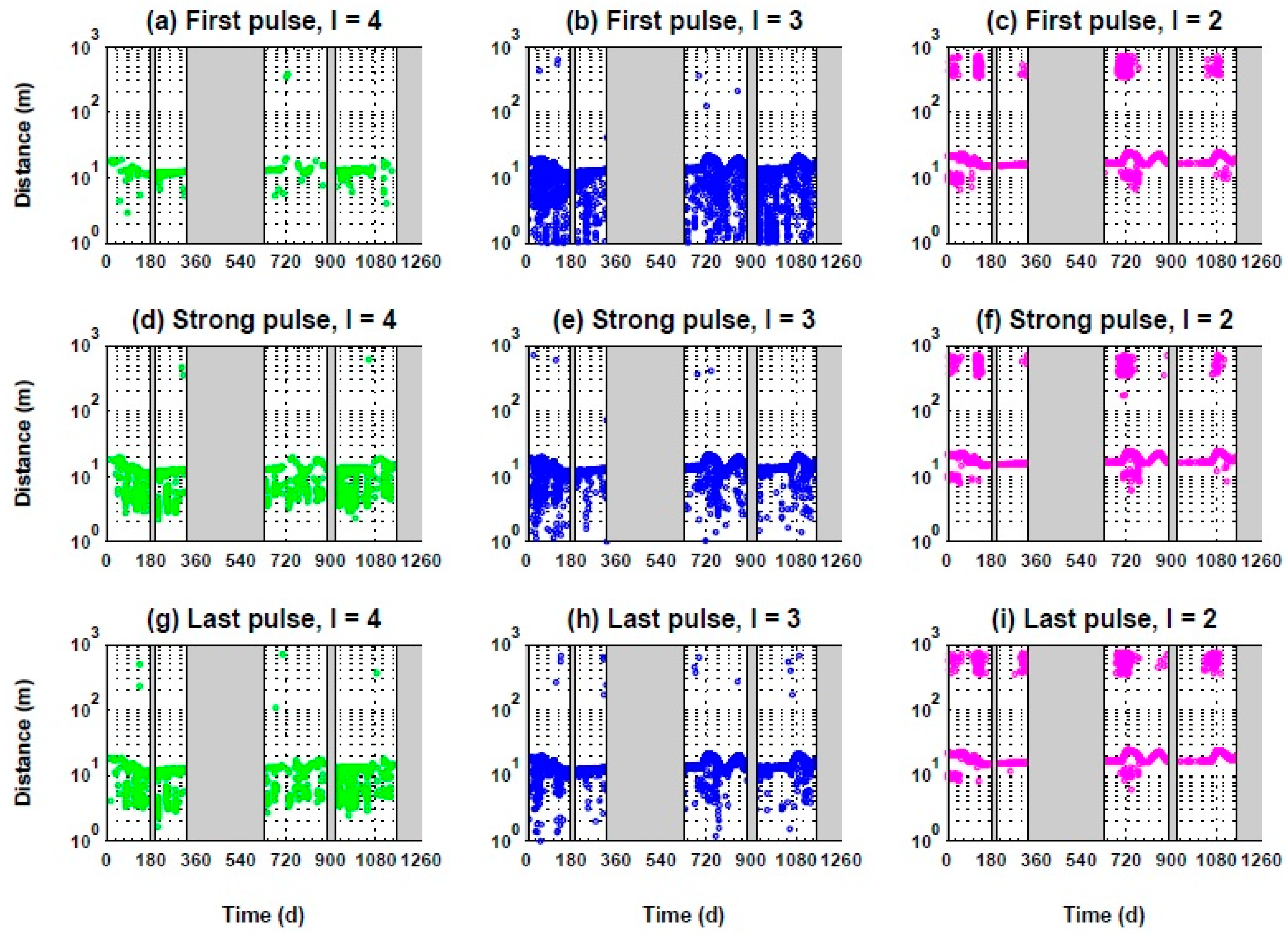
4.1.1. Raw-Data Filtering

When mounting the “TruSense S200” Lidar with a large incidence angle over a tank filled with turbid water, some incoherent and erratic distance data were recorded on occasion. Most of these were much higher (by several metres) than the distance to the water surface and were associated with a low signal strength (I = 2), which was interpreted as the result of a specular reflection of the Lidar’s laser beam at the water surface followed by a diffuse reflection on a wall inside the laboratory.
By trial and error, a simple empirical rule was found to filter the raw distance data: a high signal strength (I = 4) was interpreted as the direct detection of a diffuse object, a moderate signal strength (I = 3) was interpreted as the detection of a turbid water (sub-) surface, and a low signal strength (I = 2) was not related to the detection of any desired target. Therefore, the only data kept were the raw data associated with a high signal strength (I = 4) during tests with the Lidar pointing at a diffuse surface, and the only raw data used to estimate stage values (according to Equation (1)) were those associated with a moderate signal strength (I = 3) during tests with the Lidar pointing at a water surface. In addition, and as expected under ideal conditions (i.e., with no rain, fog or dust) [15], the test Lidar was found to provide more coherent data when configured in the “first pulse” or “strongest pulse” mode, as opposed to the “last pulse” mode.

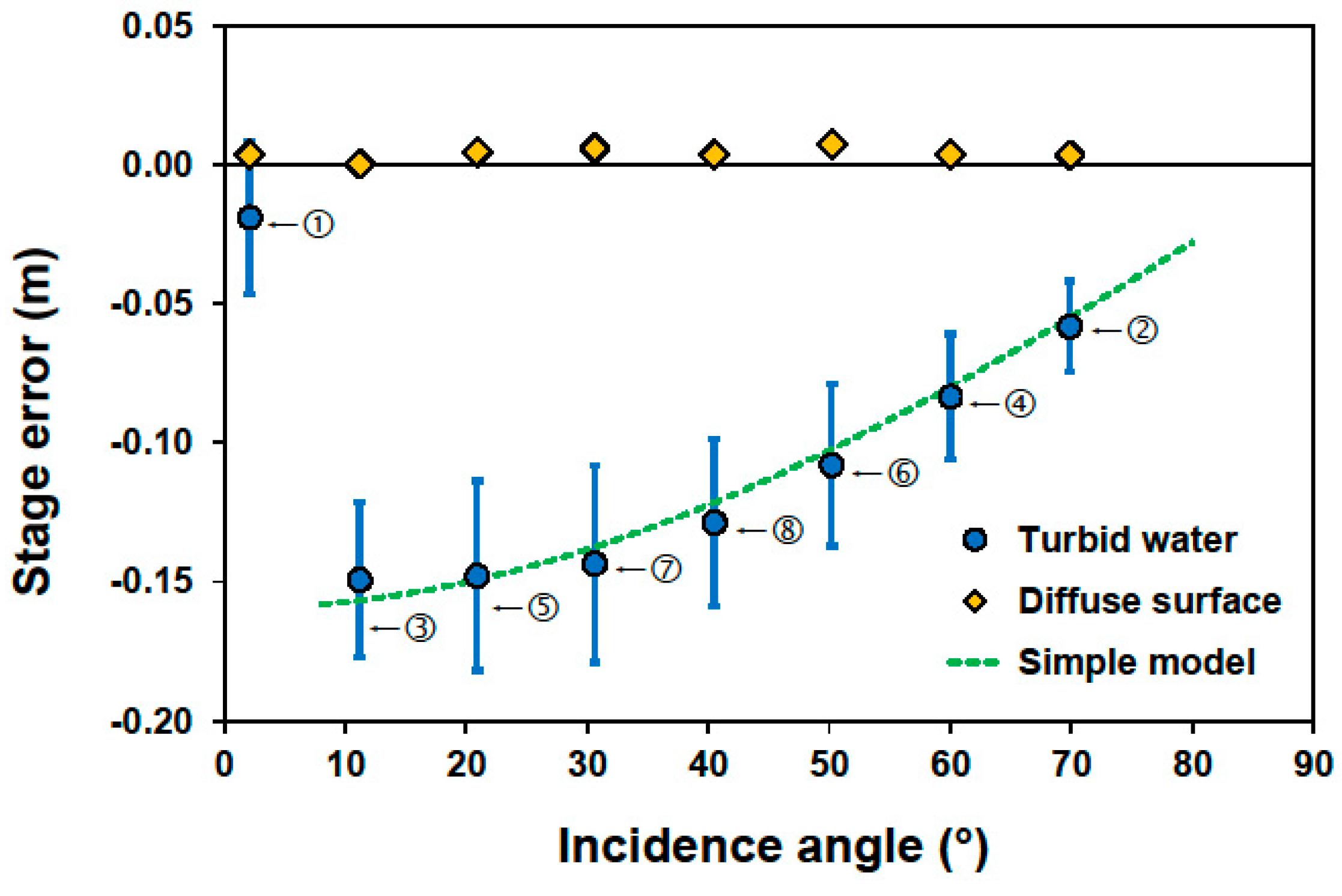
4.1.2. Effects of the Lidar Incidence Angle and Water Transparency
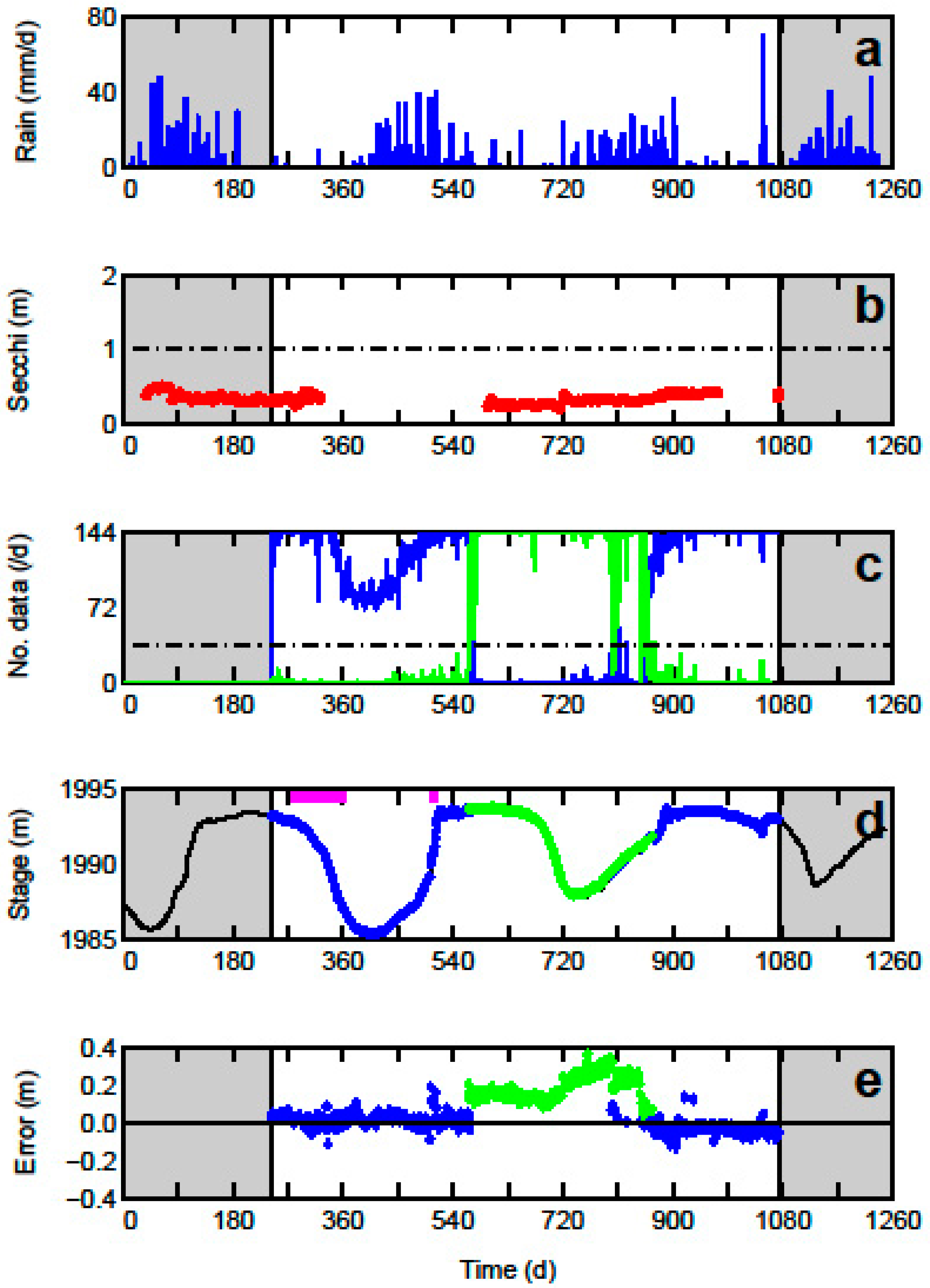
Figure 4 shows an example of how the “TruSense S200” Lidar mounted with different incidence angles responds when it points at a target. First, it was checked that the Lidar had no difficulty to estimate the distance to a thin diffuse surface placed above the water and therefore to accurately estimate the stage like this (error < 10 mm for the mean of ≈ 30 replicates). Then, it was checked that the Lidar mounted with a small incidence angle (θ ≈ 0°) over a water surface can estimate the stage with a rather low error (<20 mm), as was expected since this is the conventional way to use a Lidar to monitor the stage in water bodies. Finally, the Lidar mounted with a large incidence angle (θ > 10°) over an extremely turbid water surface (Secchi depth ≈ 0.6 m) was found to significantly underestimate the stage, which is consistent with the idea that the laser pulses emitted by the instrument penetrate into the water and are then backscattered by suspended particles.
In addition, the Lidar pointing at a turbid water surface with a large incidence angle was found to underestimate the stage with a magnitude which depends on the incidence angle: from −0.15 to −0.06 m as the incidence angle increases from 10° to 70° in the example shown at Figure 4 (similar results were obtained when testing the Lidar in each mode of operation and with the three different materials used to prepare the turbid water). In this case, the very simple model of light penetration into water (Equation (2)) was found to satisfactorily describe the results when the distance of penetration of the laser pulses into water (∆D0) was fitted to ≈ 0.12 m; this value was of the same magnitude, although twice larger, as what was obtained during another laboratory study performed with a different commercial Lidar (according to Figure 7 in [6]). However, the uncertainty in the stage estimations by the inclined Lidar pointing at a turbid water surface was larger -up to five times- than the uncertainty of the Lidar pointing at a diffusive surface: this could be due to a variability in the effective distance of penetration of the laser pulses into water (∆D0) from one replicate to the other (mainly due to a varying absorption and scattering of the laser pulses by turbid water). It is also worth noting that the stage estimations were tending to be less noisy at large incidence angles, which could be due to a combination of two phenomena: as the Lidar incidence angle increases, the vertical projection of the measured distance is less sensitive to the distance uncertainty and the depth of penetration of the Lidar beam decreases. Nevertheless, the test Lidar was virtually unable to detect a water sub-surface when its incidence angle was larger than ≈ 75°.
Figure 5 shows an example of how the “TruSense S200” Lidar responds when it points with a large incidence angle at a turbid water surface. Again, it shows that the Lidar underestimates the stage by a nearly constant value (for a given incidence angle) when its real position above the water surface and incidence angle are used (i.e., H0 and θ in Equation (1)). By trial and error, the lowest turbidity for which the test Lidar can detect a water (sub-) surface was investigated: according to the laboratory tests, it was equivalent to a Secchi depth of ≈ 1.0 m (e.g., Figure 5) when the Lidar was configured in the “first pulse” or “strongest pulse” mode. However, this result was obtained under ideal conditions and thus must be considered carefully. For instance, it was observed that the Lidar sometimes provides erratic distance data even when the water is very turbid (e.g., see Figure 5 at times ≈ 21 and 90 h), which could be due to an effect of ambient conditions (light or temperature), since the erratic data were usually obtained at the end of the afternoon. Therefore, and as discussed below, the lowest turbidity for which the test Lidar can detect a water (sub-) surface must also be investigated under non-ideal field conditions (with special interest on possible effect of rain and sun-light).

4.2. Field Results

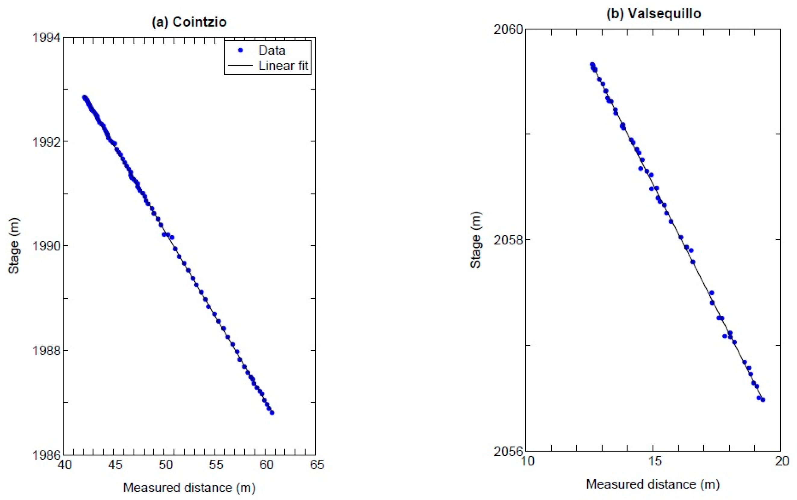
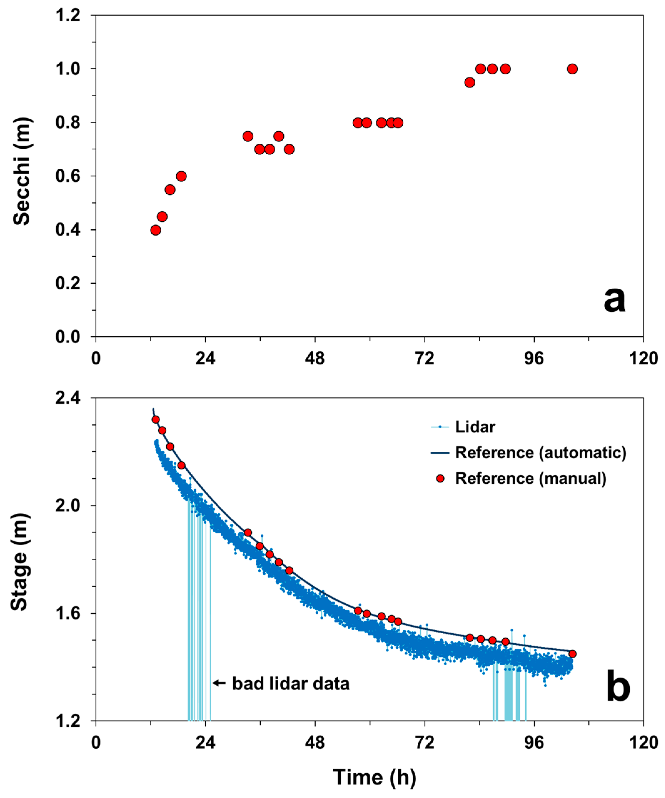
4.2.1. Raw-Data Filtering and Field Calibration

Similar to what was observed during the laboratory tests and as reported by a previous study [1], the raw distance data recorded by the test Lidar were quite erratic during the field experiment performed in two turbid reservoirs (Figure 6 and Figure 7). However, and in agreement with the results obtained during laboratory tests, it was empirically found that these data can be filtered according to the intensity of the received signal (I). A high signal strength (I = 4) was usually consistent with the detection of objects floating on the water surface, unless an opaque object (as might be a bird) had passed in front of the Lidar or the water was extremely turbid (Secchi depth less than ≈ 0.5 m); as shown below, the detection of floating objects occurred mostly at Cointzio due to a patch of water hyacinth (Eichhornia crassipes) which remained in front of the Lidar’s line-of sight for one year (Figure 3d). Meanwhile, a moderate signal strength (I = 3) was usually consistent with the detection of a water (sub-) surface, unless a translucent object (such as a cloud of mosquitoes or a strong rain) had passed in front of the Lidar. In addition, a lower signal strength (I = 2) was related to the detection of other less obvious features (see Appendix A).
Considering that a received signal having a moderate intensity (I = 3) was usually related to the detection of a turbid water (sub-) surface, the “strong pulse” mode was found to be the best configuration for the test Lidar: it indeed provided more distance data associated with a moderate signal strength, both at Cointzio (Figure 6e) and Valsequillo (Figure 7e). Therefore, only the raw Lidar data obtained with the “strongest pulse” mode were used to estimate the stage data. However, these data were still erratic. In addition, they presented small daily oscillations, which are still difficult to explain (see Appendix B). Therefore, it was decided to regroup and filter the raw Lidar data on a daily basis.
By trial and error, a simple algorithm was found and used to extract the raw Lidar data (obtained in the “strongest pulse” mode) that were likely associated with the detection of a water (sub-) surface. This algorithm consists of: (1) removing distance data smaller than 1 m (which occurred at times and were obviously due to a human or a bird being in front of the Lidar); (2) keeping only the “good” distance data, i.e., those associated with a moderate signal strength (I = 3); (3) grouping these data per day and computing their median; (4) keeping only the medians that had been computed with a sufficient number of “good” data (ngood ≥ 36, which corresponds to at least 25% of the 144 attempts to measure a distance per day), otherwise (5) considering the Lidar to have been unable to estimate the stage for a given day. The same algorithm was also used to extract raw Lidar data that were likely associated with the detection of floating objects: in this case, the distance data associated with a high signal strength (I = 4) were used in step (2). The proposed algorithm is quite robust, even though it can only provide one stage estimate per day. As a matter of fact, it attempts to estimate each stage data independently of what had been estimated previously. In addition, and contrary to findings by Mandlburger et al. [12], its performances were not found to be significantly different when computing the third (or the first) quartile of the raw distance data instead of the median during step (3).
For the case of the field experiment, Equation (1) was used empirically to estimate stage data based on the Lidar distance measurements; that is, both parameters H0 and cos(θ) were adjusted through calibration. This calibration was performed according to the following algorithm: (1) select a period corresponding to the filling or emptying of the reservoir (≈3 months in practice); (2) filter the raw Lidar data according to the previous algorithm (for a moderate signal strength: I = 3); and (3) perform a linear regression on the experimental relationship between the filtered Lidar distance data (D) and the stage data recorded for the same days, according to a limnimetric scale (Href). As shown in Figure 8, the calibration results were satisfactory, with a standard deviation of the residuals smaller than 30 mm (i.e., close to the Lidar uncertainty when operating under ideal conditions; see Section 3.2.1). Based on the slope of the calibration lines, the Lidar incidence angle (θ) was estimated to be 70.99° (before October 2013) or 71.17° (after October 2013) at Cointzio and 61.75° (before 2014) or 62.28° (after 2014) at Valsequillo, which is consistent with the direct measurements obtained with an inclinometer (see Section 3.3.2). In addition, similar estimates of H0 (difference < 12 mm) were obtained for both calibrations performed at Valsequillo (before and after 2014).

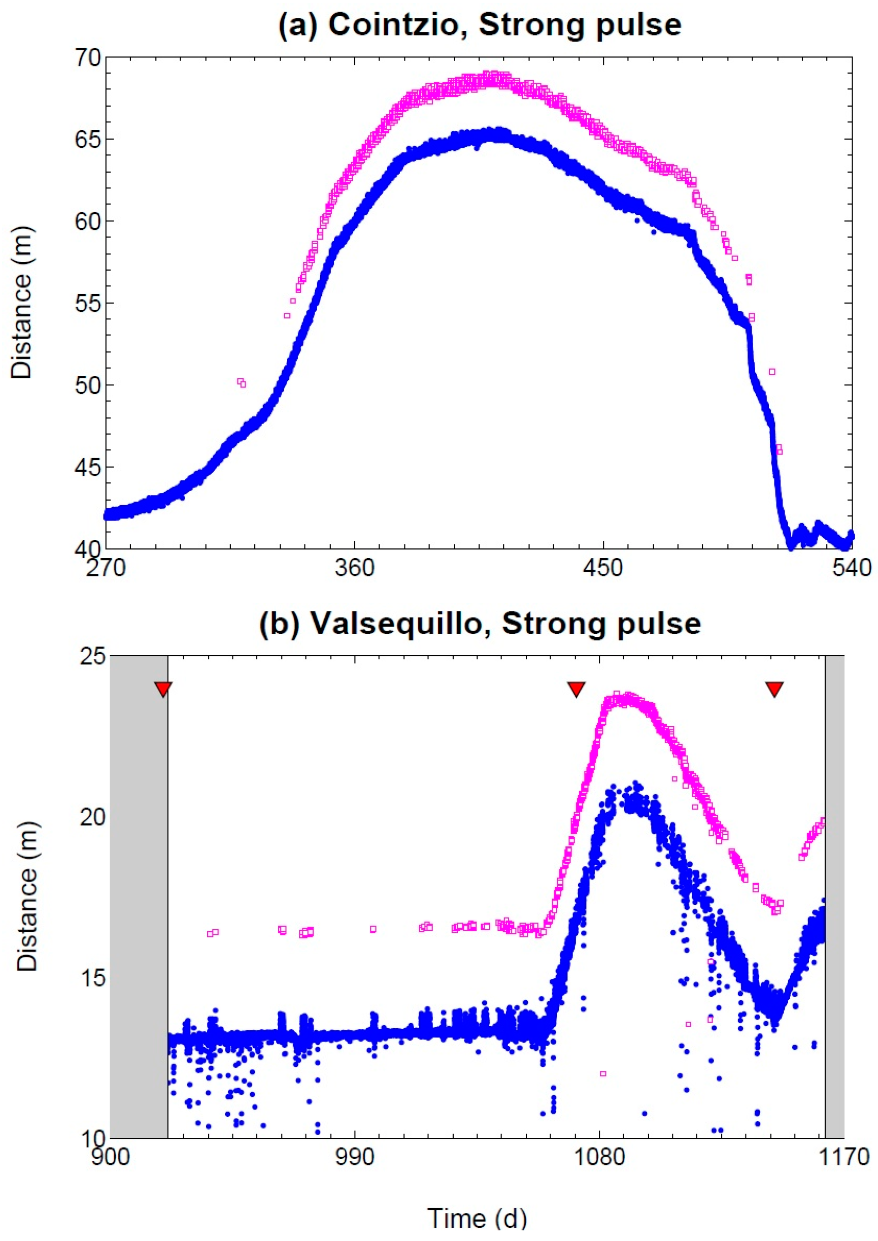
4.2.2. Stage Estimation

After estimating both parameters H0 and cos(θ) through calibration, the filtered Lidar distance data were converted into stage estimates and compared to the reference values on a daily basis (to this end, the reference data were linearly interpolated for the times associated with the Lidar data). The main results from the long-term assessment of the technique proposed to monitor the stage in turbid reservoirs are shown in Figure 9 for Cointzio and Figure 10 for Valsequillo (in both cases, some Lidar data were unfortunately lost due to electrical failures of the datalogging systems).
In the case of the Cointzio reservoir, the water was extremely turbid all the time, with a Secchi depth of ≈ 0.4 m (Figure 9b). Under these conditions, the proposed technique had no difficulty to estimate a stage value every day (Figure 9c,d). When the Lidar was detecting a free water (sub-) surface (associated with a received signal having a moderate intensity: I = 3), these estimates were consistent with the reference data within ±0.085 m (p = 0.95) (see blue points on Figure 9d). However, the results obtained at Cointzio suggest that the Lidar had also detected floating objects (associated with a received signal having a high intensity: I = 4) for one year (see green points on Figure 9d,e), which is consistent with the fact that a patch of water hyacinth remained in front of the Lidar’s line-of-sight during the same period (Figure 3d); under these conditions, there was more discrepancy between the stage data estimated with the proposed technique and the reference data (see green points on Figure 9e). Obviously, the presence of (opaque) floating objects will produce a bias when trying to estimate the stage with a non-contact technique, and this bias will increase as the objects are higher (up to ≈ 0.35 m for the water hyacinth detected at Cointzio). Nevertheless, the proposed technique makes it possible to detect this problem rather easily.
In case of the Valsequillo reservoir, the water was less turbid: the Secchi depth was varying between 0.4 and 2.1 m (Figure 10b), with no clear relationship with the precipitation (Figure 10a); the lack of correlation between Secchi depth and precipitation was unexpected, but is out of the scope of this study. Under these conditions, the proposed technique could not provide a stage estimate every day (Figure 10c,d). However, it usually did when the Secchi depth was <1.0 m, which is consistent with the laboratory results (Section 4.1.2). This suggests that ambient conditions (such as rain, sun-light and air temperature) do not greatly affect the response of the test Lidar when the water is very turbid. When stage data at Valsequillo could be estimated with the proposed technique, they were consistent with the reference data within ±0.078 m (p = 0.95) (Figure 10e), which is similar to the results obtained at the Cointzio reservoir (of course, our data analysis slightly overestimates the uncertainty of the proposed technique since it includes the uncertainty of the reference technique, which was of ≈±0.01 m (p = 0.95)).
However, it must be recognized that the test Lidar had some difficulties to detect the water (sub-) surface at the end of the experiment performed at Valsequillo (see Figure 10c at time ≈ 1080 days) even though the water was very turbid (see Figure 10b): this occurred during a period when the stage was changing rather rapidly (see Figure 10d). In fact, the test Lidar also had some difficulties to detect the water (sub-) surface during others periods with rather rapid stage changes both at Valsequillo (e.g., see Figure 10c,d at time ≈ 720 days) and Cointzio (e.g., see Figure 9c,d at time ≈ 400 days). Was this due to a change in the turbidity profile below the water surface while the stage was changing? Further studies are needed to answer this question.
A summary of the stage estimations obtained using the proposed technique during the field experiment is shown in Table 1. Unlike Cointzio, the conditions at Valsequillo were not favorable to implementing the technique; nevertheless, the experiment performed at Valsequillo was useful to define the scope of the technique.
.

4.3. Discussion

4.3.1. Reliability of the Proposed Technique for Stage Monitoring in Turbid Reservoirs

This study shows that the proposed technique for monitoring the stage of turbid water bodies can be applied using simple and cheap Lidar instruments. However, some available models do not work as well as others (Section 3.1.1): although unexplained (due to manufacturer secrets), this can be rapidly checked in a water tank.
This study also shows (Section 4.1.1 and Section 4.2.1) that among the three available configuration modes of the test Lidar, the “strongest pulse” mode is the best one for detecting a water (sub-) surface. However, the other two modes, especially the “first pulse” mode, can be useful to corroborate the detection of a water (sub-) surface. More importantly, the signal strength of the Lidar returns was found to be a crucial criterion to know if a water (sub-) surface has been detected.
It was verified in the laboratory (Section 4.1.2) that the effective distance of penetration of the test Lidar pulses into water is rather small and nearly constant (≈0.12 m), provided that the water is very turbid (Secchi depth smaller than ≈ 1.0 m). As far as we know, only Streicher et al. [6] have previously verified this idea with a Lidar inclined at different incidence angles.
The fact that an inclined Lidar can detect suspended particles into water at a nearly constant depth (for a given Lidar incidence angle) makes it possible to apply the proposed technique for monitoring the stage of turbid reservoirs, as proposed by Tamari et al. [1] and as verified during the long-term experiment described in this study (Section 4.2.2).
Of course, the main disadvantage of the proposed technique is that it only works for turbid water. Until now, few laboratory [4,5,6,7] and field [1] studies have shown that some commercial near-infrared Lidar instruments can easily detect the (sub-) surface of extremely turbid waters, i.e., when the turbidity is over ≈ 40 NTU. This is roughly equivalent to a Secchi depth smaller than ≈ 0.5 m and to a suspended sediment concentration (SSC) over ≈ 100 g/m3 (e.g., [17]). In this respect, the present study suggests that the proposed technique can be applied to less (but still very) turbid water (Secchi depth up to ≈ 1.0 m), in which case it could be applied to reservoirs having the following characteristics: dam embankments or lakes surrounded by erodible soils (e.g., [18,19]), shallow lakes exposed to wind (e.g., [20,21]), hypereutrophic or brown-water eutrophic lakes (e.g., [22,23]) and wastewater reservoirs. At least 10% of the reservoirs and lakes over the world are very to extremely turbid (Secchi depth < 1.0 m) [23].
Now, the question arises to know if it is worth considering the proposed technique –in terms of accuracy and easiness of use- for monitoring the stage in turbid reservoirs. Nowadays, conventional techniques can be used to monitor the stage of water bodies with an uncertainty usually better than ±0.01 m (p = 0.95) (e.g., [24]), provided that they have been carefully implemented. In this regard, the present form of the proposed technique is rather inaccurate. Nevertheless, it has some practical advantages, including its easy implementation in a safe place (such as the roof of a building), quick installation (less than 2 h), low maintenance requirements and low equipment costs (the price of the Lidar used in this study was ≈ 1500 USD). Therefore, the technique should be seen as an option when there is no other alternative to monitor the stage.

4.3.2. Other Potential Applications of the Proposed Technique

Another potential application of the technique is to study certain coastal areas, such as estuaries, surf zone and swash zone: as a matter of fact, the water in these areas contains a large amount of suspended solid particles and/or air bubbles (e.g., [2,25,26]). In this context, it is worth noting that a growing number of experimental studies are showing the usefulness of commercial Terrestrial Lidar Scanning (TLS) systems to map the water surface of some rivers [3,4] and coastal areas [25,26]. Although this technique appears to be similar to the one described in this study, it is not explicitly based on the same physical principle: as a matter of fact, studies suggest that TLS systems are mostly able to detect water surface due to “glint noise” after a very large number of attempts and provided that the surface is agitated enough. It is recognized that they can also detect the water surface due to the diffuse reflection by foam or whitecaps, as well as the sub-surface due to the Tyndall effect (which is the physical principle considered in this study); however, and as far as we know, no attempt has been made until now to distinguish water sub-surface detection from water surface detection during a monitoring campaign performed using a TLS system.
The proposed technique could also be used to monitor flash floods in rivers: as a matter of fact, the water is usually very turbid during this type of flood [4,27]; in this case, it is worth noting that “glint noise” should only slightly affect the response of a common Lidar pointing at a water surface with an incidence angle between ≈ 30° and 70°, unless the surface agitation is extreme [2,9].
Until recently, the inclined Lidar technique has been used only on rare occasions. This could be due to practical as well as theoretical reasons: most water bodies are not very turbid (e.g., [19,24]) and the technique is still empirical because it is difficult to describe volume scattering. However, with the help of Lidar experts (e.g., [2,10,14]) and manufacturers, it is hoped that the versatility (for less turbid water) and accuracy (detection of a turbid layer closer to the water surface) of the technique will improve in the future (for example, by using Lidar that can record a full waveform). Meanwhile, a few experiments performed with simple commercial instruments suggest that the inclined Lidar technique is promising to monitor not only the stage, but also the sub-surface velocity in turbid water bodies. As a matter of fact, if an inclined Lidar detects suspended particles below the water surface, it can potentially determine their velocity relative to the Lidar’s line-of-sight (using the Doppler effect); this would enable estimating the water velocity below the surface (including, hopefully, vertical water velocity profiles): an idea [1] patented almost twenty years ago [28] but not yet officially tested (please, note that the setup considered in this study is different from that of conventional Laser Doppler Velocimetry (LDV), where the laser beam is focused with a lens on a small water volume).

5. Conclusions

This experimental study is based on the fact that a near-infrared Lidar inclined with a large incidence angle (between ≈30° and 70°) can detect suspended particles that are slightly below the water surface, provided that the water is turbid enough (at least, when the Secchi depth is smaller than ≈1.0 m). In this case, the present study demonstrates that a simple terrestrial Lidar can be used to estimate daily stage data in some reservoirs with an uncertainty better than ±0.08 m (p = 0.95). Although the present form of the technique is not very accurate, it uses an inexpensive Lidar (≈1500 USD) that can be easily installed in a safe place (such as the roof of a building). Finally, the proposed technique could be used to monitor not only the stage in turbid reservoirs, but also the stage and the sub-surface velocity in others turbid water bodies, such as some coastal areas (a recent field of application, which still needs more investigations about what is detected by an inclined Lidar) and flooding rivers.

Acknowledgments

Thank you to Rubén Eric de la Cruz Rodríguez, Isaac Villaseñor Cabrera and Martín García Zacarías (Irrigation District 030 “Valsequillo”, Pue.), as well as to León Torres Aguilera and Pedro Larios Paredes (Irrigation District 020 “Morelia-Querendaro”, Mich.) for allowing the field testing. Thank you to Salvador Cortés Tenorio and Cristián Osorio Campos (DISIME S.A. de C.V.) for their help with data acquisition, to Aldo Gutiérrez Arroyo (Université de Rennes) for his comments and to Patricia Navarro Suástegui (CENCA) for her help with the bibliographic search.

Author Contributions

Serge Tamari and Vicente Guerrero-Meza conceived the experiments; Younès Rifad contributed to obtaining and analyzing the laboratory results; Luis Bravo-Inclán and José Javier Sánchez-Chávez contributed to characterizing the water quality and analyzing the field results; Serge Tamari wrote the paper.

Conflicts of Interest

The authors declare no conflict of interest. The trademark of the instruments is mentioned in the paper for identification purposes only; as a matter of fact, instruments from other trademarks but with similar features can be found on the market.

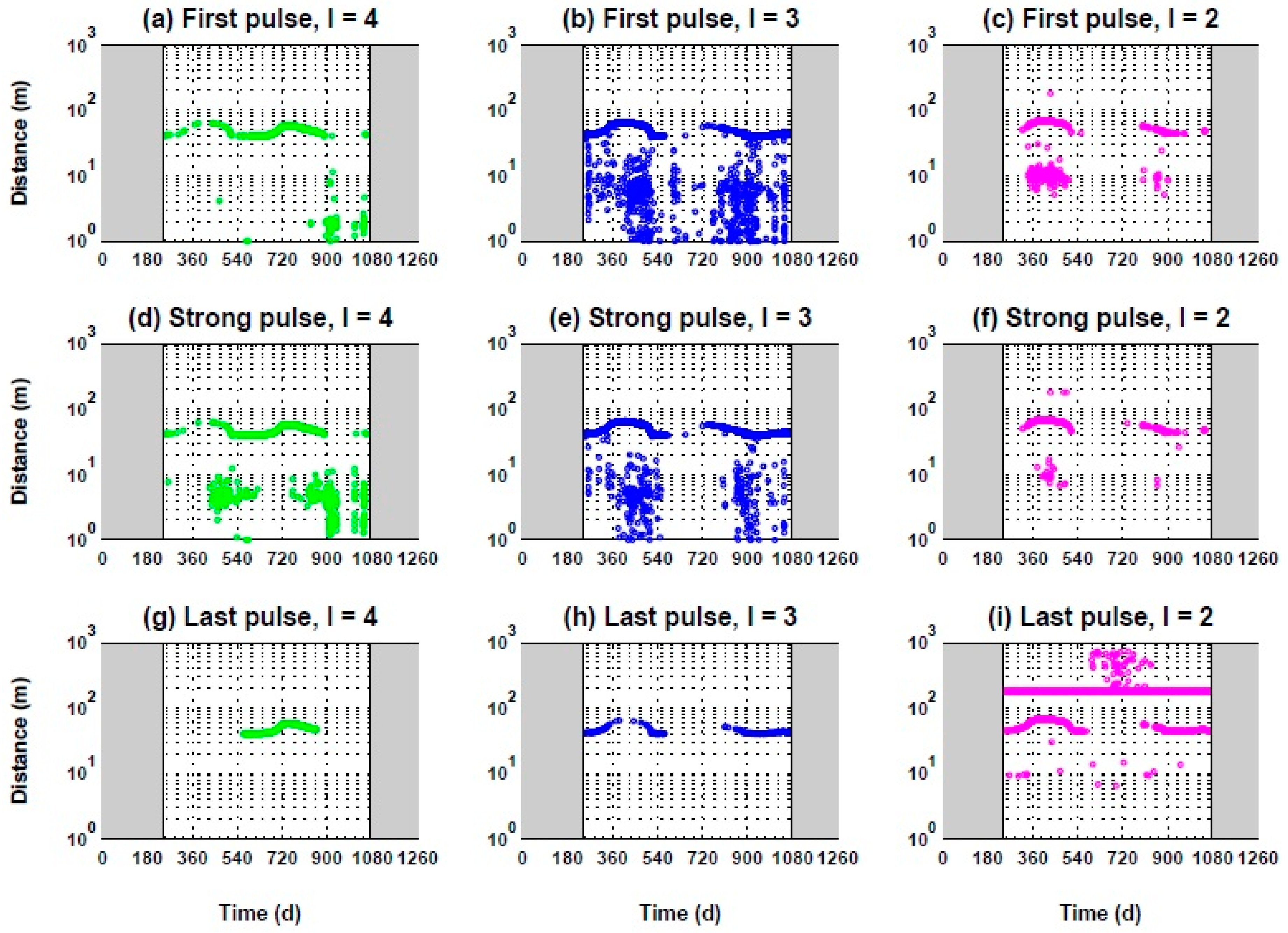
Appendix A—Unexplained Lidar Returns Associated with a Low Signal Strength

When the “TruSense S200” Lidar was tested in the field, the raw Lidar data associated with low signal strength (I = 2) were usually related to the detection of two features. One was an obvious combination of a specular reflection of the laser beam at the water surface followed by a diffuse reflection on a distant solid object; in this case, the measured distance was between 100 and 750 m (e.g., see Figure 6i and Figure 7i). The other and more mysterious feature was the apparent detection of a layer below the water surface: as a matter of fact, by assuming that the raw Lidar data associated with a moderate signal strength (I = 3) were usually related to the detection of a water (sub-) surface (see Section 4.1.1 and Section 4.2.1), some raw Lidar data associated with a low signal strength (I = 2) were overestimating the distance to the water surface by: ∆D ≈ 4.0 m at Cointzio (Figure A1a) and ≈ 3.0 m at Valsequillo (Figure A1b). In this case, a simple optical model based on the Snell-Descartes law suggests that the Lidar was detecting a layer at a depth of: Δ H 0 = [ Δ D / n w ] × 1 [ sin ( θ ) / n w ] 2 , which is 2.1 m for Cointzio and 1.7 m for Valsequillo.
The test Lidar’s apparent detection of a layer at a depth of ≈ 2.0 m below the water surface occurred more often in summer (when a thermocline should be present in the reservoirs studied) and in the afternoon. However, this layer is unlikely to exist since: (1) as far as we know, in practice a near-infrared and low-power Lidar cannot detect suspended particles below a depth of a few decimeters (see Section 2.3); (2) three water column characterizations performed at Valsequillo at different times (November 2014 and April and June 2015; see triangles at Figure A1b) with a multi-parameter probe (“Exo2”, Ysi, Yellow Springs, OH, USA) did not show any obvious stratification at a depth of ≈ 1.7 m (in terms of water temperature, oxygen demand, turbidity and chlorophyll-a concentration), and above all, (3) the same feature was observed later with the test Lidar pointing at a turbid river (the Amacuzac River [27]) when the stage was less than 1.0 metre. Therefore, the Lidar data suggesting the apparent detection of a layer below the water surface were likely to be due to a failure of the test Lidar under low signal strength conditions. This shows that non-experts must be careful when interpreting experimental data related to the backscattering of a laser beam in turbid water.

Appendix B—Small Daily Oscillations of the Lidar Data Associated to a Moderate Signal Strength

As mentioned previously, the Lidar data associated with a moderate signal strength (I = 3) were usually consistent with the detection of a water (sub-) surface. In this case, when these data were converted individually into stage values, small daily oscillations were obtained, with an amplitude of ≈ 0.16 m at Cointzio and ≈ 0.07 m at Valsequillo. Preliminary stability tests suggest that this is unlikely to be the effect of ambient temperature on the Lidar electronics. However, this could be due to another type of instrumental problem, such as small oscillations of the Lidar incidence angle as a result of a differential heating in the Lidar mounting; as a matter of fact, for an incidence angle (θ) of 70° and an elevation above the water surface (HH0) of up to 20 m (as was the case in Cointzio), a change of 0.15° in the incidence angle would produce a change in the estimated stage data of 0.14 m. The small daily oscillation in the stage data could be also due to diurnal changes of some water properties at the studied reservoirs. As a matter of fact, it must be remembered that the Tyndall effect occurs due to light scattering by particles whose sizes are close to, or larger than, the emitted wavelength. For the test Lidar, this would correspond to particles with an equivalent diameter larger than ≈1 μm, such as: mineral clay particles (from a granulometric point of view) or plankton. Therefore, the question arises as to whether the small daily oscillations recorded by the Lidar have a physical and/or biological meaning. On the one hand, this could be due to an alternation between the settlement (according to Stoke’s law, a quartz sphere with a diameter of 2 μm falls in water the distance of 0.16 m within ≈12 h) and the re-suspension of mineral particles (by convection). On the other hand, this could be due to the migration of phytoplankton just below the water surface. More studies are required to corroborate these assumptions.
Figure A1. (a,b) Raw distance data measured by the test Lidar, which are associated with a moderate (I = 3, blue circles) or a low (I = 2, purple squares) signal strength. Considering that the distances associated with a moderate signal strength are related to the detection of a water (sub-) surface and assuming the validity of a simple model based on the Snell-Descartes law, the distance data associated with a low signal strength would correspond to an apparent layer located at a depth of ≈2.1 m at Cointzio and ≈ 1.7 m at Valsequillo.
Remotesensing 08 00999 g011

References

  1. Tamari, S.; Mory, J.; Guerrero-Meza, V. Testing a near-infrared Lidar mounted with a large incidence angle to monitor the water level of turbid reservoirs. ISPRS J. Photogramm. Remote Sens. 2011, 66, S85–S91. [Google Scholar] [CrossRef]
  2. Churnside, J.H.; Palmer, A.J. Δk Lidar sensing of surface waves in a wave tank. Appl. Opt. 1993, 32, 339–342. [Google Scholar] [CrossRef] [PubMed]
  3. Milan, D.J.; Heritage, G.L.; Large, A.R.G.; Entwistle, N.S. Mapping hydraulic biotopes using terrestrial laser scan data of water surface properties. Earth Surf. Process. Landf. 2010, 35, 918–931. [Google Scholar] [CrossRef]
  4. Smith, M.W.; Vericat, D. Evaluating shallow-water bathymetry from through-water terrestrial laser scanning under a range of hydraulic and physical water quality conditions. River Res. Appl. 2014, 30, 905–924. [Google Scholar] [CrossRef]
  5. Blenkinsopp, C.E.; Turner, I.L.; Allis, M.J.; Peirson, W.L.; Garden, L.E. Application of Lidar technology for measurement of time-varying free-surface profiles in a laboratory wave flume. Coast. Eng. 2012, 68, 1–5. [Google Scholar] [CrossRef]
  6. Streicher, M.; Hofland, B.; Lindenbergh, R.C. Laser ranging for monitoring water waves in the new Deltares Delta Flume. ISPRS Ann. Photogramm. Remote Sens. Spat. Inf. Sci. 2013, II-5/W2, 271–276. [Google Scholar] [CrossRef]
  7. Hofland, B.; Diamantidou, E.; van Steeg, P.; Meys, P. Wave runup and wave overtopping measurements using a laser scanner. Coast. Eng. 2015, 106, 20–29. [Google Scholar] [CrossRef]
  8. Berkovic, G.; Shafir, E. Optical methods for distance and displacement measurements. Adv. Opt. Photon. 2012, 4, 441–471. [Google Scholar] [CrossRef]
  9. Guenther, G.C. Wind and nadir angle effects on airborne Lidar water surface returns. Proc. SPIE 1986. [Google Scholar] [CrossRef]
  10. Guenther, G.C.; Cunningham, A.G.; LaRocque, P.E.; Reid, D.J. Meeting the accuracy challenge in airborne bathymetry. In Proceedings of the 20th EARSeL Symposium: SIG Workshop on Lidar Remote Sensing of Land and Sea, Dresden, Germany, 16–17 June 2000.
  11. Höfle, B.; Vetter, M.; Pfeifer, N.; Mandlburger, G.; Stötter, J. Water surface mapping from airborne laser scanning using signal intensity and elevation data. Earth Surf. Process. Landf. 2009, 34, 1635–1649. [Google Scholar] [CrossRef]
  12. Mandlburger, G.; Pfennigbauer, M.; Pfeifer, N. Analyzing near water surface penetration in laser bathymetry—A case study at the River Pielach. ISPRS Ann. Photogramm. Remote Sens. Spat. Inf. Sci. 2013, II-5/W2, 175–180. [Google Scholar] [CrossRef]
  13. Doxaran, D.; Froidefond, J.M.; Lavender, S.; Castaing, P. Spectral signature of highly turbid waters Application with SPOT data to quantify suspended particulate matter concentrations. Remote Sens. Environ. 2002, 81, 149–161. [Google Scholar] [CrossRef]
  14. Li, Z.; Lemmerz, C.; Paffrath, U.; Reitebuch, O.; Witschas, B. Airborne Doppler Lidar investigation of sea surface reflectance at a 355-nm ultraviolet wavelength. J. Atmos. Ocean. Technol. 2010, 27, 693–704. [Google Scholar] [CrossRef]
  15. Laser Technology Inc. TrueSense S200 Series: User’s Manual, 7th ed.; Laser Technology Inc.: Centennial, CO, USA, 2014; Available online: www.lasertech.com/Laser-Sensors.aspx (accessed on 19 June 2016).
  16. Tamari, S.; Laportes-Vergnes, A.; Salgado, G. Banco de prueba sencillo para verificar distanciómetros Láser de bolsillo. In Proceedings of the Simposio de Metrología 2010, Querétaro, Mexico, 27–29 October 2010.
  17. Davies-Colley, R.J.; Smith, D.G. Turbidity, suspended sediment, and water clarity: A review. JAWRA 2001, 37, 1085–1101. [Google Scholar]
  18. Kent State University. The Secchi Dip-In. Available online: www.secchidipin.org (accessed on 19 June 2016).
  19. Susperregui, A.S.; Gratiot, N.; Esteves, M.; Prat, C. A preliminary hydrosedimentary view of a highly turbid, tropical, manmade lake: Cointzio Reservoir (Michoacán, Mexico). Lakes Reserv. Res. Manag. 2009, 14, 31–39. [Google Scholar]
  20. Kristensen, P.; Søndergaard, M.; Jeppesen, E. Resuspension in a shallow eutrophic lake. Hydrobiologia 1992, 228, 101–109. [Google Scholar] [CrossRef]
  21. Alcocer, J.; Bernal-Brooks, F.W. Limnology in Mexico. Hydrobiologia 2010, 644, 1–54. [Google Scholar] [CrossRef]
  22. Dodds, W.K.; Carney, E.; Angelo, R.T. Determining ecoregional reference conditions for nutrients, Secchi depth and chlorophyll-a in Kansas lakes and reservoirs. Lake Reserv. Manag. 2006, 22, 151–159. [Google Scholar] [CrossRef]
  23. Nürnberg, G.K. Trophic state of clear and colored, soft- and hardwater lakes with special consideration of nutrients, anoxia, phytoplankton and fish. Lake Reserv. Manag. 1996, 12, 432–447. [Google Scholar] [CrossRef]
  24. Sauer, V.B.; Turnipseed, D.P. Stage Measurement at Gaging Stations; U.S. Geological Survey: Reston, VA, USA, 2010.
  25. Vousdoukas, M.I.; Kirupakaramoorthy, T.; Oumeraci, H.; De La Torre, M.; Wübbold, F.; Wagner, B.; Schimmels, S. The role of combined laser scanning and video techniques in monitoring wave-by-wave swash zone processes. Coast. Eng. 2014, 83, 150–165. [Google Scholar] [CrossRef]
  26. Martins, K.; Blenkinsopp, C.E.; Zang, J. Monitoring individual wave characteristics in the inner surf with a 2-Dimensional laser scanner (Lidar). J. Sens. 2016, 2016, 7965431. [Google Scholar] [CrossRef]
  27. Tamari, S.; Guerrero-Meza, V. Flash flood monitoring with an inclined Lidar installed at a river bank: Proof of concept. Remote Sens. 2016, 8, 834. [Google Scholar] [CrossRef]
  28. Marsh, L.B.; Heckman, D.B. Open Channel Flowmeter Utilizing Surface Velocity and Lookdown Level Devices. U.S. Patent No. 5,811,688, 22 September 1998. [Google Scholar]
Figure 1. Sketch of the (sub-) surface water detection by an inclined Lidar pointing at a turbid water body.
Remotesensing 08 00999 g001
Figure 2. Laboratory testing: (a) three simple Lidar instruments: a “Disto A6” handheld laser rangefinder (left), the “TruSense S200” Lidar described in this study (center) and an “ULS” Lidar discarded after preliminary tests (right); (b) inclinable support used to adjust the Lidar incidence angle (with an “MTi” inclinometer at the center); (c) checking the ability of Lidar to measure the distance to a diffuse surface (white paper sheet); (d) water tank filled with turbid water and with a thin diffuse layer temporarily placed at the surface.
Remotesensing 08 00999 g002aRemotesensing 08 00999 g002b
Figure 3. Field experiment: (a) monitoring system with an inclined Lidar at Valsequillo (looking west); (b) bubble inclinometer used to check the Lidar incidence-angle; (c) monitoring system with another inclined Lidar at Cointzio (looking south-east); (d) accumulation of water hyacinth near the bank of the Cointzio reservoir (13 December 2013), where the Lidar was pointing.
Remotesensing 08 00999 g003
Figure 4. Laboratory test showing that an inclined Lidar does not detect the surface of turbid water but rather the suspended particles that are below: stage error (i.e., Lidar stage estimation from Equation (1) minus the reference stage value) as a function of the Lidar incidence angle when it points at a turbid water surface (each number provides the order of the measurement, each point is the mean of ≈ 30 replicates and each error bar is one-standard-deviation of the replicates) or at a thin diffuse sheet placed above the water surface (in this case, the one-standard-deviation is close to the symbol size). The simple model is represented by Equation (2) with ∆D0 = 0.12 m (fitted value). In this example, the Lidar was operating in the “first pulse” mode and the solid particles added to the water were an Andosol material mixed with detergent.
Remotesensing 08 00999 g004
Figure 5. Laboratory test showing that a Lidar does not detect the surface of turbid water but rather the suspended particles that are below: (a) water transparency (Secchi depth) and (b) stage estimates as a function of time (time “0” corresponds to midnight). In this example, the Lidar was oriented with an incidence-angle of 60°, it was operating in the “first pulse” mode and the solid particles added to water were an Andosol material mixed with detergent.
Remotesensing 08 00999 g005
Figure 6. (ai) Raw distance data measured by the test Lidar during the field experiment at the Cointzio reservoir. Each row corresponds to a different Lidar configuration (“first pulse”, “strongest pulse” or “last pulse”) and each column corresponds to a different intensity of the received signal (I = 2, 3 or 4). Grey areas correspond to periods with a failure in the datalogging system.
Remotesensing 08 00999 g006
Figure 7. (ai) Raw distance data measured by the test Lidar during the field experiment at the Valsequillo reservoir (same legend as Figure 6).
Remotesensing 08 00999 g007
Figure 8. Lidar field-calibration: (a) Cointzio (before October 2013) and (b) Valsequillo (before 2014).
Remotesensing 08 00999 g008
Figure 9. Main results from the field experiment at Cointzio: (a) rain; (b) water transparency; (c) daily number of available Lidar data to estimate a stage value (blue line shows data associated with a water surface and green line shows data associated with floating objects); (d) stage data obtained with the reference (black line) and the proposed Lidar technique (symbols with colors similar to the previous sub-plot; the horizontal purple lines show the calibration periods); (e) error of the proposed technique (i.e., stage estimates minus reference values). Day “0” corresponds to 10 May 2012. Grey areas correspond to periods with a failure in the datalogging system.
Remotesensing 08 00999 g009
Figure 10. Main results of the field experiment at Valsequillo (same legend as Figure 9).
Remotesensing 08 00999 g010
Table 1. Performances of the proposed technique during the field experiment.
ReservoirCointzioValsequillo
Numbers of days during which the Lidar detected something related to the water surface (d)Nothing detected0 (0%)193 (24%)
Detection of water (sub-) surface542 (65%)588 (75%)
Detection of both water and objects9 (1%)8 (1%)
Detection of floating objects only279 (34%)0 (0%)
Difference between stage estimation by the inclined Lidar and reference data (m) 1Mean difference (b)−0.005−0.023
Standard deviation (s)0.0420.031
Symmetric coverage interval 2±0.085±0.078
Minimum difference−0.132−0.173
Maximum difference0.1870.121
1 When the Lidar detected a water (sub-) surface. 2 Computed as: 2   ×   b 2 +   s 2 .

