1. Introduction
In the last years, the image-based pipeline for 3D reconstruction purposes has received large interest leading to fully automated methodologies able to process large image datasets and deliver 3D products with a level of detail and precision variable according to the applications [
1,
2,
3] (
Figure 1). Certainly, the integration of automated computer vision algorithms with reliable and precise photogrammetric methods is nowadays producing successful (commercial and open) solutions (often called Structure from Motion (SfM)) for automated 3D reconstructions from large image datasets [
4,
5,
6].
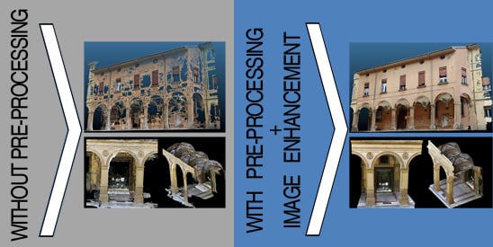
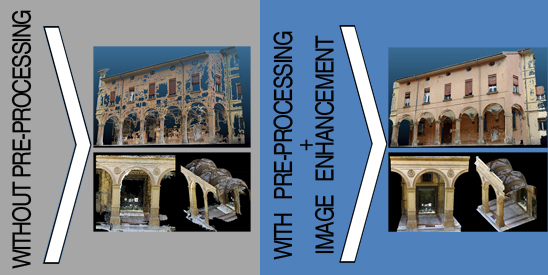
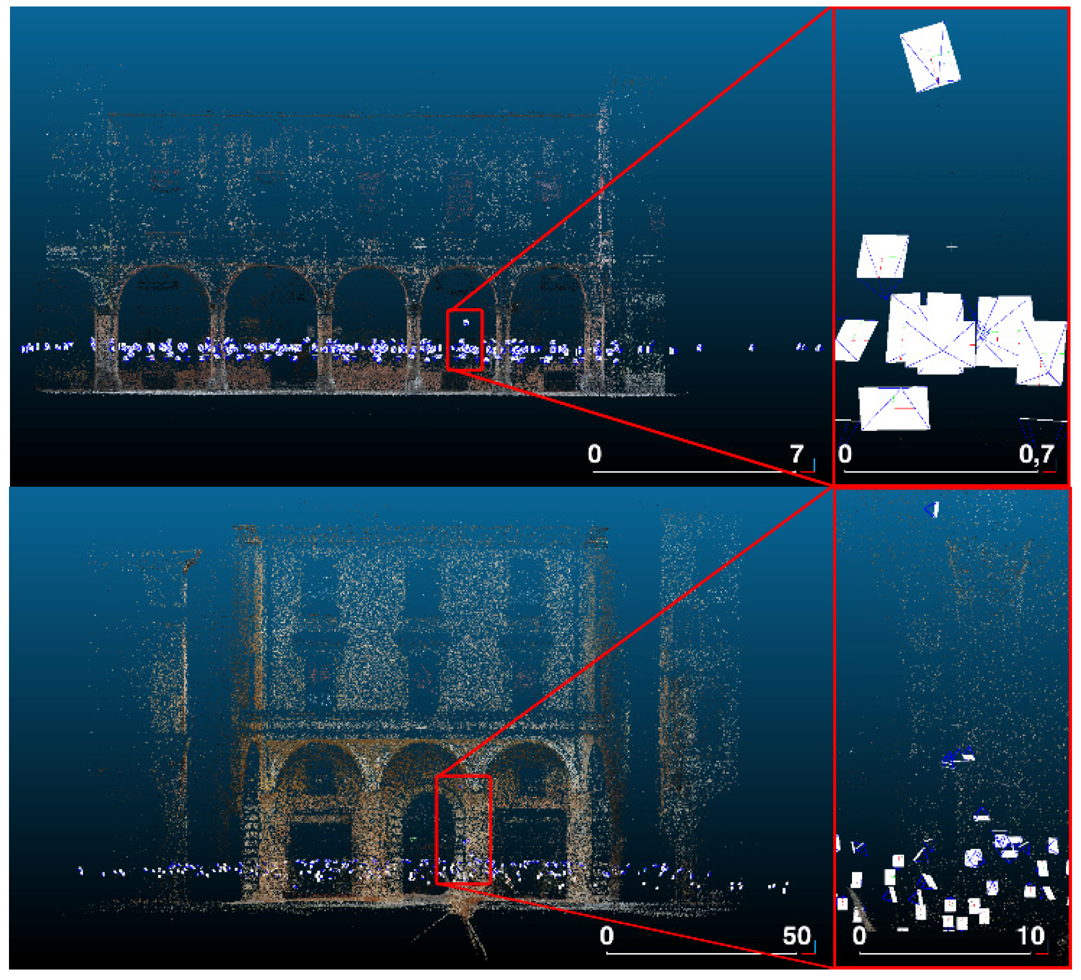
For terrestrial applications, the level of automation is reaching very high standards and it is increasing the impression that few randomly acquired images (or even found on the Internet) and a black-box tool (or mobile app) are sufficient to produce a metrically precise 3D point cloud or textured 3D model. Such tools are able to ingest and process large quantities of images almost always delivering an apparently successful solution, which is often a local minimum and not the fully correct one (
Figure 2). However, non-expert users might not be able to spot such small errors or divergences in the bundle adjustment due to the fact that only a message of successful image orientation is provided, without statistical analyses.
Motion blur, sensor noise and jpeg artifacts are just some of the possible image problems that are negatively affecting automated 3D reconstruction methods. These problems are then coupled with lack of texture scenarios, repeated patterns, illumination changes, etc. Therefore, image pre-processing methods are fundamental to improve the image quality for successful photogrammetric processing. Indeed, as the image processing is fully automated, the quality of the input images, in terms of radiometric quality as well as network geometry, is fundamental for a successful 3D reconstruction.
This paper presents an efficient image pre-processing methodology developed to increase the processing performances of the two central steps of the photogrammetric pipeline,
i.e., image orientation and dense image matching. The main idea is to minimize typical failure caused by Scale-Invariant Feature Transform (SIFT)-like algorithms [
7] due to changes in the illumination conditions or low contrast blobs areas and to improve the performances of dense image matching methods [
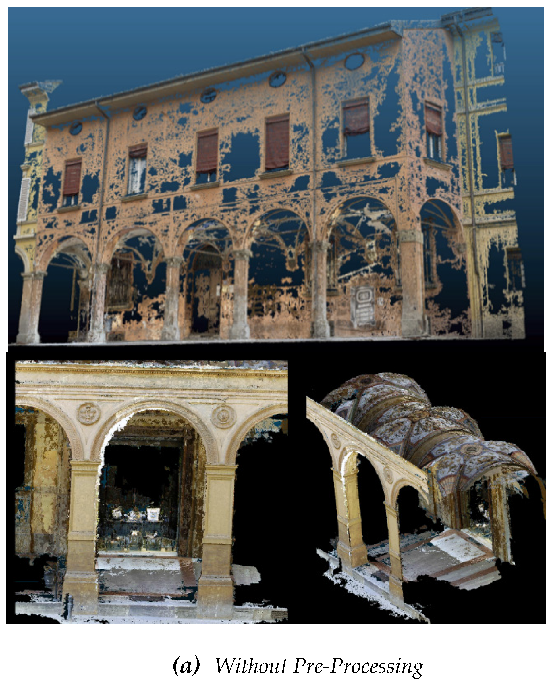
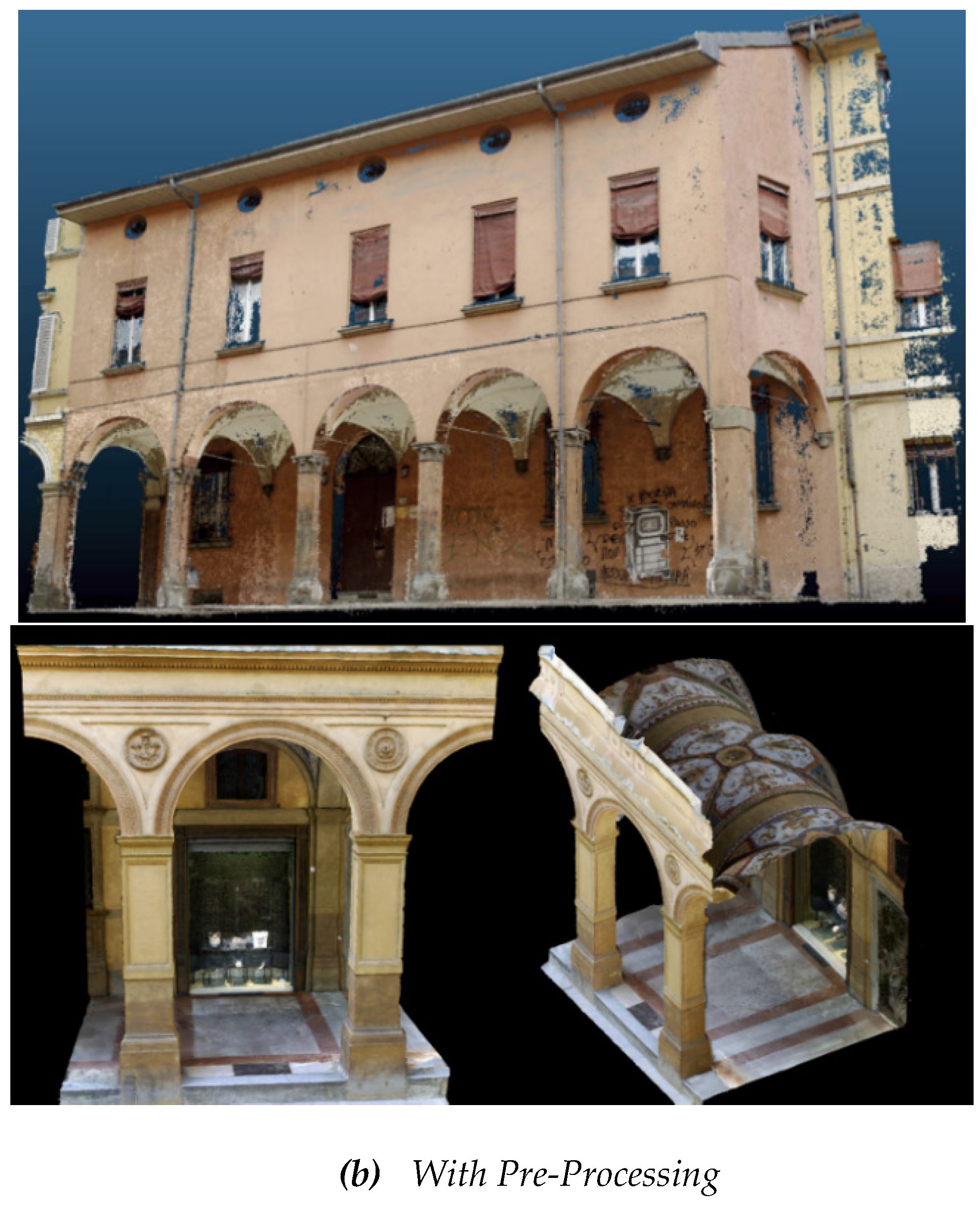
8]. The methodology tries to: (i) increase the number of correct image correspondences, particularly in textureless areas; (ii) track image features along the largest number of images to increase the reliability of the computed 3D coordinates; (iii) correctly orient the largest number of images; (iv) deliver sub-pixel accuracy at the end of the bundle adjustment procedure; and (v) provide dense, complete and noise-free 3D point clouds (
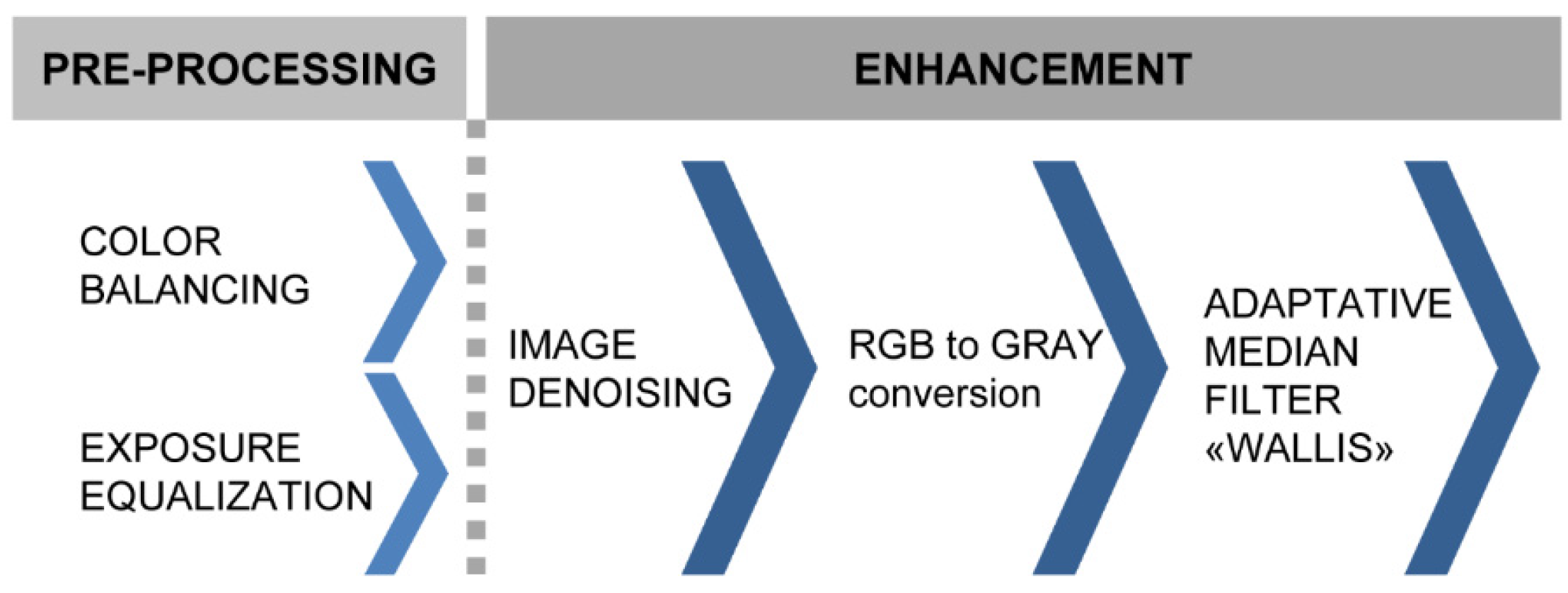
Figure 3). The work investigated various state-of-the-art algorithms aiming to adapt the most promising methods and give solutions at the aforementioned specific problems, thus creating a powerful solution to radiometrically improve the image quality of an image datasets. The developed procedure for image pre-processing and enhancement consists of color balancing (
Section 2), image denoising (
Section 3), color-to-gray conversion (
Section 4) and image content enrichment (
Section 5). The pre-processing methodology could be really useful in the architectural, built heritage and archaeological fields, where automated 3D modeling procedures have become very common whereas skills in image acquisition and data processing are often missing. Our methodology could even be embedded in different types of processing scenarios, like completely automated web-based applications (e.g., Autodesk ReCap and Arc 3D Webservice) or offline desktop-based applications (e.g., Agisoft Photoscan, Photometrix iWitness, VisualSFM, and Pix4D Mapper).
The pipeline (
Figure 4) is afterwards presented and evaluated using some datasets of architectural scenarios.
Related Works
Image pre-processing is a set of methods used to increase the quality of images for successive processing purposes [
9]. The aim is thus to enhance some image features important, e.g., for 3D reconstruction algorithms or to remove unwanted disturbs or degradations in the image. A pre-processing can be a simple histogram’s stretching or a more complex approach like denoising or filtering [
10,
11]. Image pre-processing normally comprises enhancement (
i.e., the improvement of the image quality) and restoration (
i.e., the removal of degraded areas). The former is more subjective, whereas the latter is an objective process that involves the modeling of degradation (possibly from prior knowledge) and applying an inverse process to recover the original signal. Image pre-processing is a fundamental task for many successive tasks in applications like medical imaging [
12], computer vision, underwater photogrammetry [
13] or 3D modeling [
14].
Maini and Aggarwal [
15] provide an overview of concepts and algorithms commonly used for image enhancement. Stamos
et al. [
16] presents some metrics to estimate the amount of blur in image sequence, based on color saturation, local auto-correlation and gradient distribution. Feature tracking and camera poses recovery methods in blurry image sequences can be improved using edgelets [
17] or blurring the previous frame in order to obtain a consistent tracking [
18] or deblurring a current frame with a blur kernel [
19]. Guidi
et al., [
14] analyses how image pre-processing with polarizing filters and HDR imaging may improve indoor automated 3D reconstruction processes based on SfM methods. Verhoeven
et al. [
20] investigated the use of different grayscale conversion algorithms to decolorize color images as input for SfM software packages. Bellavia
et al. [
21] presented an online pre-processing strategy to detect and discard bad frames in video sequences. The method is based on the Double Window Adaptive Frame Selection (DWAFS) algorithm which works on a simple gradient statistic (gradient magnitude distribution). The percentile statistic of each frame is used to develop an adaptive decision strategy based on a dangling sample window according to the time series of the ongoing percentile values and the last best ones.
2. Color Balance and Exposure Equalization
Color balance is the global adjustment of the intensity of the (red, green, and blue) colors in order to render them correctly. Color balance and exposure equalization is a key step to ensure: (i) faithful color appearance of a digitized artifact; and (ii) consistency of the color-to-gray conversion. This latter one (see
Section 4) is a fundamental step as all feature extraction and image matching algorithms works using only the luminance channel. A correct color balance allows minimizing the typical problem of incorrectly detected areas (e.g., different luminance value for the same color and/or isoluminant colors) that strongly appear in case of surfaces of the same color or colors with the same luminance value. Therefore, the color balance procedure aims to produce radiometrically-calibrated images ensuring the consistency of surface colors in all the images (
i.e., as much as possible similar RGB values for homologous pixels). Starting from captured RAW images, our workflow includes (
Section 2.2): exposure compensation, optical correction, sharpen, and color balance.
2.1. Color Spaces
The use of an appropriate color space to work and render images on screen is fundamental.
sRGB, a standard RGB color space created cooperatively by HP and Microsoft in 1996, is certainly the best choice as output color space for textures and to display rendered 3D models for several reasons including:
sRGB is the default color space for HTML, CSS, SMIL and other web standards;
sRGB is consistent among different monitors or video-projectors; and
sRGB is implemented in the OpenGL graphic libraries, used in many rendering software.
However, the sRGB color space is very narrow and may produce loss of information, mainly in the acquisition and processing phases. To avoid these problems, a broader rendered color space is used, such as the Adobe-RGB (1998), which represents an excellent compromise between the amount of colors that can be codified and the possibility of displaying them on the screen. The use of Adobe-RGB (1998) allows avoiding possible inaccuracies of the sRGB color space in shadows (~25% luminance) as well as highlights (~75% luminance). Adobe-RGB (1998) expands its advantages to areas of intense orange, yellow and magenta color. As the sRGB is a “de facto” standard for consumer cameras storing images in JPEG format, it is advisable to use the RAW format, which normally map to a rendered color space as the Adobe-RGB or sRGB color space.
2.2. Proposed Approach
Between the two general approaches (color characterization
vs. spectral sensitivities based on color targets) [
22] we adopted this last technique that uses a set of differently colored samples measured with a spectrophotometer.
The most precise characterization for any given camera requires recording its output for all possible
stimuli and comparing it with separately measured values for the same
stimuli [
23]. However, storage of such a quantity of data is impractical, and, therefore, the response of the device is captured for only a limited set of
stimuli—normally for the acquisition conditions. The responses to these representative
stimuli can then be used to calibrate the device for input
stimuli that were not measured, finding the transformation between measured CIExyz values and stored RGB values. To find this transformation, several techniques have been developed, including look-up tables [
24].
The method for evaluating and expressing color accuracy (“color characterization”) includes a physical reference chart acquired under standard conditions, a reference chart color space with the ideal data values for the chart, a way to relate or convert the device color space to the reference chart color space and, finally, a way to measure and show errors in the device’s rendering of the reference chart. The target GretagMacbeth ColourChecker [
25] is employed during the image acquisitions, considering the measurements of each patch as reported in Pascale [
26].
A captured color image containing the GretagMacbeth ColourChecker is neutralized, balanced and properly exposed. Using in-house software, an ICC (International Color Consortium) profile—assigned together with the Adobe-RGB (1998) color space of the RAW image—is generated. Before creating ICC profiles, a standard gamma correction (γ = 2.2) is applied, converting all images to the camera’s native linear color space, thus improving the quality of the profiles. A protocol is developed to use the same calibration for groups of images with the same features (i.e., orientation, exposure and framed surfaces) thus to maintain consistency in the process and results.
The color accuracy is computed in terms of the mean camera chroma relative to the mean ideal chroma in the CIE color metric (
ΔE*00) as defined in 2000 by CIE [
27]:
This formula is a new version of the original one (1976) and is more suitable for our uses. It takes into consideration the problem of non-perceptual uniformity of the colors for which
ΔE*00 varies the weight of
L* depending on where the brightness range falls. Song and Luo [
28] showed that the perceptible and acceptable color differences in complex images presented on a CRT (Cathode Ray Tube) monitor are approximately 2.2 and 4.5, respectively. In our case, the latter value was used as a strict reference for accuracy, defined from perception tests on the results obtained using this value.
Exposure error in f-stops was also evaluated on the plane of the target assumed as one the main object captured in the image. The ΔE*00 and the exposure error calculations was computed using Imatest Studio software version 3.9.
From an operational point of view, the preservation of color fidelity throughout the image processing is ensured by:
taking pictures in the most homogeneous operative conditions (aperture/exposure direction and intensity of light);
including ColourChecker target inside the photographed scenes in order to correct the image radiometry;
storing photos in RAW format; and
using an appropriate color space from the beginning of the image processing.
An important and critical issue is the acquisition of the color target. In order to maintain uniform lighting in an external environment, for each image, we need to consider: (i) surfaces illuminated and oriented as the ColourChecker and that presents an angle of incidence with sunlight of approximately 20°–45° or (ii) image acquisitions performed with overcast sky. To minimize the light glare, that would give unexpected results in the calibration process, the ColourChecker is normally placed on a tripod with a dark background and orthogonal to the camera optical axis. Finally, we verified that a ColourChecker image width of 500 to 1500 pixels is sufficient for ΔE*00 analysis, as also suggested in the Imatest user guide.
3. Image Denoising
Image noise is defined in the ISO 15739 standard as “unwanted variations in the response of an imaging system” [
29]. It is formed when incoming light is converted from photons to an electrical signal and originates from the camera sensor, its sensitivity and the exposure time as well as by digital processing (or all these factors together). Noise can appear in different ways:
Fixed pattern noise (“hot” and “cold” pixels): It is due to sensor defects or long time exposure, especially with high temperatures. Fixed pattern noise always appears in the same position.
Random noise: It includes intensity and color fluctuations above and below the actual image intensity. They are always random at any exposure and more influenced by ISO speed.
Banding noise: It is caused by unstable voltage power and is characterized by the straight band in frequency on the image. It is highly camera-dependent and more visible at high ISO speed and in dark image. Brightening the image or white balancing can increase the problem.
Luminance noise (i.e., a variation in brightness): It is composed of noisy bright pixels that give the image a grainy appearance. High-frequency noise is prevalent in the luminance channel, which can range from fine grain to more distinct speckle noise. This type of noise does not significantly affect the image quality and can be left untreated or only minimally treated if needed.
Chrominance noise (i.e., a variation in hue): It appears as clusters of colored pixels, usually green and magenta. It occurs when the luminance is low due to the inability of the sensor to differentiate color in low light levels. As a result, errors in the way color is recorded are visible and hence the appearance of color artifacts in the de-mosaicked image.
Starting from these considerations, the noise model can be approximated with two components:
- (a)
A signal-independent Gaussian noise to compensate for the fixed pattern noise (FPN).
- (b)
A signal-dependent Poisson noise to compensate for the temporal (random) noise, called Shot Noise.
A denoise processing basically attempts to eliminate—or at least minimize—these two components.
Several denoising methods [
30,
31,
32] deal directly with Poisson noise. Wavelet-based denoising methods [
33,
34] adapt the transform threshold to the local noise level of the Poisson process. Recent papers on the Anscombe transform by Makitalo and Foi [
35] and Foi [
36], argue that, when combined with suitable forward and inverse variance-stabilizing transformations (VST), algorithms designed for homoscedastic Gaussian noise work just as well as
ad-hoc algorithms based on signal-dependent noise models. This explains why the noise is assumed to be uniform, white and Gaussian, having previously applied a VST to the noisy image to take into account the Poisson component.
An effective restoration of image signals will require methods that either model the signal a-priori (
i.e., Bayesian) or learn the underlying characteristics of the signal from the given data (
i.e., learning, non-parametric, or empirical Bayes’ methods). Most recently, the latter approach has become very popular, mainly using patch-based methods that exploit both local and non-local redundancies and “self-similarities” in the images [
24]. A patch-based algorithm denoises each pixel by using knowledge of (a) the patch surrounding it and (b) the probability density of all existing patches.
Typical noise reduction software reduces the visibility of noise by smoothing the image, while preserving its details. The classic methods estimate white homoscedastic noise only, but they can be adapted easily to estimate signal- and scale-dependent noise.
The main goals of image denoising algorithms are:
perceptually flat regions should be as smooth as possible and noise should be completely removed from these regions;
image boundaries should be well preserved and not blurred;
texture detail should not be lost;
the global contrast should be preserved (i.e., the low-frequencies of denoised and input images should be equal); and
no artifacts should appear in the denoised image.
All these goals are appropriate also for our cases were we need not to remove signal, nor distort blob shape and intensity areas to have efficient keypoint extraction and image matching processing.
Numerous methods were developed to meet these goals, but they all rely on the same basic method to eliminate noise: averaging. The concept of averaging is simple, but determining which pixels to average is not.
In summary:
the noise model is different for each image;
the noise is signal-dependent;
the noise is scale-dependent; and
the knowledge of each dependence is crucial to proper denoising of any given image which is not raw, and for which the camera model is available.
To meet this challenge, four denoising principles are normally considered:
transform thresholding (sparsity of patches in a fixed basis);
sparse coding (sparsity on a learned dictionary);
pixel averaging and block averaging (image self-similarity); and
Bayesian patch-based methods (Gaussian patch model).
Each principle implies a model for the ideal noiseless image. The current state-of-the-art denoising recipes are in fact a smart combination of all these ingredients.
3.1. Evaluated Methods
We investigated different denoise algorithms, some commercial, namely:
Imagenomic Noiseware [
37,
38]: It uses hierarchical noise reduction algorithms, subdividing the image noise into two categories: luminance noise and color noise, furthermore divided into frequencies ranging from very low to high. The method includes detection of edges and processing at different spatial frequencies, using the YCbCr color space. Noiseware presents good quality results and it is easy to set-up.
Adobe Camera RAW denoise [
39]: Noise-reduction available in Camera Raw 6 with Process 2010 (in
Section 6 simply called
Adobe) uses a luminance noise-reduction technique based on a wavelet algorithm that seeks to determine extremely high-frequency noise and to separate it from high-frequency image texture. The method is capable of denoising large noisy areas of an image as well as to find and fix “outliers”,
i.e., localized noisy areas. Unfortunately, the method is a global filter and it needs a skilled manual intervention for each image to set-up the right parameters.
Non-Local Bayesian filter [
40,
41,
42]: It is an improved patch-based variant of the Non Local-means (NL-means) algorithm, a relatively simple generalization of the Bilateral Filter. In the NL-Bayes algorithm, each patch is replaced by a weighted mean of the most similar patches present in a neighborhood. To each patch is associated a mean (which would be the result of NL-means), but also a covariance matrix estimating the variability of the patch group. This allows computing an optimal (Bayesian minimal mean square error) estimate of each noisy patch in the group, by a simple matrix inversion. The implementation proceeds in two identical iterations, but the second iteration uses the denoised image of the first iteration to estimate better the mean and covariance of the patch models.
Noise Clinic [
43,
44,
45,
46]: It is the conjunction of a noise estimation method and of a denoising method. Noise estimation is with an extension of [
47] method to be able to estimate signal-dependent noise, followed by multiscale NL-Bayes denoising method. The multiscale denoising follow these principles: (a) signal dependent noise estimated at each scale; and (b) zoom down followed by Anscombe transform to whiten the noise at each scale; denoising performed at each scale, bottom-up (coarse to fine). Noise Clinic is implemented in DxO Optics Pro with the name of Prime (Probabilistic Raw IMage Enhancement), and it is useful for very noisy and high-ISO RAW images, or for photos taken with an old camera that could not shoot good-quality images at ISO higher than 1600 ISO.
Color Block Matching 3D (
CBM3D) filter [
48]: A color variant of Block Matching 3D (BM3D) filter [
49]. BM3D is a sliding-window denoising method extending the Discrete Cosine Transform (DCT) [
25] and NL-means algorithms. BM3D, instead of adapting locally a basis or choosing from a large dictionary, uses a fixed basis. The main difference from DCT denoising is that a set of similar patches is used to form a 3D block, which is filtered by using a 3D transform, hence the name “collaborative filtering”. The algorithm works in two stages: “basic estimate” of the image and the creation of the final image, and with four steps each stage: (a) finding the image patches similar to a given image patch and grouping them in a three-dimensional block: (b) 3D linear transform of the 3D block; (c) shrinkage of the transform spectrum coefficients; and (d) inverse three-dimensional transformation. This second step mimics the first step, with two differences. The first difference is that it compares the filtered patches instead of the original patches. The second difference is that the new 3D group is processed by an oracle Wiener filter, using coefficients from the denoised image obtained at the first step to approximate the true coefficients. The final aggregation step is identical to that of the first step. CBM3D extends the multi-stage approach of BM3D via the YoUoVo color system. CBM3D produces a basic estimate of the image, using the luminance data, and delivers the denoised image performing a second stage on each of the three color channels separately. This generalization of the BM3D is non-trivial because authors do not apply the grayscale BM3D independently on the three luminance-chrominance channels but they impose a grouping constraint on both chrominance. The grouping constraint means that the grouping is done only once, in the luminance (which typically has a higher SNR than the chrominance), and exactly the same grouping is reused for filtering both chrominance. The constraint on the chrominance increases the stability of the grouping with respect to noise. With this solution, the quality of denoised images is also excellent for moderate noise levels.
3.2. Proposed Approach
Following the experiment results, an in-house method (named
CBM3D-new) was developed starting from the CBM3D approach [
48]. For every image of a dataset, the method automatically select the necessary parameters based on the type of camera, ISO sensitivity and stored color profiles. In particular, the processing selection of the latter one is based on image features and camera capabilities: dealing with professional or prosumer setups, when source images are stored as RAW images or in non-RAW formats characterized by a wide color space such as the Adobe-RGB (1998), then opponent color space are chosen. When source images are stored in JPG format using a relatively narrower color space, such as sRGB—the most used in consumer cameras—then YCbCr color space is chosen.
The camera ISO is strictly related to the image noise. The sigma parameter, i.e., the standard deviation of the noise, increases when the ISO increases, ranging from lower values (σ = 1 for images shot at less than 100 ISO) to higher ones (σ = 10 for images shot at more than 800 ISO). ISO sensitivity similarly influences other filtering parameters, such as the number of sliding step to process every image block (ranging from 3 to 6), the length of the side of the search neighborhood for full-search block-matching (ranging from 25 to 39) as well as the number of step forcing to switch to neighborhood full-search (ranging from 1 to 36).
4. Color-to-Gray
Most of the algorithms involved in the image-based 3D reconstruction pipeline (mainly feature extraction for tie points identification and dense image matching) are conceptually designed to work on grayscale images (
i.e., single-band images) instead of the RGB triple. This is basically done to highly reduce the computational complexity of the algorithms compared to the utilization of the three channels. Color to grayscale conversion (or decolorization) can be seen as a dimensionality reduction problem and it should not be underestimated, as there are many different properties that need to be preserved. Over the past decades, different color-to-gray algorithms have been developed to derive the best possible decolorized version of a color image [
20]. All of them focus on the reproduction of color images with grayscale mediums, with the goal of: (i) a perceptual accuracy in terms of the fidelity of the converted image; and (ii) a preservation of the color contrast and image structure contained in the original color also in the final decolorized image. Nevertheless, these kinds of approaches are not designed to fulfill the needs of image matching algorithms where local contrast preservation is crucial during the matching process. This was also observed in Lowe [
50] where the candidate key points with low contrast are rejected in order to decrease the ambiguity of the matching process.
Color-to-gray conversion methods can be classified according to their working space:
4.1. Evaluated Methods
We investigated different color-to-gray methods, namely:
GREEN2GRAY: It is a trivial method working in Image Space where the green channel is extracted from a RGB image and used to create the final grayscale image.
Matlab RGB2GRAY: It is a direct method implemented in Matlab and based on the above mentioned weighted sum of the three separate channels.
Decolorize [
55]: The technique performs a global grayscale conversion by expressing the grayscale as a continuous, image-dependent, piecewise linear mapping of the primary RGB colors and their saturation. Their algorithm works in the YPQ color opponent space and aims to perform a contrast enhancement too. The color differences in this color space are projected onto the two predominant chromatic contrast axes and are then added to the luminance image. Unlike a principal component analysis, which optimizes the variability of observations, a predominant component analysis optimizes the differences between observations. The predominant chromatic axis aims to capture, with a single chromatic coordinate, the color contrast information that is lost in the luminance channel. The luminance channel Y is obtained with the NTSC CCIR 601 luma weights. The method is very sensitive to the issue of gamma compression with some risks of decrease of the quality of the results mainly in light areas or dark areas where many features will be lost because the saturation balancing interacts incorrectly with the outlier detection.
Realtime [
56,
57,
58]: This method is based on the consideration that in the human visual system the relationship to the adjacent context plays a vital role to order the different colors. Therefore, the method relaxes the color order constraint and seeks better preservation of color contrast and significant enhancement of visual distinctiveness for edges. For color pairs without a clear order in brightness, a bimodal distribution (
i.e., a mixture of two Gaussians) is performed to automatically find suitable orders with respect to the visual context in optimization. This strategy enables automatically finding suitable grayscales and preserves significant color changes. Practically the method uses a global mapping scheme where all color pixels in the input are converted to grayscale using the same mapping function (a finite multivariate polynomial function). Therefore, two pixels with the same color will have the same grayscale. The technique is today implemented in OpenCV 3.0. In order to achieve real-time performance, a discrete searching optimization can be used.
Adobe Photoshop.
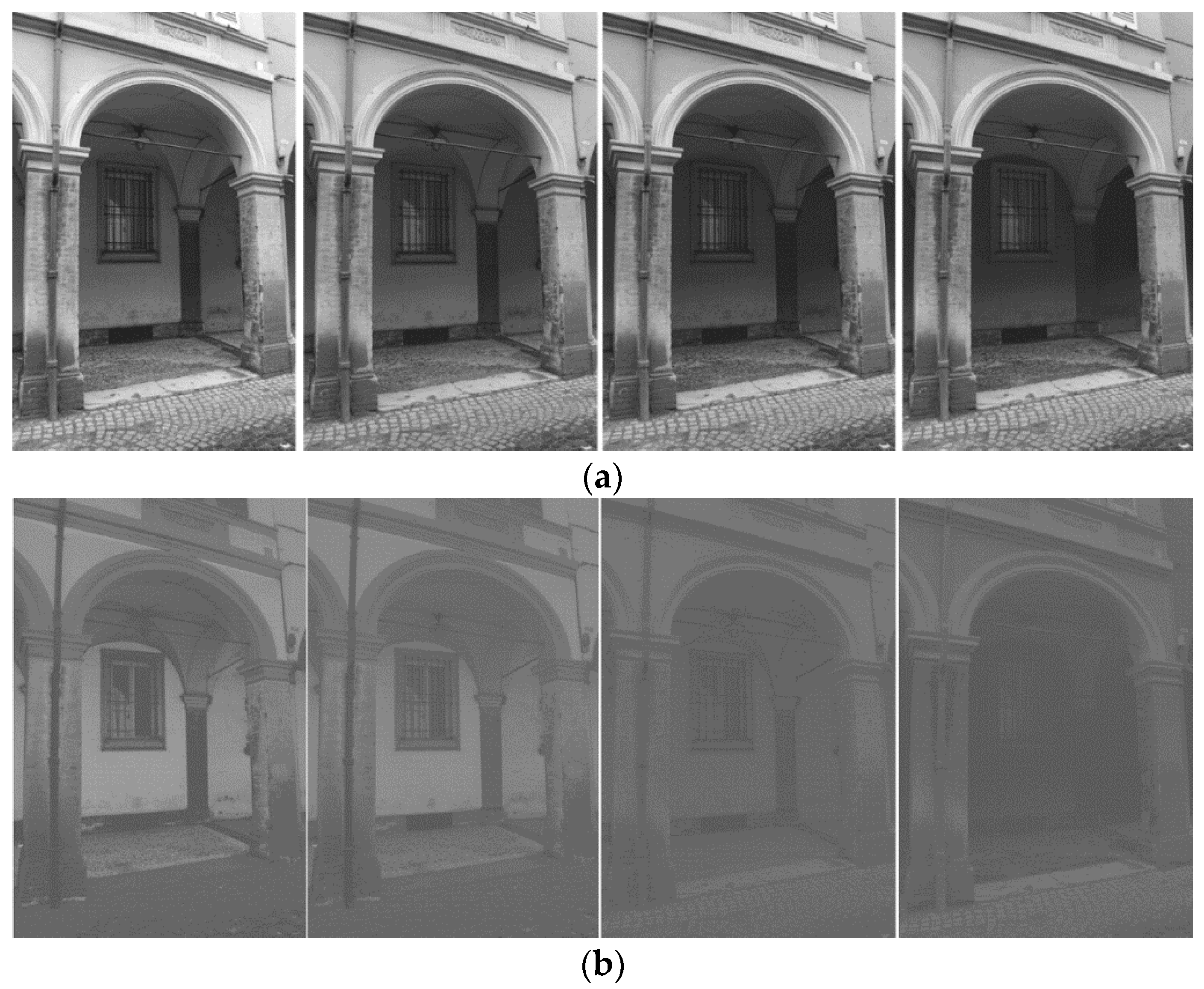
To evaluate the performances of the aforementioned methods (
Figure 5), we applied the pixel-by-pixel difference method applying an offset of 127 levels of brightness to better identify the differences. This technique is the most appropriate to evaluate a method’s efficiency for machine readable process. The simple image subtraction can rapidly provide visual results rather than using CIELAB ΔE*ab or other perceptually-based image comparison methods.
4.2. Proposed Approach
Based on the results achieved with the aforementioned methods, a new decolorization technique, named Bruteforce Isoluminants Decrease (
BID), was developed. The aim of BID is to preserve the consistency between different images considering the following requirements.
Feature discriminability: The decolorization method should preserve the image features discriminability in order to match them in as many images as possible.
Chrominance awareness: The method should distinguish between isoluminant colors.
Global mapping: While the algorithm can use spatial information to determine the mapping, the same color should be mapped to the same grayscale value for every pixel in the image.
Color consistency: The same color should be mapped to the same grayscale value in every image of the dataset.
Grayscale preservation: If a pixel in the color image is already achromatic, it should maintain the same gray level in the grayscale image.
Unsupervised algorithm: It should not need user tuning to work properly, in particular for large datasets.
BID computes the statistical properties of the input dataset with the help of a representative collection of image patches. Differently from the
Multi-Image Decolourize method [
51],
BID is a generalization of the
Matlab RGB2GRAY algorithm, which simultaneously takes in input and analyses the whole set of images that need to be decolorized.
BID has its foundation in the statistics of extreme-value distributions of the considered images and presents a more flexible strategy, adapting dynamically channel weights depending on specific input images, in order to find the most appropriate weights for a given color image.
BID preserves as much as possible the amount of the conveyed information. The algorithm behind
BID tries to maximize the number of peaks obtained in the converted image and to distribute as evenly as possible the amount of tones by evaluating the goodness of a fitting distribution. To calculate the best rectangular fitting, we assumed a 0 slope regression line. The general equation of the regression line is:
where β is equivalent to the average of the histogram points. After calculating the average, the minimum error within all the calculated combinations of channel mixings if sought. The error is calculated as a least squares error:
where
yi are the actual points, while
β is the best linear fitting of the histogram.
BID cyclically varies the amount of red, green and blue and for each variation calculates the distribution of the resulting grayscale image and assesses the fitting quality with respect to a rectangular distribution. Then,
BID chooses the mixing that maximizes the number of tones obtained in the converted image. Finally, similarly to Song
et al. [
59],
BID uses a measurement criterion to evaluate the decolorization quality,
i.e., the newly defined dominant color hypothesis.
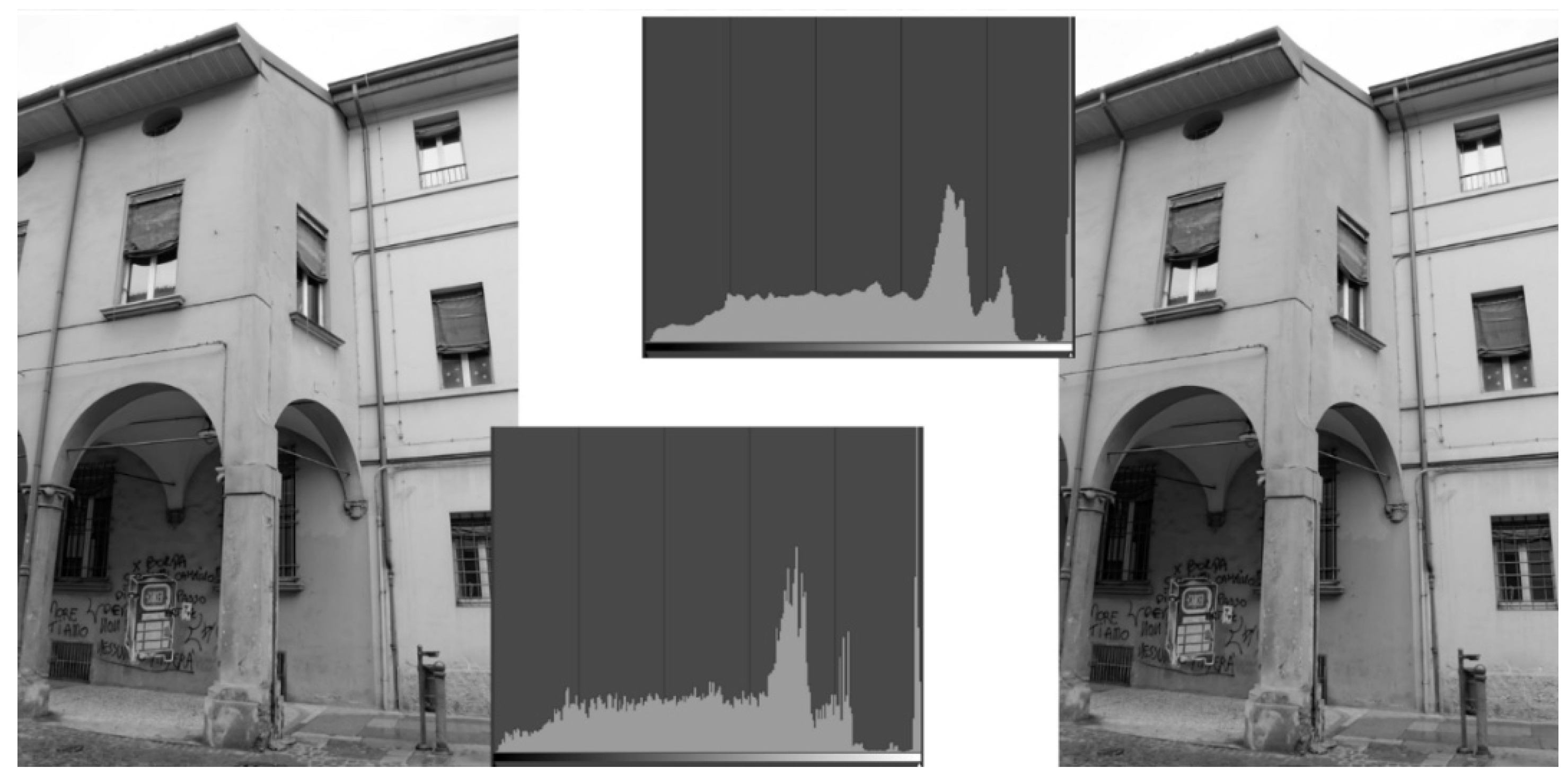
Figure 6 reports an example of
BID results with respect to
Matlab RGB2GRAY method. The main disadvantage of the developed method is the high computational pre-processing time due to the sampled patches on each image of the dataset.
5. Image Content Enhancement with Wallis Filtering
Image contents play a fundamental role in many processing and feature extraction methods. There are various enhancement algorithms to sharp and increase the image quality [
9,
60,
61,
62]. For image-based 3D reconstruction purposes, low-texture surface (such as plaster building facades) causes difficulties to feature detection methods (such as the Difference-of-Gaussian (DoG) function) and matching algorithms, leading to outliers and unsuccessful matching results. Among the proposed methods to enhance image contents, the Wallis filter [
11] showed very successful performances in the photogrammetric community [
63,
64,
65,
66,
67]. Jazayeri
et al. [
68] tested the Wallis filter for different parameters to evaluate its performances for interest point detection and description. Those results demonstrated that an optimum range of values exists and depending on the requirements of the user, but automatic value selection remains undetermined.
The filter is a digital image processing function that enhances the contrast levels and flattens the different exposure to achieve similar brightness of gray level values. The filter uses two parameters to control the enhancement’s amount, the
contrast expansion factor A and the
brightness forcing factor B. The algorithm is adaptive and adjusts pixel brightness values in local areas only, contrary to a global contrast filter, which applies the same level of contrast throughout an entire image. The resulting enhanced image contains greater detail in both low and high-level contrast regions concurrently, ensuring that good local enhancement is achieved throughout the entire image. The Wallis filter requires the user to accurately set a target mean and standard deviation in order to locally adjust areas and match the user-specified target values. Firstly, the filter divides the input image into neighboring square blocks with a user-defined size (“window size”) in order to calculate local statistics. Then, mean (
M) and standard deviation (
S) of the unfiltered image are calculated for each individual block based on the gray values of the pixels and the resulting value is assigned to the central cell of each block. The mean and standard deviation values of all other cells in the block are calculated from this central cell by bilinear interpolation. In this way, each individual pixel gets its own initial local mean and standard deviation based on surrounding pixel values. The user-defined mean and standard deviation values are then used to adjust the brightness and the contrast of the input cells. The resulting enhanced image is thus a weighted combination of the original and user-defined mean and standard deviation of the image. The implementation of the filter of Wallis, given the aforementioned factor A and B, can be summarized as follows:
let S be the standard deviation for the input image;
let M be the mean for the input image;
for each (x,y) pixel in the image,
calculate local mean m and standard deviation s using a NxN neighborhood; and finally
calculate the enhanced output image as
Characterization of Wallis Parameters
The quality of the Wallis filter procedure relies on two parameters: the
contrast expansion factor A and the
brightness forcing factor B. The main difficulty when using the Wallis filter is the correct selection of these parameters, in particular for large datasets, where a unique value of A or B could lead to unsuitable enhanced images. Although several authors reported parameters for successful projects, the filter is more an “
ad-hoc” recipe than an easily deployable system for an automatic photogrammetric pipelines. To overcome this problem and following the achievement presented in [
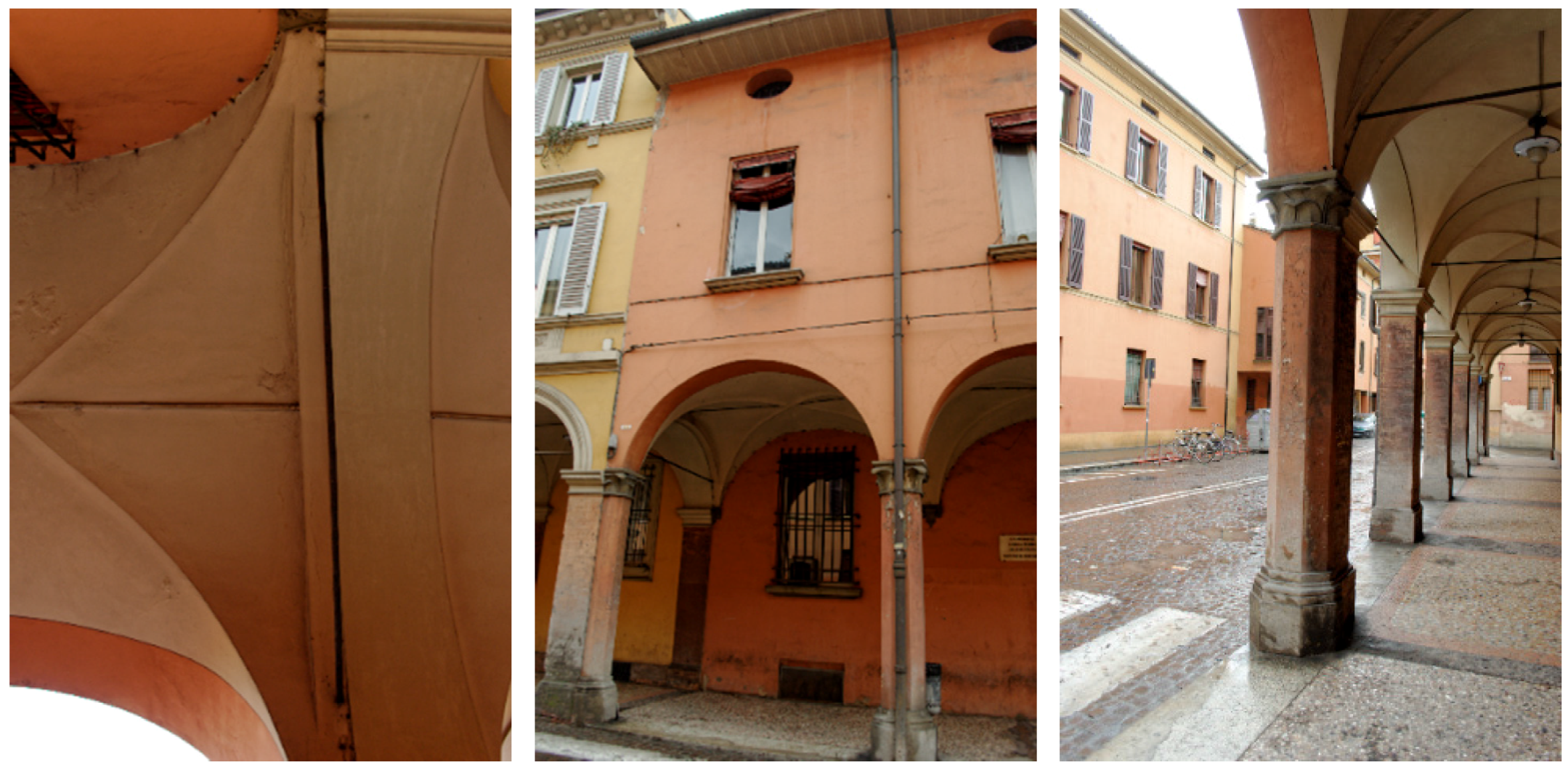
69], a Wallis parameters characterization study was carried out to automatically determine them. Three different datasets, each one composed of three images and involving the majority of possible surveying case studies were used (
Figure 7):
a cross vault characterized by smooth bright-colored plaster;
a building facade and porticoes with smooth plaster; and
a Venetian floor, with asphalt and porphyry cubes with a background facade overexposed and an octagonal pillar in the foreground coated with smooth plaster.
For every dataset, the images were enhanced using different Wallis parameters and then matched to find homologues points using a calibrated version [
7] of the SIFT operator available in Vedaldi’s implementation [
69]. This characterization procedure delivered the following considerations.
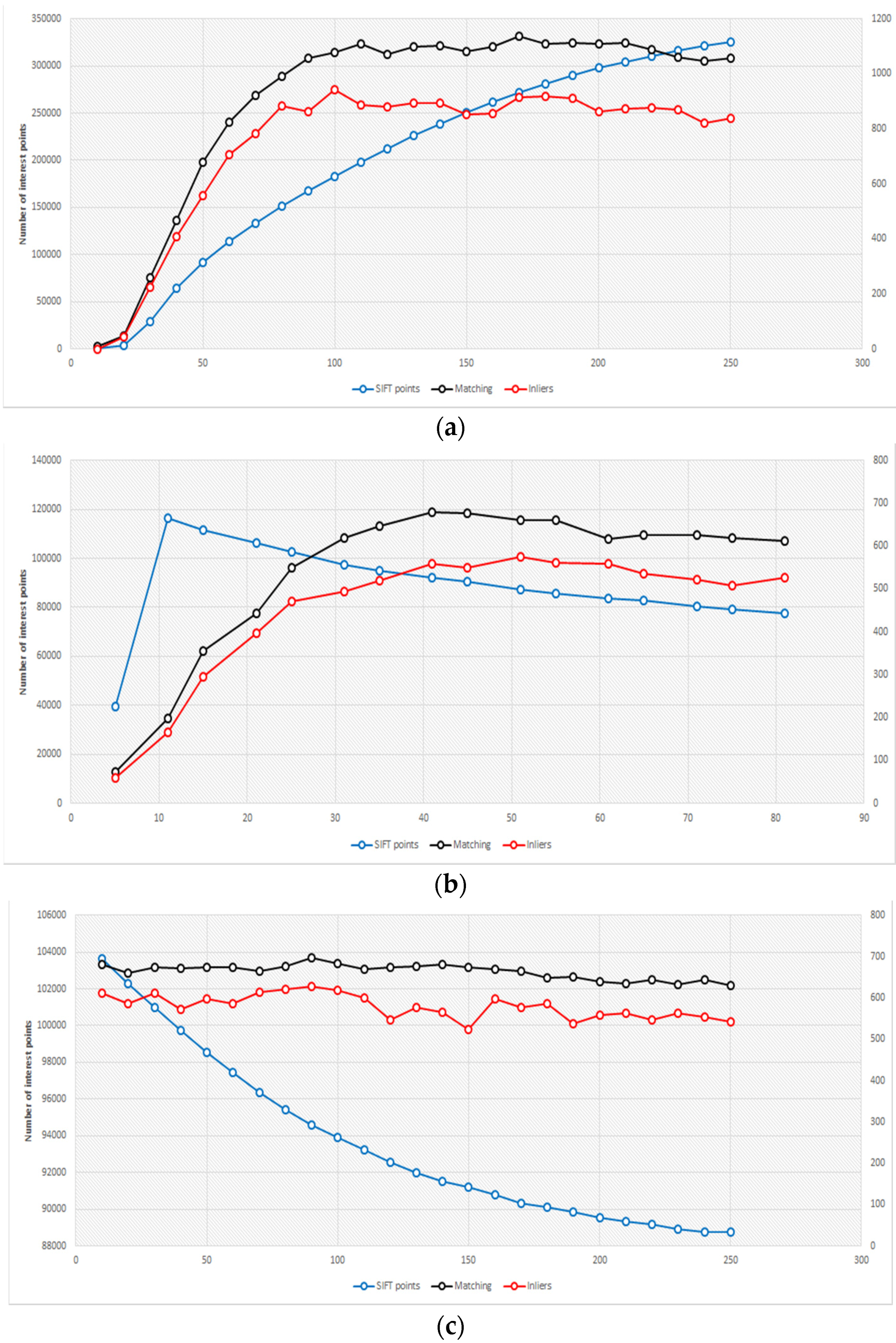
The number of extracted tie points is inversely proportional to the value of the parameter A, but the number of correct matches remains basically stable when varying A, which can then be set at high values to speed up the computation (6–8).
Varying the user-specified standard deviation, the number of tie points and correct matches increases substantially linearly up to a value of 100 and then remains constant (
Figure 8a).
Sensor resolution and window size are linearly related and the increasing of the window size beyond the optimal value does not involve any improvement in either the number of positive matches and in the number of extracted tie points (
Figure 8b).
The mean presents optimal values between 100 and 150 with a decay afterwards (
Figure 8c).
Starting from these observations, a new implementation of the Wallis filter was realized to select the optimal filter parameters and achieve the highest possible ratio of corrected matches with respect to the number of extracted tie points. In particular, the window size parameter is chosen according to the sensor resolution, and presents a linear variation starting from the experimental best values of 41 for a 14 MPixel sensor and 24 for a 10 MPixel sensor. According to our experimental trials, the standard deviation was forcefully set to 60 and the mean to 127. The Contrast Expansion Constant parameter (A) was set to 0.8 to increase the number of detected interest points located in homogeneous and texture-less areas and, alongside, to speed up the computation. The brightness forcing factor (B) according to the experimental results, was set to 1 if the image mean was lower than 150, linearly decreased otherwise, evaluating the entropy of the image.
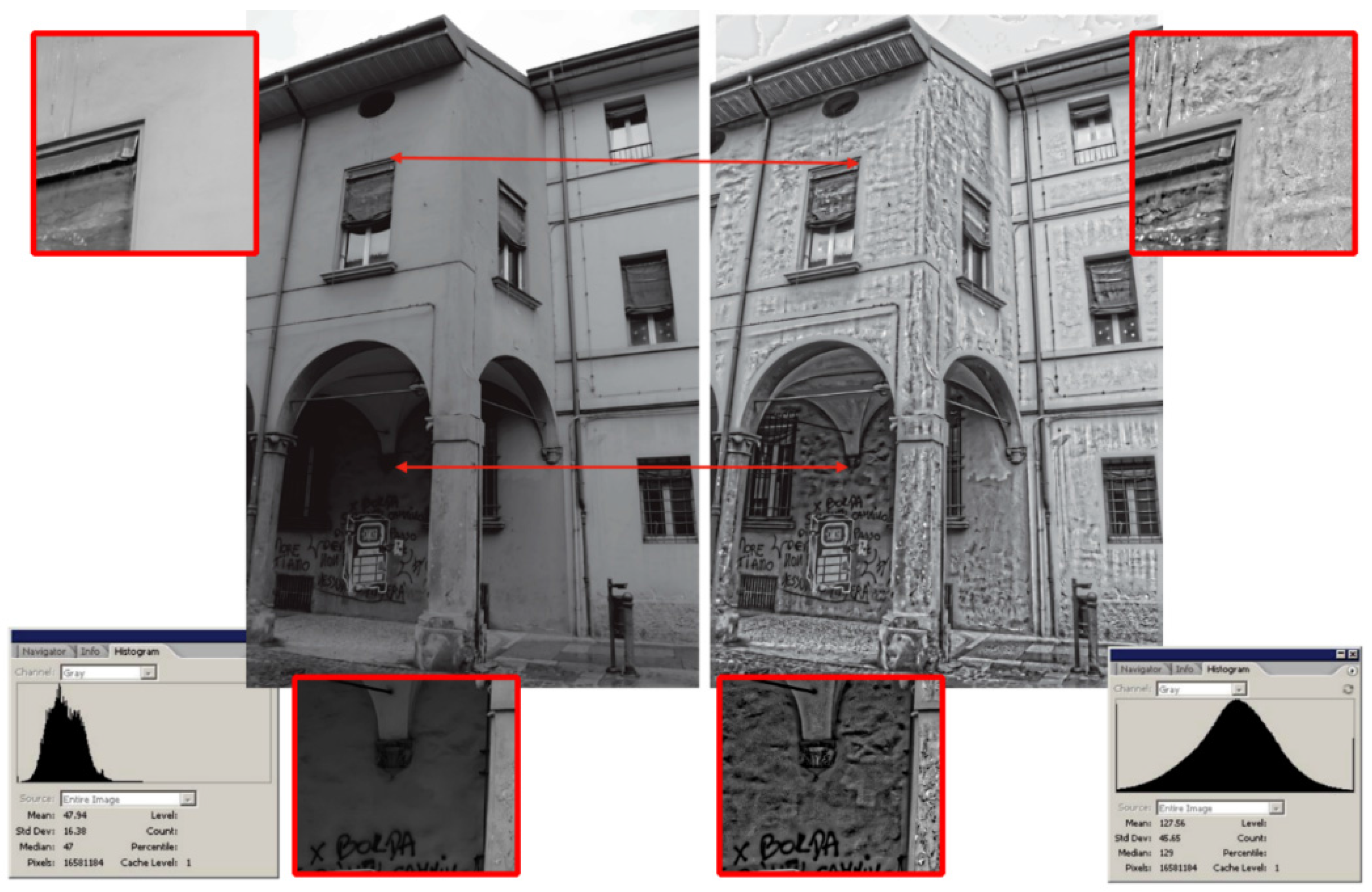
Figure 9 shows the results of Wallis filtering: lower image contents are boosted, whereas a better histogram is achieved.
6. Assessment of the Proposed Methodology
The implemented pre-processing procedure was evaluated on various image networks featuring different imaging configurations, textureless areas and repeated pattern/features. The employed datasets try to verify the efficiency of different techniques in different situations (scale variation, camera rotation, affine transformations, etc.). The datasets contain convergent images, some orthogonal camera rolls and a variety of situations emblematic of failure cases, i.e., 3D scenes (non-coplanar) with homogeneous regions, distinctive edge boundaries (e.g., buildings, windows, doors, cornices, arcades), repeated patterns (recurrent architectural elements, bricks, etc.), textureless surfaces and illumination changes. With respect to other evaluations where synthetic datasets, indoor scenarios, low resolution images, flat objects or simple two-view matching procedures are used and tested, such datasets are more varied with the aim of a complete and precise scene’s 3D reconstruction.
All algorithms are tested and applied to raw images,
i.e., images as close as possible to the direct camera output retaining only the basic in-camera processing: black point subtraction, bad pixel removal, dark frame, bias subtraction and flat-field correction, green channel equilibrium correction, and Bayer interpolation. The datasets are processed with different image orientation software (Visual SFM, Eos Photomodeler and Agisoft Photoscan), trying to keep a uniform number of extracted key points and tie points. Then, dense point clouds are extracted with a unique tool (nFrames SURE). The performances of the pre-processing strategies are reported using:
- (i)
pairwise matching efficiency
i.e., number of correct inlier matches after the RANSAC (RANdom SAmple Consensus) phase normalized with all putative correspondences (
Section 6.1);
- (ii)
- (iii)
- (iv)
an accuracy evaluation of the dense matching results (
Section 6.2).
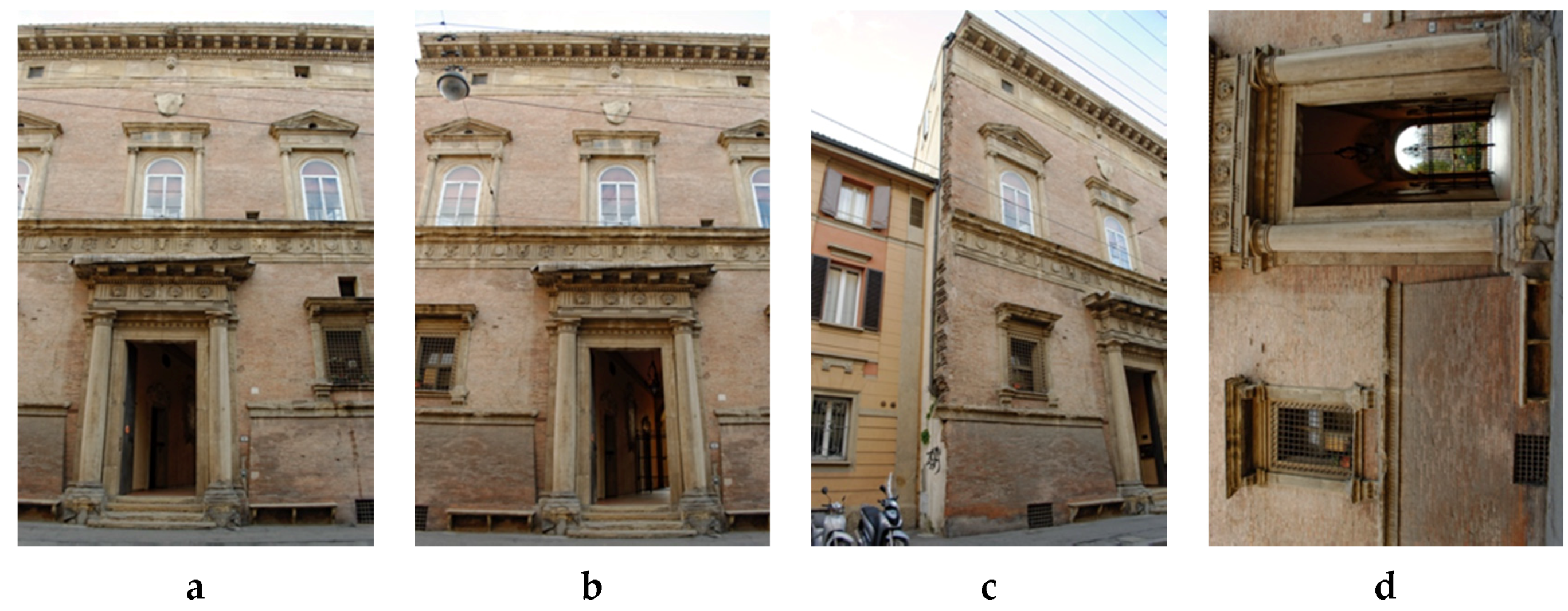
6.1. Dataset 1
The first dataset (four images acquired with a Nikon D3100, sensor size 23.1 × 15.4 mm, 18 mm nominal focal length) shows part of Palazzo Albergati (Bologna, Italy) characterized by repeated brick walls, stone cornices and a flat facade. The camera was moved along the façade of the building, then tilted and rotated (
Figure 10). This set of images is used to evaluate the denoise and color-to-gray techniques with respect to the tie points extraction procedure. The pairwise matching is assessed using three camera movements: (i) parallel with short baseline (a,b); (ii) rotation of
ca. 90° (a–d); and (iii) tilt of
ca. 45° (b,c).
Table 1 reports the computed pairwise matching efficiency after applying the various denoising methods and color-to-gray techniques. The developed methods (
CBM3D-new and
BID) demonstrate a better efficiency in the tie point extraction.
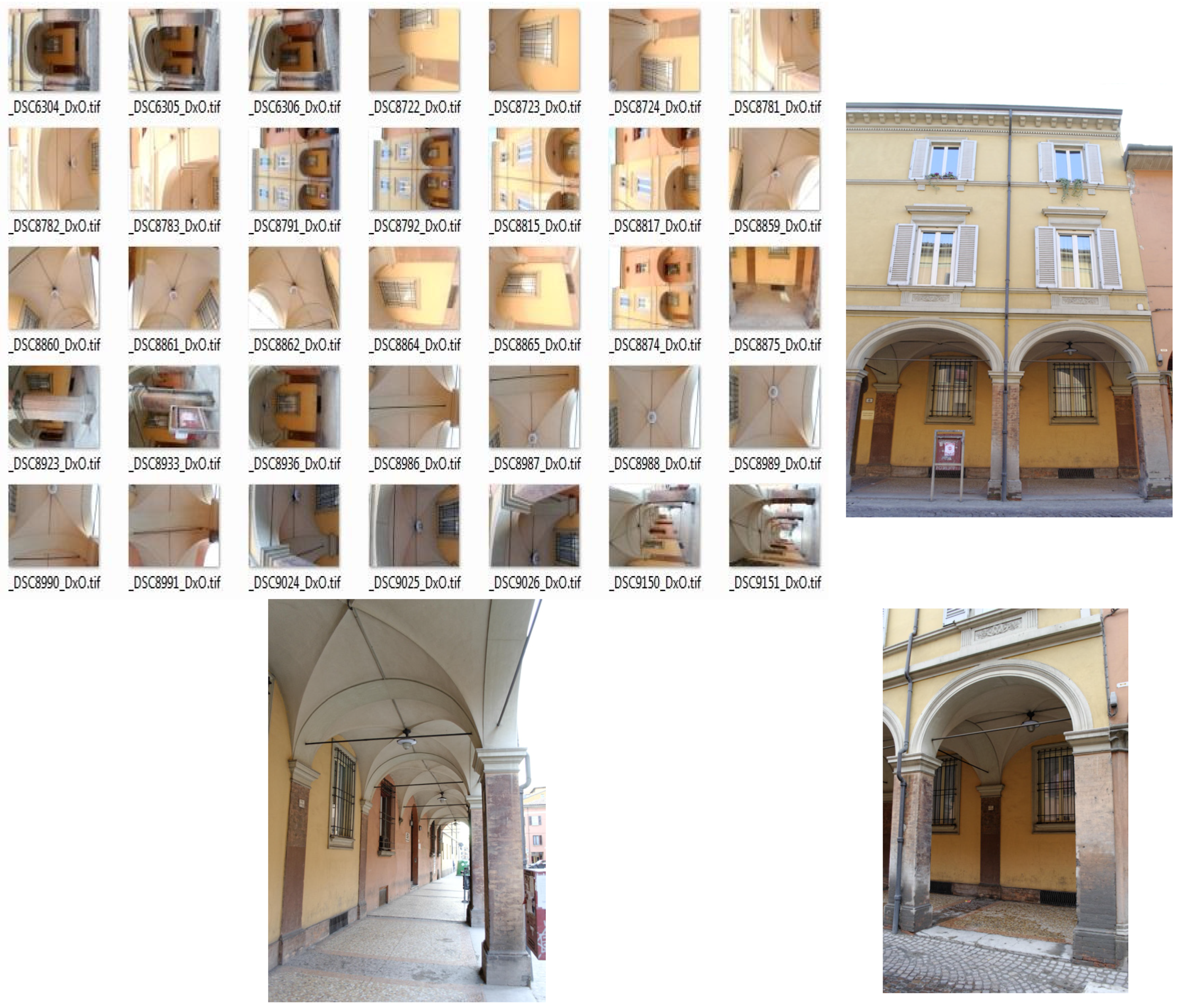
6.2. Dataset 2
The second dataset (35 image acquired with a Nikon D3100, sensor size 23.1 × 15.4 mm, 18 mm nominal focal length) concerns two spans of a three floors building (6 × 11 m) characterized by some arches, pillars, cross vaults and plastered walls with uniform texture. The camera was moved along the porticoes, with some closer shots of the columns (
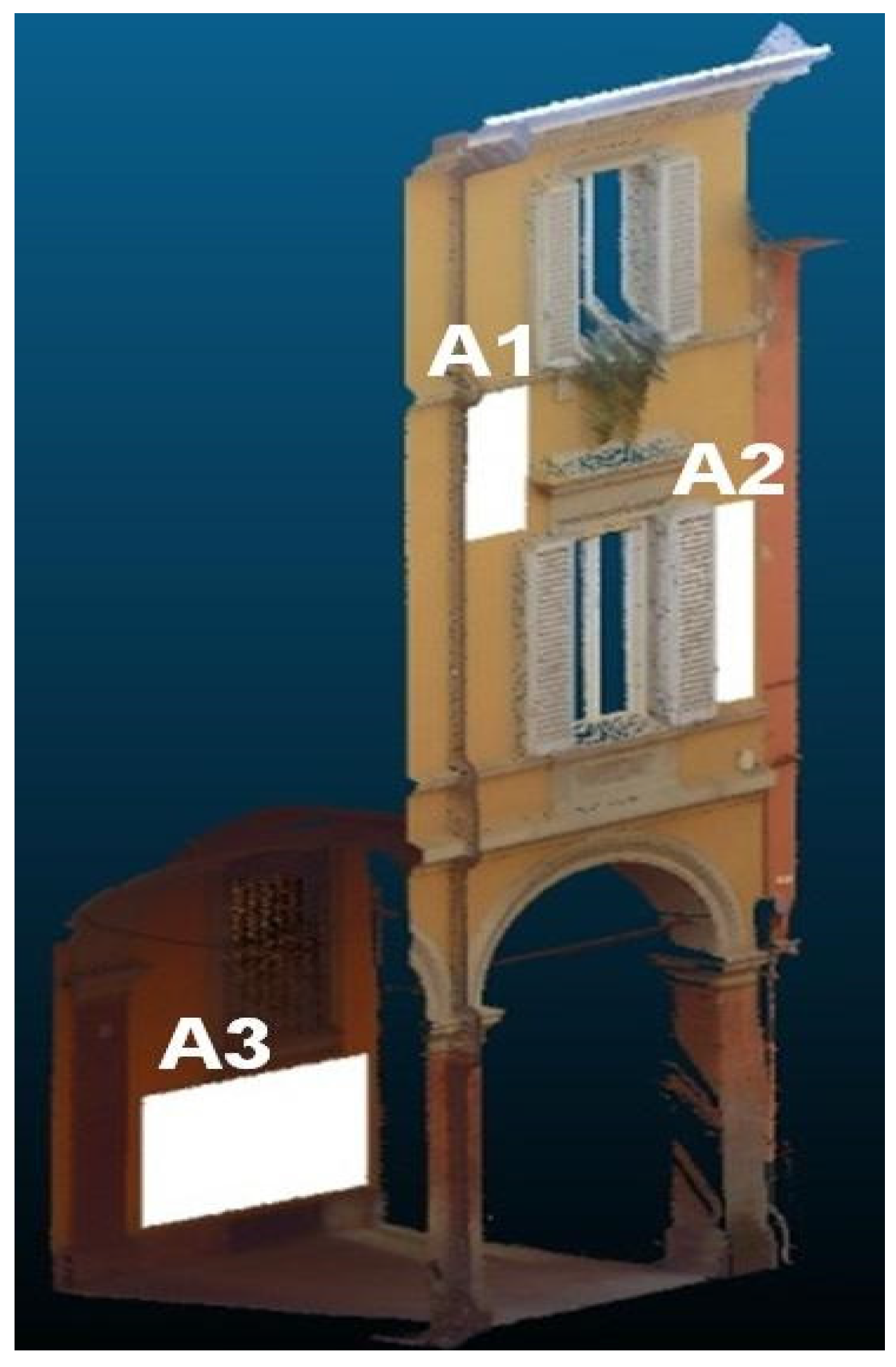
Figure 11). With this dataset we report how color balancing and denoising methodologies help improving the bundle adjustment and dense matching procedures. The accuracy evaluation of the dense matching results is done using a Terrestrial Laser Scanning (TLS) survey as reference (a Faro Focus3D was employed). Three regions (
Figure 12A1–A3) are identified and compared with the photogrammetric dense clouds. The average image GSD (Ground Sample Distance) in the three regions of interest is
ca. 2 mm but the dense matching was carried out using the second-level image pyramid,
i.e., at a quarter of the original image resolution. Therefore, in order to have a reference comparable to the dense matching results, the range data are subsampled to a grid of 5 × 5 mm.
6.2.1. Color Balance Results
The results of the orientation and dense matching steps are reported in
Table 2. The color balancing procedure generally helps in increasing the number of oriented images, except with PS where the dataset is entirely oriented at every run. Furthermore, it helps in deriving denser point clouds.
6.2.2. Image Denoising Results
The denoising methods are coupled to
Matlab RGB2GRAY and Wallis filtering before running the automated orientation and matching procedures. The achieved adjustment results, according to the different denoising methods, show that more images can be oriented (
Table 3) and denser point clouds can be retrieved (
Table 4).
6.2.3. Color-to-Gray Results
The color-to-gray conversion (coupled with the Wallis filtering) shows how algorithms are differently affecting the BA procedure (
Table 5) as well as the dense matching results (
Table 6). It can be generally noticed that the proposed
BID method allows retrieving a larger number of oriented images, a better re-projection errors and denser point clouds.
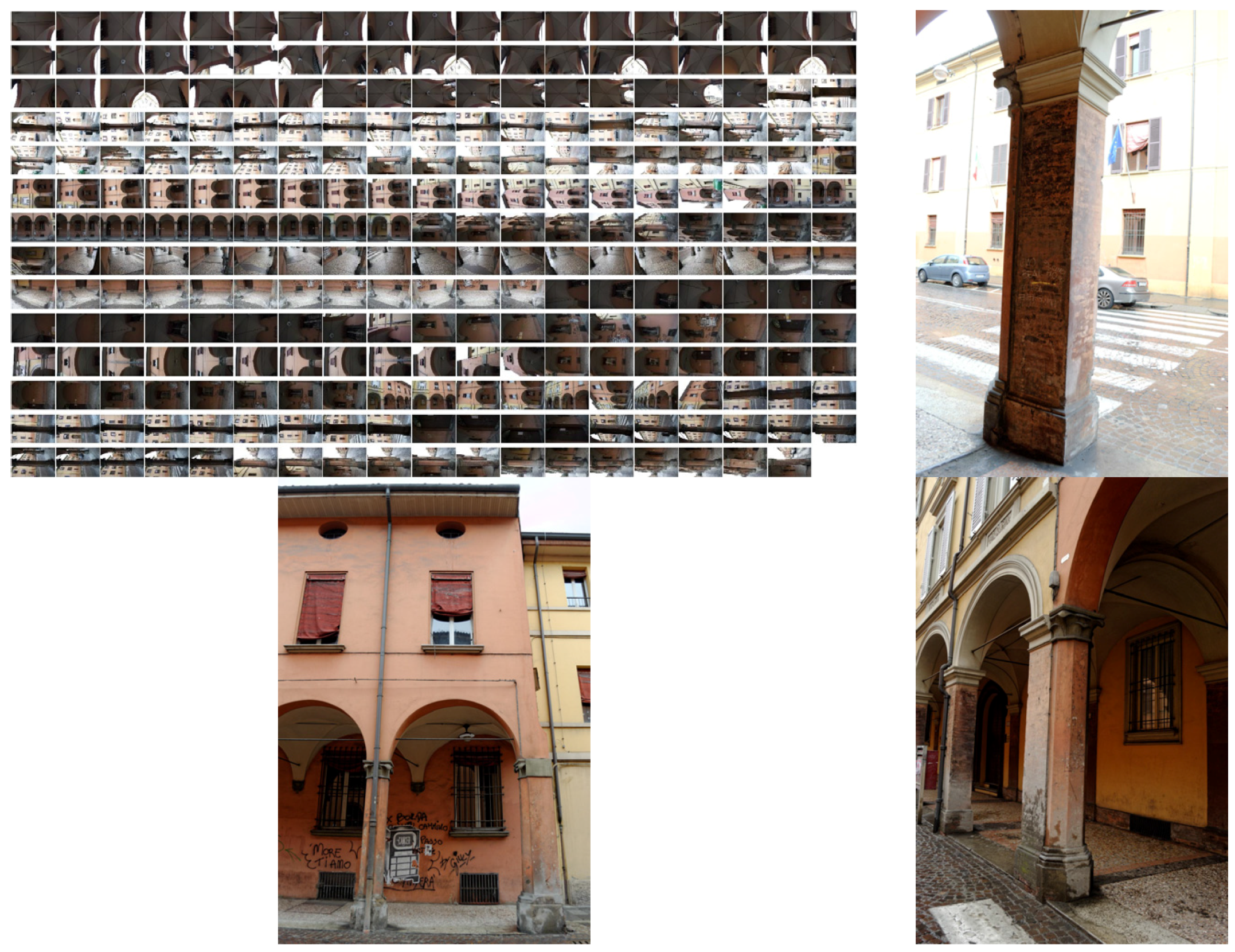
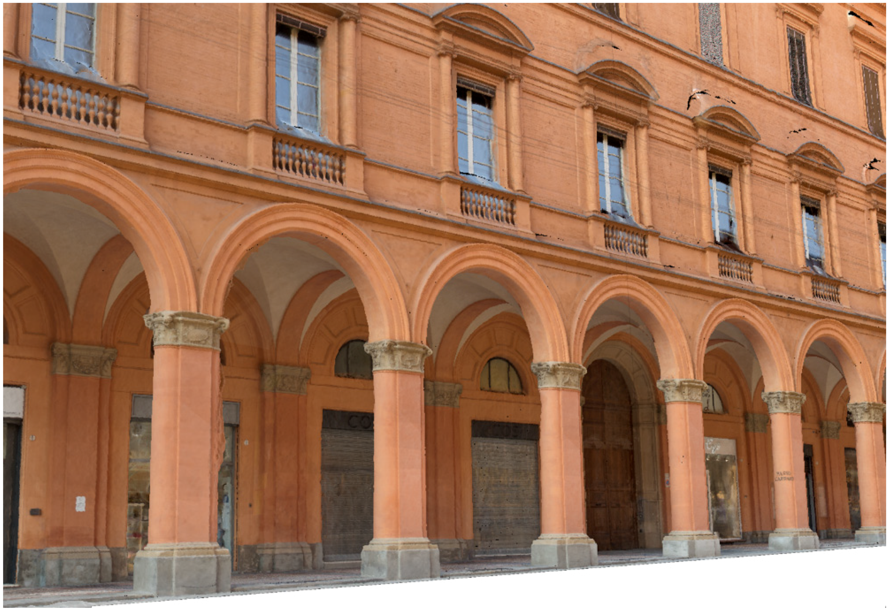
6.3. Dataset 3
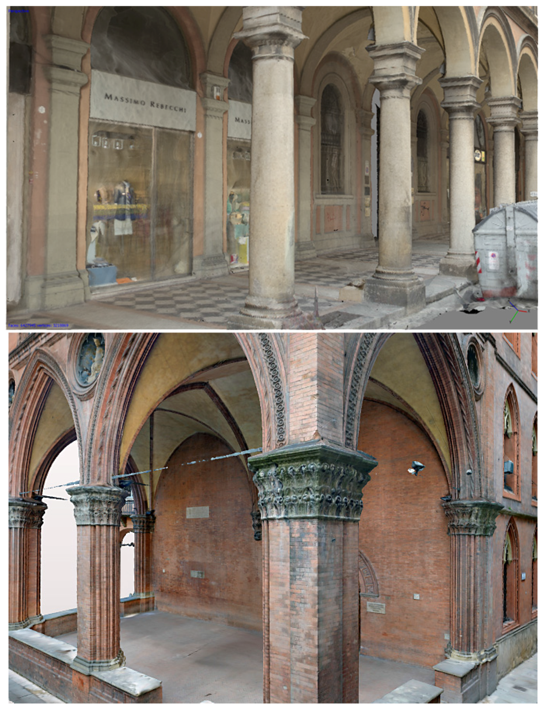
The last dataset (265 images acquired with a Nikon D3100, sensor size 23.1 × 15.4 mm, 18 mm nominal focal length) regards a three floors historical building (19 m height × 10 m width), characterized by arcades with four arches, columns, cross vaults and plastered walls with uniform texture. The camera was moved along the porticoes, with some closer shots of the columns and of the vaults (
Figure 13). The dataset is used to show how the various steps of the proposed pre-processing pipeline positively influence the 3D reconstruction procedure.
Table 7 reports the achieved image orientation results without and with pre-processing. The developed methods (
CBM3D-new for the noise reduction and
BID for the color-to-gray conversion) allow orienting larger numbers of images.
The dense matching procedure is then applied starting from the orientation results achieved in Photoscan results (
Table 8). In this case, it is also shown how an appropriate pre-processing procedure allows deriving denser point clouds. The point density distribution for the different dense clouds (named Local Density Computation) was estimated. The density has been computed using a tool able to count, for each 3D point of the cloud, the number of neighbors N (inside a sphere of a radius R, fixed at 20 cm). The results of the Local Density Computation (shown as color-coded maps and histograms) show that the successive combination of the proposed pre-processing methods gradually achieve, beside an increasing amount of 3D points, a higher density and a more uniform distribution of points.
7. Conclusions
The paper reported a pre-processing methodology to improve the results of the automated photogrammetric pipeline for 3D scene reconstruction. The developed pipeline consists of color balancing, image denoising, color-to-gray conversion and image content enrichment. Two new methods for image denoising (
CBM3D-new) and grayscale reduction (
BID) were also presented. The pipeline was evaluated using some datasets of architectural scenarios and advantages were reported. From the results in
Section 6, it is clear that the pre-processing procedure, which requires very limited processing time, generally positively influences the performances of the orientation and dense matching algorithms. The evaluation shows how the combination of the various methods is indeed helping in achieving complete orientation results, sometimes better BA re-projection errors (although it is not a real measure of better quality) and, above all, denser and complete 3D dense point clouds.
As shown in the results, the best strategy implies applying a color enhancement, a denoise procedure based on the CBM3D-new method, the BID method for grayscale conversion and the Wallis filtering. This latter filtering seems to be fundamental also in the orientation procedure and not only when applying dense matching algorithms (as reported in the literature).
The developed pre-processing method is quite flexible and features the following characteristics.
It is derived from many experiments and merging various state-of-the-art methods.
The setting parameters can be fixed reading the image metadata (EXIF header).
The denoising and grayscale conversion consider the entire dataset and they are not image-dependent.
It is customized for improving the automated 3D reconstruction procedure.
It is not based only on perceptual criteria typically used in image enhancement algorithms.
It also gives advantages to the texture mapping phase.
The presented research substantially improved our 3D reconstruction pipeline and allows us to model large architectural scenarios for documentation, conservation and communication purposes (
Figure 14).


