Corn Response to Climate Stress Detected with Satellite-Based NDVI Time Series

Abstract

Corn growth conditions and yield are closely dependent on climate variability. Leaf growth, measured as the leaf area index, can be used to identify changes in crop growth in response to climate stress. This research was conducted to capture patterns of spatial and temporal corn leaf growth under climate stress for the St. Joseph River watershed, in northeastern Indiana. Leaf growth is represented by the Normalized Difference Vegetative Index (NDVI) retrieved from multiple years (2000–2010) of Landsat 5 TM images. By comparing NDVI values for individual image dates with the derived normal curve, the response of crop growth to environmental factors is quantified as NDVI residuals. Regression analysis revealed a significant relationship between yield and NDVI residual during the pre-silking period, indicating that NDVI residuals reflect crop stress in the early growing period that impacts yield. Both the mean NDVI residuals and the percentage of image pixels where corn was under stress (risky pixel rate) are significantly correlated with water stress. Dry weather is prone to hamper potential crop growth, with stress affecting most of the observed corn pixels in the area. Oversupply of rainfall at the end of the growing season was not found to have a measurable effect on crop growth, while above normal precipitation earlier in the growing season reduces the risk of yield loss at the watershed scale. The spatial extent of stress is much lower when precipitation is above normal than under dry conditions, masking the impact of small areas of yield loss at the watershed scale.

1. Introduction

Crop yield in the US Corn Belt is strongly affected by climate variability, primarily through the influence of climate on water availability as soil moisture. The summer warming trend from 1891–1936 adversely affected crop yields, while a cooling trend accompanied by increased summer rainfall decreased variability in yield and accounted for a 20% increase in yield from 1936–1972 [1]. Crop yields during the period of 1980–2007 were strongly correlated with the occurrence of meteorological drought and maximum daily temperature during the grain filling and reproductive growth period [2,3]. Soil moisture that is either higher or lower than normal conditions can cause crop water stresses, which are harmful for crop growth over shorter spatial and temporal scales.

Despite clear evidence that soil moisture conditions cause billions of dollars of crop loss per year, the impact of water stress on crop growth is difficult to quantify. In part this is because the extreme events that cause yield loss are by definition infrequent in nature. Field-scale studies designed to investigate the impact of water stress must use artificial manipulation of moisture conditions [4,5] or they will far exceed the typical lifetime of a research grant. The available regional datasets are too coarse in spatial resolution. For example, the USDA National Agricultural Statistics Service’s (NASS) Crop Progress and Condition data is compiled at the state or sub-state level. Such datasets can capture the effects of region-wide environmental impacts such as drought, but events that are frequent at small scales (i.e., flooding in the field low spot) are particularly hard to detect due to the coarse nature of the datasets.

Corn phenology, the timing of corn growth and development each year, is weather and hybrid specific. For the same corn hybrid under similar management practices, growth conditions are strongly related with climate variability. When the hydroclimate is suitable, corn develops well and has higher yield potential, but when faced with biophysical stresses related to climate extremes many aspects of crop development can be affected. Observations related to the spatial variability in crop development can give insights into crop response to hydroclimate factors because of the spatial variability in soil water conditions, reducing the need for multi-year studies.

Analyzing corn phenology using remotely sensed satellite image provides an opportunity to investigate the linkage between the spatial variability in crop development and water stresses. Satellite data are increasingly used to monitor agricultural fields [6,7] and can provide a powerful tool to record phenological trends and detect the effect of climate variability. Compared to hand-held optical sensors, satellite images offer a valuable perspective at the field-scale instead of individual plants, revealing regional crop conditions that are difficult to detect from limited ground measurements. On the other hand, compared to coarse state level crop statistical reports, remote sensing imagery reveals substantially more about the spatial variability of corn development within a region. An additional benefit of satellite imagery is that data can be collected and processed in a repeatable and non-biased method. Additionally, spatial information, such as soil moisture from satellite images, can also be merged into crop modeling studies for improving regional crop yield forecasts [8,9].

Interest in studying crop phenology using satellite data has been growing in recent research [10]. Crops exhibit different features as they develop, many of these features are distinguishable from remote sensing imagery. For example, the area of green leaves associated with a plant strongly absorbs wavelengths of visible (red) light while reflecting near-infrared wavelengths [11]. The ratio of absorption to reflectance also varies from the early growing season through to maturity and senescence. Such changes in spectral properties are the theoretical basis for relating reflected radiation from satellite images to crop growth [12]. Vegetation indices are more widely used than reflectance in remote sensing algorithms for monitoring crop characteristics [13,14] because of their simplicity and the ease of data processing. A vegetation index is an indicator that describes a visible characteristic, for example, the greenness of a plant, which is correlated with the health of the vegetation. One widely used vegetation index is the Normalized Difference Vegetative Index (NDVI), which has been related to nitrogen status and chlorophyll content at micro scale and biomass, leaf area and grain yield at macro scale [15,16,17,18].

NDVI generated from remote sensing can be used to estimate crop growth under various climate conditions, which in turn can be used to improve and evaluate crop models [19,20]. Constructing time series of vegetation indices, such as NDVI, from satellite imagery can also help in the development of region specific phenologies for multiple crop types while limiting the necessity of intensive field monitoring. By merging NDVI values for the same region over multiple years, researchers can also establish “normal” growing conditions in a region for a specific time of year. Then by studying significant deviations from this “normal” phenological curve within any year, changes to crop phenology due to climate stresses can be quantified.

The overarching goal of this study is to evaluate variability in corn growth conditions and phenology both spatially and temporally in the St. Joseph River watershed, which is located in the Eastern Corn Belt, USA using an 11-year time series of Landsat 5 TM imagery. Corn growth conditions were identified using NDVI values from multiple years of satellite images, and linked with climate stresses and county level yield observations. By quantifying the variability in corn growth response in the presence of water stress, the phenologies extracted from the satellite data can be used to evaluate the ability of current generation crop growth models to represent plant responses to the more frequent occurrence of weather extremes under projections of climate change in the Corn Belt.

2. Materials and Methods

2.1. Study Area

The St. Joseph River watershed (Figure 1) with a drainage area of 2821 km² is located in northeastern Indiana, northwestern Ohio and southeastern Michigan. This watershed spans portions of eight counties. Agricultural land, including row crops and pasture occupy 67% of the basin area. Rainfed agriculture is predominant in the region, and just 5% of the cropland in the eight county area is irrigated [21]. Three NOAA weather stations recording daily air temperature and precipitation are located in Steuben, IN, Williams, OH and DeKalb, IN. The watershed is fully contained in a single Landsat 5 scene (path 21, row 31).

2.2. Data

2.2.1. Land Cover and Crop Progress Data

The Cropland Data Layer (CDL) product is a raster-formatted, geo-referenced, crop-specific, land cover map produced by the USDA National Agricultural Statistics Service (NASS). The purpose of the CDL program is to use satellite imagery to provide acreage estimates of major crop commodities for each state [22]. The resolution for CDL products is 30 m, so the area of each pixel is 900 m². The CDL is available for Indiana beginning from 1999, and for Ohio and Michigan from 2006 and 2007, respectively. The CDL products are used to identify corn pixels in the St. Joseph River watershed for each year of analysis. These are in turn used to extract the spectral signature (NDVI) for corn only, which is the focus of this study.

USDA/NASS releases basic phenological information for corn in weekly Crop Progress and Condition Reports at the state or agricultural statistic district level [23]. The latter is a sub-state region comprised of multiple counties. These reports show the percent of crop fields (by area) that have reached or completed a specific phenological stage (planted, emerged, silking, dough, dent, mature and harvested) each week during the growing season. The weekly progress reports were used to identify the range and median in growing season length in the Northwest District of Indiana using the dates for corn planting and harvesting each year. Ohio and Michigan do not report district level crop progress data, so information from those states were not used for defining the growing season.

2.2.2. Remote Sensing Observations

Eleven years of Landsat-5 Thematic Mapper (TM) images (Path 21, Row 31) were downloaded from the USGS EarthExplorer [24] for the duration of the CDL data in the St. Joseph River watershed (2000–2010). The resolution of the Landsat 5 TM image pixel is 30 m × 30 m. The Landsat satellite collects images for the same location every 16 days, so there are approximately 10 images spanning the corn growing season each year. Only images with cloud coverage less than 60% were kept for analysis.

Table 1. Selected Landsat TM5 images during the growing season, path 21, row 31.

Year	Date	Day of Year	Cloud Coverage (%)	Year	Date	Day of Year	Cloud Coverage (%)
2000	27 April *	118	0	2005	9 April *	99	0
	13 May	134	0		27 May	147	23
	29 May	150	0		30 July	211	19
	14 June	166	30		18 October	291	0
	30 June	182	10	2006	28 April *	118	0
	2 September	246	20		15 June	166	7
	18 September	262	0		1 July	182	21
	20 October	294	0		17 July	198	0
2001	30 April *	120	0		2 August	214	1
	17 June	168	0		5 October	278	12
	4 August	216	0	2007	15 April *	105	0
	20 August	232	10		1 May *	121	49
	5 September	248	0		18 June	169	4
	7 October	280	10		20 July	201	0
2002	3 May *	123	0		22 September	265	0
	20 June	171	0	2008	3 May *	124	22
	6 July	187	0		20 June	172	37
	22 July	203	30		6 July	188	2
	7 August	219	0		23 August	236	10
	8 September	251	0		24 September	268	0
	24 September	267	0		10 October	284	0
2003	6 May	126	30	2009	4 April *	94	13
	22 May	142	0		22 May*	142	17
	23 June	174	0		23 June	174	3
	25 July	206	3		9 July	190	7
	11 September	254	0		11 September	254	5
	27 September	270	14	2010	9 May	129	13
	13 October	286	0		10 June	161	0
2004					26 June	177	23
	8 May	129	60		29 August	241	3
	25 June	177	22		14 September	257	0
	13 September	257	4		30 September	273	10

* Image date is earlier than the USDA National Agricultural Statistics Service’s (NASS) recorded date for 50% of planting completed.

lists the 63 Landsat 5 TM images used for this analysis with their acquisition dates and cloud coverage.

2.3. Data Processing

The NDVI is developed from two important wave bands: the red and near infrared, and has been widely used for agricultural mapping and yield monitoring [25,26,27,28,29]. The NDVI is calculated as:

$$NDVI=\raisebox{1ex}{$\left(R_{NIR}-R_{red}\right)$}\!\left/ \!\raisebox{-1ex}{$\left(R_{NIR}+R_{red}\right)$}\right.$$

(1)

where R_nir is the reflectance in the near infrared spectrum, and R_red is the reflectance in the red band spectrum. Values of NDVI range from 1.0 to −1.0 [30]. Barren land, sand or snow usually present very low NDVI values (for example, less than 0.1). Sparse vegetation such as shrubs and grassland or senescing crops may result in moderate NDVI values (approximately 0.2 to 0.5). High NDVI values (approximately 0.6 to 0.9) correspond to dense vegetation such as that found in temperate and tropical forests or crops at their peak growth stage. Since the NDVI shows a close relation to canopy chlorophyll content, it can also be used to estimate Leaf Area Index (LAI) [31,32], which is an important vegetation biophysical characteristic.

NDVI values also change during the plant growing cycle. During development from planting to physiological maturity, corn experiences several growth stages. These stages are separated into two groups: vegetative and reproductive periods. The vegetative period covers the timing from planting to the stage when the entire tassel is visible (the visible tassel or VT period) and leaves are fully developed. The reproductive period starts from the silking stage and ends at physiological maturity. For a single plant, the growth rate is slow at the beginning of the vegetative period, but increases when new leaves appear. It reaches the maximum canopy coverage in the early reproductive period. Corn NDVI values roughly follow the same trend, where the peak NDVI value is often observed during the silking period. Natural senescence usually begins at the end of the denting period; NDVI values decrease from the beginning of natural senescence to maturity.

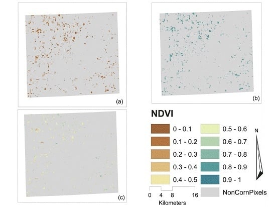
2.3.1. NDVI Calculation for Corn Pixels

The first step for computing NDVI values for corn pixels is to remove non-clear land pixels for all Landsat TM5 images. The object-based cloud and cloud shadow detection software Fmask [33] was utilized to identify cloud, shadow and unobstructed land surface pixels. Digital Number values from the visible and near-infrared bands in the raw Landsat 5 TM imagery are first converted to Top of Atmosphere (TOA) reflectance, while the thermal band is converted to Brightness Temperature (BT) using the Landsat Ecosystem Disturbance Adaptive Processing System (LEDAPS) [34]). The TOA reflectance and BT (in degrees Celsius) are used as Fmask input. Decision rules based on cloud and cloud shadow physical properties (brightness and temperature) are then used to extract a potential cloud/shadow layer. Cloud potential layers are improved by eliminating edge cells. Then the base and top height of clouds are computed and used to calculate projected shadows. Shadow detection is refined via a shape similarity comparison, where geometric relationships are used to match the potential cloud shadow with the cloud. Clearly visible land pixels are identified by Fmask as those with data that are not covered by cloud, cloud shadow or snow. Pixels used for the analysis are further screened to make sure that they are clearly visible for every Landsat image for a specific year by merging the Fmask products for all TM images in each year. As corn is not grown consistently on the same fields on a year-to-year basis (as defined by local crop rotation practices), the pixels selected for analysis did vary between years.

The final outputs of Fmask are clear land pixels for all TM5 images in each year. Quick Atmospheric Correction (QUAC) from Exelis ENVI was used to remove the effects of the atmosphere on the reflectance values of all clear land pixels. QUAC determines atmospheric correction parameters using an in-scene approach without ancillary information, requiring only specification of sensor band locations and their radiometric calibration [35]. The final product for NDVI calculation after running QUAC was reflectance from all clear land surface pixels.

NDVI for all land pixels was calculated based on the atmospherically corrected reflectance of band 3 (red, 630–690 nm) and band 4 (near infrared, 760–900 nm). Pixels identified as corn in each CDL data layer from 2000–2010 are used to extract the corn NDVI values for pixels within 15 km of the St. Joseph River watershed. The purpose of extending the selection area to include areas outside the watershed is to enlarge the sample size for corn pixels. It is assumed that growing conditions within the 15 km buffer are similar to the ones inside the watershed boundary.

Three additional filters are applied to further refine the selection of corn pixels identified by the CDL data, to minimize the potential for mixed pixels and registration errors that can introduce noise into the data. The first filter improves the identification of pure corn pixels by removing any pixel that had more than one non-corn neighbor. These are assumed to be edge-of-field pixels with a greater likelihood of being mixed. The second filter checks for a minimum amount of change in NDVI between planting and silking when NDVI should peak., Here the median NDVI value for all corn pixels was calculated for all images for a year, and the image with the peak median NDVI (near silking stage) and minimum NDVI (near planting) were identified. The difference between median NDVI for those two images was set as a threshold. Any pixel with maximum NDVI range less than that threshold over all images in the year was excluded. The final filter checks that NDVI increased monotonically from planting date to peak NDVI stage, then decreased monotonically from peak stage to maturity stage. Due to the limited availability of images each year, the maximum NDVI value calculated from the Landsat images may not always be the peak NDVI for that year. It is possible to have a non-monotonic change for valid pixels if the peak growth period is missed due to the lack of available imagery. Therefore, the monotonic check is applied for images between the latest planting date and earliest silking date, and images between the latest silking date and earliest maturity date, where these dates have been extracted from the USDA NASS Crop Progress Reports (

Table 2. NASS corn progress dates for the St. Joseph River Basin.

Crop Status	Year	Day of Year Status Begin	Day of Year Status End	50% Progress Status
Planted	2000	107	156	127
	2001	105	147	124
	2002	111	167	145
	2003	110	159	122
	2004	109	151	119
	2005	100	142	122
	2006	106	155	123
	2007	112	147	130
	2008	118	167	130
	2009	123	165	143
	2010	106	155	126
Silked	2000	184	219	200
	2001	196	217	201
	2002	195	223	206
	2003	194	229	207
	2004	179	221	192
	2005	191	219	199
	2006	190	218	199
	2007	189	217	197
	2008	195	230	205
	2009	193	228	208
	2010	183	218	199
Matured	2000	240	282	263
	2001	238	287	263
	2002	244	286	268
	2003	250	285	273
	2004	242	291	262
	2005	233	289	263
	2006	239	288	267
	2007	245	287	263
	2008	251	300	265
	2009	256	312	286
	2010	239	281	262

). Since 2004 had only three available images, the third filter was not applied. Figure 2 illustrates the impacts on NDVI after each of these filters.

2.3.2. Normal Curve Generalization and NDVI Residual Calculation

Since corn phenology is more correlated with air temperature (or heat units) than Julian days since planting, development varies from year to year with respect to date [36]. Therefore, the extracted NDVI data are associated with the Potential Heat Units (PHU) and Growing Degree Days (GDD) accumulated from the planting date to the date of image acquisition. PHU and GDD are both used as measures of the growth and development of plants based on daily average temperature. PHU is calculated based on degrees Centigrade, while GDD is based on degrees Fahrenheit. Development does not occur unless the daily average temperature is above a base temperature (lower limit). PHU/GDD start to accumulate from the planting date to the date of physical maturity for the plant as long as temperature is above the lower limit. The lower limit for corn is set as 8 °C [37]. The GDD method also has an upper limit, which is set to 86 °F/30 °C [38], representing temperature above which the crop is too stressed to continue development towards maturity. Such a limit does not exist with the PHU.

A generalized corn NDVI growth curve is obtained using a robust version of LOESS (locally-weighted scatter plot smoothing) [39] applied to median NDVI values from all 11 years’ images plotted vs. PHU and GDD. Due to data scarcity (3–7 images per year) and the timing difference of images, it is hard to describe the corn NDVI dynamics for specific growth periods using just one year’s data. Therefore, all years of data are combined to create a general, regional corn growth curve. In this way, missing information for a specific period in one year can be compensated by other years. The generalized NDVI curve via local regression method reflects the corn growth dynamics under “normal conditions” for 11 years. The differences between measured NDVI and the derived normal curve, the residual or “discrepancy score” [40], can be treated as an index to reflect the influence of biophysical stresses on crop growth. If the residual has a negative value, corn development is below normal so can be assumed to have experienced more growth stress than in a normal year. The Sakamoto et al. [40] “discrepancy score” was computed based on a rescaled shaped model from 7 years of continuous daily MODIS data and smoothed for each year. Therefore, their “discrepancy score” differs for each year, which is different from our image based residuals. By comparing the median NDVI for a specific image and the normal curve, we can roughly estimate basin level corn growth condition in a specific day. Interannual corn growth analysis can be conducted by averaging NDVI residuals based on satellite imagery. To obtain the spatial growth variability, the departure rate can also be computed based on NDVI and the normal curve for each individual pixel.

2.3.3. Growth Stress Metrics

Actual crop growth is affected by various stresses occurring during the growing season, including those from extreme temperatures, oversupplied or limited water, insufficient nutrients, pest infestations, and weed competition. Actual growth is therefore always less than or equal to the potential growth even under optimal conditions.

In this research, only crop growth stresses from extremes of temperature and water, based on the approach used in the Soil and Water Assessment Tool (SWAT) were calculated [41].

Daily temperature stress (ts) is calculated as:

$$ts=1 Tav>2*Topt-Tbase or Tav\le Tbase$$

(2)

$$ts=1-\exp \left[\frac{-0.1054*{\left(Topt-Tav\right)}^2}{{\left(Tav-Tbase\right)}^2}\right] Tbase<Tav<Topt$$

(3)

$$ts=1-\exp \left[\frac{-0.1054*{\left(Topt-Tav\right)}^2}{{\left(2*Topt-Tav-Tbase\right)}^2}\right] Topt<Tav<2*Topt-Tbase$$

(4)

where Tav is the mean air temperature for day (°C), Tbase is the plant’s base or minimum temperature for growth (°C) (defined as 8 °C for corn), and Topt is the plant’s optimal temperature for growth (°C) (defined as 25 °C for corn).

Accumulated temperature stresses normalized by the number of days or heat units are used to quantify the cumulative effect of temperature on crop growth.

$$t{s}_{acc\_day}=\frac{{{\displaystyle \sum }}_i^{n}ts}{n-i}$$

(5)

$$t{s}_{acc\_PHU}=\frac{{{\displaystyle \sum }}_i^{n}ts}{{{\displaystyle \sum }}_{i=1}^{n}PHU}$$

(6)

$$t{s}_{acc\_GDD}=\frac{{{\displaystyle \sum }}_i^{n}ts}{{{\displaystyle \sum }}_{i=1}^{n}GDD}$$

(7)

where ts_{acc_day} is the accumulated temperature stress normalized by the number of days from planting date i to image collection date n; ts is daily temperature stress; ts_{acc_PHU} is the accumulated temperature stress normalized by PHU; PHU is the accumulated heat units from day i to day n; ts_{acc_GDD} is the accumulated temperature stress normalized by GDD; GDD is the accumulated growing degree days from day i to day n.

Water stress (ws) is computed based on the difference between average accumulated rainfall from long term historical data and accumulated rainfall for each year, as follows:

$$ws={{\displaystyle \sum }}_{i=1}^n{p}_i-{{\displaystyle \sum }}_{i=1}^n\overline{p_i}$$

(8)

where p_i represents daily precipitation for a single year and p_i is the daily normal precipitation for a 20 year period (1991–2010). ws is calculated by comparing the accumulation of precipitation from the average curve $({\displaystyle \sum }_{i=1}^n\overline{p)}$ with that for the current year (${\displaystyle \sum }_{i=1}^{n}p$) relative to the planting date i for the year of interest, and can be calculated to any day n in that year. If ws is a negative value, it means the accumulated rainfall amount is below the average condition, so corn at that time may have suffered more from drought. On the other hand, if ws is a positive value, it indicates a wetter than average condition. As shown in Figure 3, the cumulative rainfall curve for year 2002 is below the long term average curve, which results in negative ws values in this dry year. Positive ws values are found for the year 2003, indicating it was wetter than average. Year 2006 is normal year, because the accumulation of precipitation in 2006 is close to the long term average.

3. Results

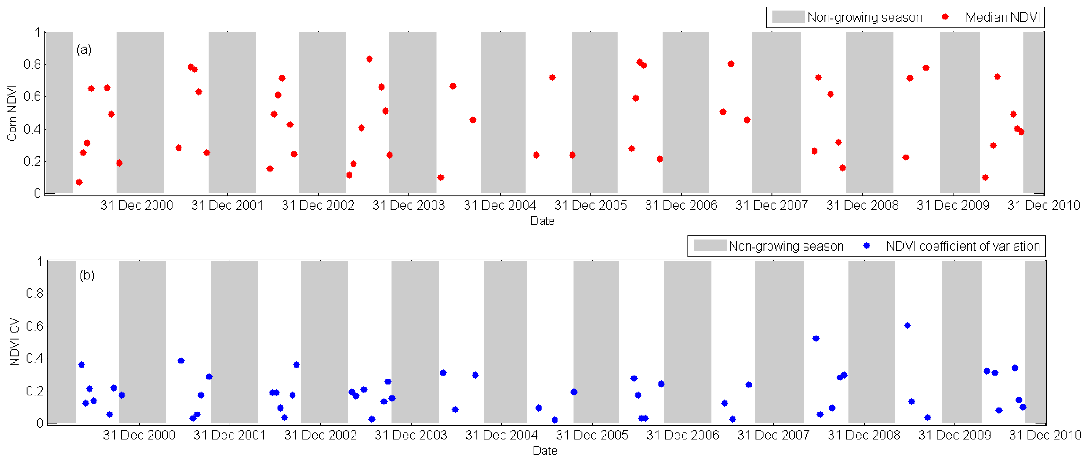
3.1. Normalized Difference Vegetative Index with Time

Figure 4a illustrates the median growing season corn NDVI values for 11 years of images (2000–2010). The median value of corn NDVI follows the expected phenology of the corn canopy. In the early growing period, as corn plants emerge, vegetation coverage per unit area is small, and the median NDVI value is low (0–0.2). As plants develop, the NDVI value grows rapidly (0.3–0.6) capturing the increase in leaf area as the growing plant spreads to cover the soil between the rows in the fields. The NDVI value is proportional to the canopy coverage during this stage. Corn NDVI reaches a peak value (0.7–0.8) at the end of July or early August, at the stage when all leaves are fully developed. As plants enter the end of the reproductive stage and natural senescence occurs, NDVI decreases significantly.

Figure 4b shows the Coefficient of Variation (CV) of corn NDVI with time. Minimum CVs for each year are found in the middle of the growing season associated with the peak NDVI value. This period appears to be the most uniform stage, when the corn canopy is fully developed and spatial differences due to different planting dates are less pronounced. Peak CVs are often encountered either at the early or late growing season. In the early growing season when corn is just emerging, soil reflectance dominates the NDVI measurement, causing a very low mean NDVI value (e.g., Year 2000, 2003 and 2010), and therefore a higher CV. Secondly, due to different planting dates, NDVI values show greater variance in late June (around 30–40 days after planting), leading to higher CV values (Year 2001, 2008 and 2009). In the late growing season, as senescence occurs, the reflectance contains a wide range of green and non-green color intensities, also causing high CV values.

Table 3. Date of maximum NDVI variation (range of the 95% prediction interval) for each year.

Date	Days after Planting	95% Interval	Median NDVI	CV
17 September 2000	133	0.4050	0.4938	0.2207
16 June 2001	43	0.4565	0.2833	0.3868
5 July 2002	41	0.3561	0.4934	0.1875
26 September 2003	147	0.4677	0.5117	0.2605
12 September 2004	136	0.5128	0.4591	0.2974
17 October 2005	168	0.1535	0.2387	0.1937
30 June 2006	58	0.3870	0.5906	0.1728
21 September 2007	134	0.4343	0.4588	0.2368
19 June 2008	40	0.5690	0.2665	0.5225
22 June 2009	30	0.5841	0.2253	0.6017
28 August 2010	114	0.5783	0.4930	0.3415

lists the date of the maximum NDVI variation for each year. Those dates are always found during either the leaf development stage or senescence period. This spatial variability in NDVI is illustrated in Figure 5 for De Kalb County in the year 2003. The spatial distribution pattern on 27 September appears more heterogeneous than on 25 July, when canopy coverage and leaf overlap were well-developed.

3.2. Normal Growth Condition

The generalized corn NDVI growth curve obtained from all 11 years’ images is shown in Figure 6. Since different planting dates each year may affect the starting point of the NDVI curve, the NASS recorded planting date (50th percentile value) is used as the starting point for each year’s analysis. In addition, different lengths of the growing season (number of days vary from 122 days in 2002 to 151 days in 2003 based on the 50th percentile of NASS crop progress records) may make it difficult to identify NDVI values for a specific growing period defined by Julian days. Therefore, NDVI dynamics are also regressed against PHU and GDD accumulated from the planting date (Figure 6). Two outliers (see Figure 6) were removed when generating the normal growth curve. The first is from 2005 imagery, and is removed because it associated with an extremely high PHU and GDD suggesting that it was collected well after crop maturity. The second one is from 2007 imagery, and yields extremely high NDVI values at the very end of the growing season, suggesting the NDVI value at this time does not correctly represent the corn growth condition.

The departure of image median NDVI values from the normal curve (NDVI residual) are calculated and plotted vs. Julian days, PHU and GDD, respectively (Figure 7). For year 2002, most NDVI residuals are negative, indicating increased stress levels relative to the long-term average for almost the entire growing season, which can be attributed to the drought that occurred that year. For years 2008 and 2010, corn NDVI deviations are negative for the second half of the growing season, suggesting increased stress on crop growth in the later parts of the growing season. Years 2004, 2007 and 2009 all have positive residuals during the peak NDVI stage, indicating corn growth is above normal. Residuals for the other years are small so NDVI values are close to the normal curve, indicating an average growth year. Corn response to year to year variability is reflected in these departures from the normal curve. Therefore, positive NDVI residuals do not necessarily mean the corn is not in any way stressed, but that its growth is above the normal condition based on the multiple year record.

The rank of the annual discrepancy score (average of the residual calculated for each image over a growing season) is summarized in

Table 4. Rank of NDVI residual for each set of annual images. Rank 1 = best NDVIs, while Rank 11 = worst NDVIs.

	Days		PHU		GDD		Growing Season Rainfall Amount (mm)	Growing Season Mean Temperature (°C)
Year	Rank	Discrep. Score	Rank	Discrep. Score	Rank	Discrep. Score
2000	4	0.0171	6	0.0090	6	0.0041	482	19.6
2001	6	−0.0019	4	0.0275	3	0.0301	460	19.9
2002	11	−0.1086	11	−0.0797	11	−0.0667	390	20.2
2003	3	0.0391	3	0.0407	2	0.0317	634	19.7
2004	5	0.0100	7	0.0054	7	0.0034	445	19.9
2005	8	−0.0183	5	0.0225	5	0.0262	287	21.6
2006	9	−0.0399	9	0.0011	8	0.0026	384	20.8
2007	2	0.1069	2	0.0480	4	0.0282	378	20.8
2008	10	−0.0743	10	−0.0563	10	−0.0573	394	19.8
2009	1	0.1134	1	0.0542	1	0.0450	490	18.0
2010	7	−0.0028	8	0.0029	9	0.0008	358	19.7

. High rankings indicate positive residuals, meaning that the crop experienced higher NDVI than normal conditions, while low rankings indicate that crop experienced lower NDVI than normal conditions. Although there is some variation in ranks based on whether Julian days or heat units are used, the relative positions in the rankings are quite consistent. For example, 2002 and 2008 are always the lowest ranked years, while 2009 and 2003 are more highly ranked regardless of the independent variable. The annual yield for 2002 and 2008 was 6.65 and 8.03 t/ha, which are around 1.50–3.00 t/ha lower than year 2003 and 2009 (9.51 and 9.48 t/ha respectively), confirming that corn in 2002 and 2008 may have experienced more growth stress, which negatively affected yield.

3.3. Yield-NDVI Residual Relationship

Biophysical stress at different crop growth stages produces different magnitudes of influence on final yields [42,43]. Therefore, the relationship between NDVI residuals averaged over various growth stages and county level corn yields was investigated. Growth stages selected for analysis include: (1) The pre-silking period, where average NDVI residuals are calculated based on all available images from planting to the earliest silking date recorded by NASS data (Table 2). Average NDVI residuals during this period should reflect the corn growth condition during the corn vegetative period. Stress in this period reduces stem and leaf cell expansion resulting in lower plant height and less leaf area [44]; (2) The pre-maturity period, where NDVI residuals are calculated based on available images from planting to the earliest maturity date recorded by NASS data. This period contains both the corn vegetative stage and the most important reproductive stages (silking, blister and dough) of the corn plant life cycle. Stress in the early and middle reproductive stages can abort kernels, reduce kernel weight, and increase lodging, and in turn impair final yield [45]; (3) The silking period, where the NDVI residual are calculated for the image with the highest NDVI value for each year. This image is typically found in the silking period, when the canopy is fully developed. Early season stresses affect leaf area development, leading to differences in maximum NDVI values for each year. The NDVI residual for this image is caused by accumulated stresses during the vegetative period, which could also affect final yield; (4) The whole growing period where average NDVI residuals are calculated based on all available images. This is the same as the annual discrepancy score introduced previously.

The relationship between these four NDVI residuals, calculated from the three different generalized growth curves, and annual yield are summarized in

Table 5. Pearson correlation coefficient, r, between grain yield and average NDVI residuals for different growth stages.

	Day		PHU		GDD
Mean NDVI departure for pre-silking period images	0.067		0.71 *		0.76 **
Mean NDVI departure for pre-maturity period images	0.16		0.58		0.62 *
Mean NDVI departure for all images in the growing period	0.50		0.68 *		0.69 *
Departure for Highest NDVI point for each year	0.28		0.36		0.36

* means significant correlated when p < 0.05, ** means significant correlated when p < 0.01.

. No significant relationship was found (for significance level, alpha = 0.05) for any period if Julian day is used to generate the normal curve. When PHU and GDD are used to generate the normal growth curve, a significant relationship exists between NDVI residual and corn yield for the pre-silking, pre-maturity and entire growth periods. For the pre-silking period, a significant relationship (p < 0.01) was detected between average NDVI residuals based on GDD and annual corn yield (Figure 8). Average NDVI in the pre-maturity stage (p < 0.05) and for the whole growing season (p < 0.05) were also statistically significant predictors of annual yield. No significant relationship was found between the residual of the maximum NDVI image and annual crop yield, for any of the three normal growth curves. The relationship between annual basin level corn yield and NDVI residuals at different growing stages (GDD based) are also shown in Figure 8.

The correlation analysis summarized in Table 5 indicates that the NDVI residual derived from Landsat images reflects crop stress in the pre-silking period that in turn impacts final yield. This result is consistent with other studies that have found that NDVI from the middle to late vegetative period is significantly correlated with biomass and final yield [46,47]. Therefore, it may be possible to predict corn grain yield in-season for this study area, by comparing pre-silking period NDVIs to long-term normal growth curves.

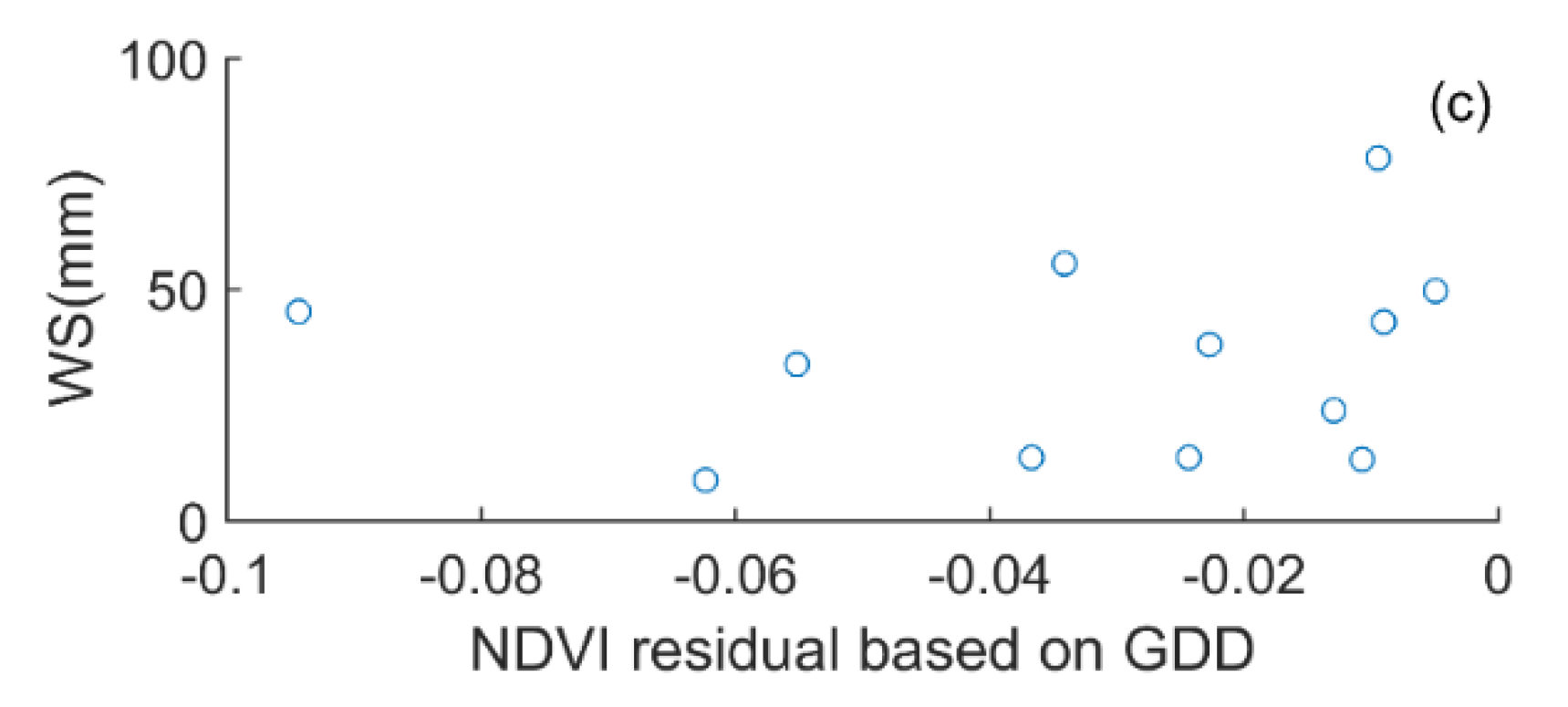
3.4. Stress-NDVI Residual Relationship

As stated in Section 3.3, annual corn yield is significantly related to the annual, pre-silking and pre-maturity NDVI discrepancy scores. The relationship between NDVI discrepancy and precipitation and temperature stress metrics are investigated in this section. The NDVI residuals calculated for all images in the 11-year period in Section 3.2 are grouped into pre-silking period, pre-maturity period and whole growing period. However, the residuals in those periods are not averaged as they were for the yield-residual relation, but rather regressed with normalized stress indices (ws and ts_acc) on the date of image acquisition.

The relationship between NDVI residuals and water stress (ws) is shown in Figure 9. Large negative values of water stress (ws) represent dry conditions; positive ws represent wet conditions. There are no strong correlations found in the data (Figure 9), but it appears that points can be grouped into several clusters. Image averages in Cluster A have both negative NDVI residual and water stress, which indicates that the weather is dry and crop growth is below normal. Cluster C has both positive NDVI residuals and water stress, so precipitation and crop growth are both above normal. Images in Cluster B represent normal weather and crop conditions. Compared to Cluster B both cluster A and C have relatively larger absolute values (0.2–0.4) in NDVI residuals, indicating larger growth discrepancies (could be either under or above normal condition). When corn growth is way above or below normal, it is usually associated with extreme climate conditions. Images in cluster B do not have a clear relationship between water stress and NDVI residuals. Since crop growth can be affected by many environmental factors, for example, soil types and slopes, temperature, disease and pests, leaf growth in this cluster may not respond to water stress exclusively, but is influenced by other environmental factors. Figure 9c also has a fourth cluster, named Cluster D, that contains images collected from the end of the growing season (after middle September) in 2003. Images in this cluster have very large positive ws values, but an unclear relationship between ws and NDVI residuals. This indicates that an oversupply of rainfall at the end of the growing season did not have a substantial effect on crop development. NDVI residuals at that time are more strongly related to the natural senescence process than water stress.

The relationship between NDVI residuals and normalized temperature stress indices (ts_acc) are summarized in

Table 6. Pearson correlation coefficient, r, between stress indices and NDVI residuals for different growth stages.

	Day	PHU	GDD
NDVI departure for pre-silking period images vs. Normalized accumulated temperature stresses	−0.36	0.32	0.42
NDVI departure for pre-maturity period images vs. Normalized accumulated temperature stresses	−0.18	0.32	0.35
NDVI departure for all images in growing period vs. Normalized accumulated temperature stresses	0.07	0.27	0.27

. No statistically significant relationship (p < 0.05) was found between temperature stress and NDVI residuals at any period based on either time units or heat units. This might be caused by the temperature stress calculation method. Compared to average daily temperature, daily maximum temperature is more associated with crop growth [3]. Leaf development is significantly affected by temperature when it is associated with water limitation. A more mechanistic analysis is needed to evaluate interactions between temperature, precipitation and other factors as they determine evapotranspiration, which is more closely related to NDVI [48].

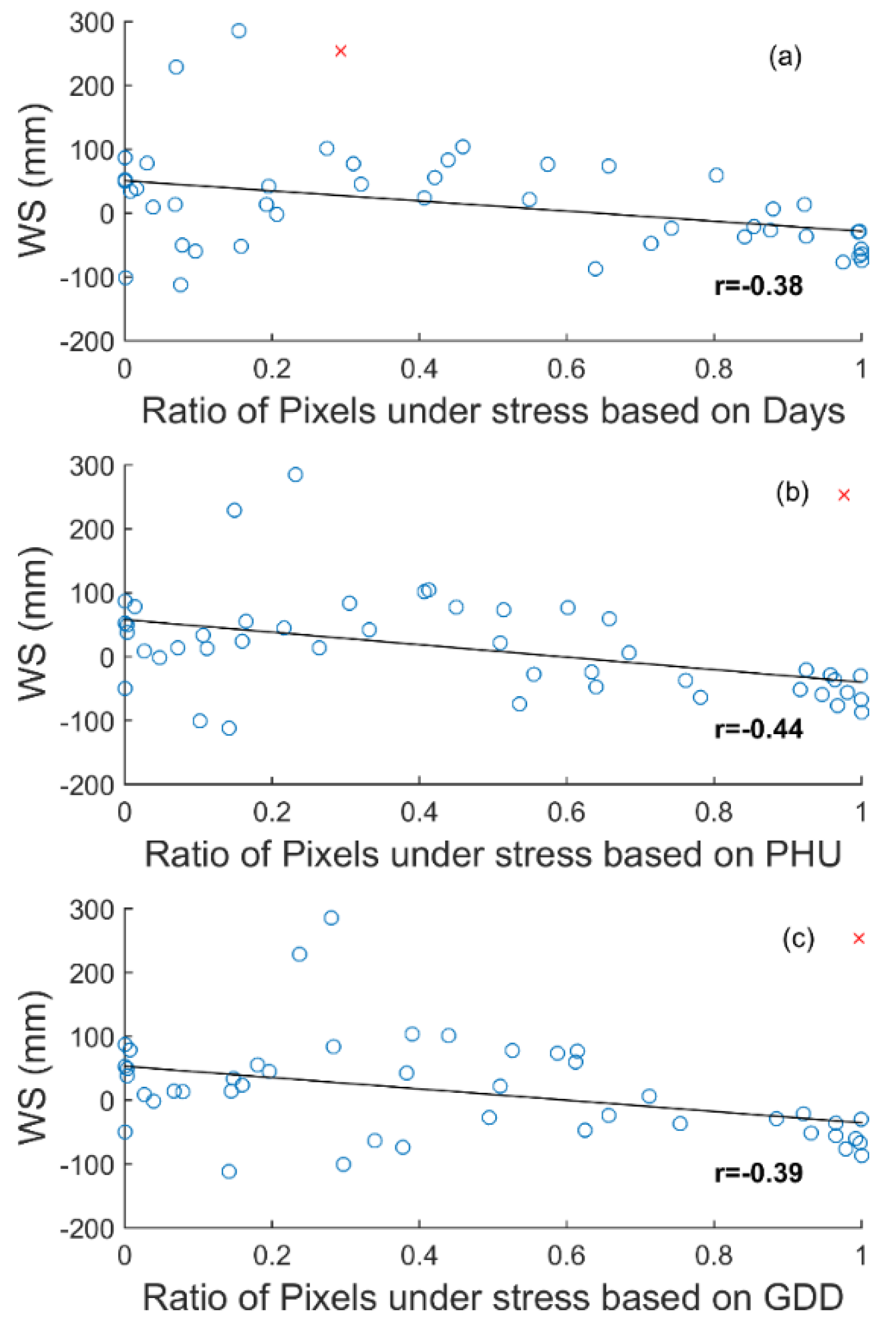
3.5. Risky Pixel Rate-Stress Realtionship

In Section 3.3 and Section 3.4, the relationship between image median NDVI residual and crop yield and climate metrics was investigated. Since NDVI residual was computed based on the image median NDVI value, the analysis neglected the spatial variability in crop stress. In this section, more emphasis is put on individual pixels under stress. Any corn pixel with NDVI less than the normal growth curve (Figure 6) is considered to be under stress. The percentage of pixels under stress (risky pixel rate) for each image is computed, and related to water stress (Figure 10).

Statistically significant relationships (p < 0.05) are detected between water stress and risky pixel rates, no matter which method was used to produce the normal growth curve. Therefore, the number of pixels experiencing growth limitations is strongly correlated with water stress. Based on Figure 10, images with risky pixel rates over 0.8 (80% of cells are under stress) have negative ws values, indicating drought condition is affecting crop growth for most cells. Almost all images with low risky pixel rate (less than 0.2) are associated with positive ws values, so above average rainfall reduced the threat of yield loss (less area experienced yield reduction). This difference in area affected under wet and dry stress is illustrated by comparing two images from the pre-silking stage for a dry year (2002) and a wet year (2003) (Figure 11), which clearly reflects the different impacts of rainfall on risky cell rates. If rainfall is limited, then most cells are under stress (Figure 11a). However, if rainfall is above average, only a small portion of cells are under stress (Figure 11b). This reflects the collection of runoff and ponding in depressional areas that may experience catastrophic yield loss, as opposed to the depressed growth over widespread areas in the case of water limitations.

For wet years, although fewer cells are affected by stress (risky pixel rate < 0.2), the potential yield loss in those cells with high stress rates could be huge. This is investigated using NDVI residuals that can represent potential yield, and ws, for risky cells (negative NDVI residuals) only when the risky pixel rate is less than 0.2, and ws > 0 (Figure 12). Though there is no clear relationship between ws and the NDVI residuals, in Figure 12a, we found that very large ws values (ws > 200 mm, both found in 2003) are always associated with large negative NDVI residuals, indicating potential yield loss in those cells. The overall yield in 2003 for the study area was the 3rd highest in the 11 year period (2000–2010), which means that yield losses in those few cells where water stress was high are compensated by increased yield in other cells that benefitted from sufficient rainfall.

4. Discussion

The information obtained from this study can be applied to three outcomes: (1) quantifying plant growth and environmental stress time series, which can be used to validate and constrain crop growth models; (2) improving early in-season yield prediction; and (3) identifying areas, which have the potential risk to obtain lower yields.

NDVI time series can provide important information for crop modeling studies by providing an additional, sub-annual time series for evaluating models. NDVI residuals can serve as the observed data to evaluate simulated leaf development responses to climate stresses. In most dynamic crop models, biomass and yield are a function of the daily predicted LAI. Understanding the LAI progression under stress and non-stress conditions is helpful to better estimate not only the annual yield but also interannual yield variation. Since LAI can be estimated from NDVI via various approaches [49,50], it is possible to adjust model predicted LAI based on NDVI from Landsat images and evaluate the accuracy of crop model performance in crop growth at different stages and under various climate stress conditions. This evaluation is especially important when exploring future climate change impacts. Crop modeling must be able to correctly reflect seasonal crop growth responses under various climate conditions (limited or oversupplied water). Validating crop growth model via information from this study can improve the reliability of model predictions under more frequent extreme weather in the future.

Results in Section 3.3 reflect a significant relationship between pre-silking stage NDVI residual and corn yield in the St. Joseph River Watershed. This indicates corn yield potential could be predicted in season without attaining whole life-cycle corn growth information. Although the residual-yield relationship may differ for different areas, this methodology could be applied to other regions in order to obtain their specific normal growth curves. The corn industry can benefit from in-season yield prediction by producing better forecasts of corn prices. Since crop yield is linked with NDVI residual, which is spatially explicit when derived from satellite images, yield prediction could be conducted at the pixel level.

The advantage of a remote sensing method is the identification of crop development stages within 30 m Landsat imagery, which can provide detailed patterns of spatial and temporal crop phenology variations. Local scale information about corn development stages can also be obtained. As an objective procedure, it holds potential to avoid reduce reliance on subjective, cost and labor intensive field observations. Since the spatial pattern of corn NDVI can be attained by analyzing satellite images, it is easier to accurately target areas which are suffering from stress (Figure 11). Therefore, proper crop management could be applied in the right place, improving cost and time efficiency.

This research could be further improved in two aspects:

(1)

The vegetation index, NDVI, used in this research has a potential to saturate when the leaf area index is high, thus limiting its ability to quantify LAI late in the growing season. This is one potential reason that no significant relationship is found between peak NDVI (high leaf area index) and crop yield. Applying other indices, such as EVI2 and MTVI2 [6] could overcome the saturation problem, and should be evaluated in future studies. Since our future focus is to improve crop growth model responses to climate stresses, and since most crop models apply LAI to represent seasonal growth, we still use NDVI in this study because of its well-established relationship with LAI.

(2)

Although detailed spatial information could be attained due to the fine resolution of Landsat images (30 m), the temporal coverage (16 days) is too infrequent to capture the rapid changes in biophysical processes during the early growth stages. Therefore, we have to overlay multiple years’ data to describe of the whole corn growth cycle in this study. Applying a fused MODIS/Landsat approach [51] could be an appropriate way to extend the temporal coverage for current mid-resolution images. Though new errors and uncertainties may still be introduced by such a fused approach due to differences in spatial and spectral band resolution, for example.

5. Conclusions

This research uses an 11 year time series of Landsat TM5 images to explore the spatial and temporal variability of corn growth in the St. Joseph River Watershed, in Indiana, Michigan and Ohio. Images during the corn growth period were first processed to remove cloud/shadow/snow pixels. Atmospheric correction was then applied to exclude the effect of atmosphere on the reflectance values. CDL data was used to extract all corn pixels in the study area. An 11 year time series of spatially-varying corn NDVI values was finally attained. The observed corn NDVI reaches its peak value (>0.7) around the silking period, as identified using the NASS Crop Progress Data. Spatial variability in NDVI was also at its minimum (CV < 0.1) at this time when the canopy is fully developed. The NDVI shows greater variation (CV > 0.2) during the leaf development and senescence periods.

A normal corn growth curve was established for the region using the median values of the 11 year corn NDVI time series reflecting the whole life cycle of regional corn growth. NDVI residuals were calculated for individual image dates relative to the normal growth curve and used to calculate pre-silking, pre-maturity and growing season discrepancy scores. Overall, the growth curve constructed using GDD on the image acquisition dates appeared to be the most robust.

The growing season average discrepancy was able to clearly identify years with above average and below average crop development. Regression analysis indicates that grain yield is most significantly related to the pre-silking period NDVI residuals (p < 0.01). Therefore, local stake holders can estimate in-season corn yield even when only early images are available, and identify stress risk in early stages. Water stress is closely associated with NDVI residuals. At the scale of the entire image, dry weather (negative ws) tends to result in crop growth below normal conditions (negative NDVI residuals), while plenty of rainfall reduces the risk of yield loss (positive yield loss). At this scale, no impact from excess water stress was detected. However, since corn pixels in this study are of very fine spatial resolution (30 m), it is possible to identify individual pixels which have risks of yield loss due to stresses. The risky pixel rate is significantly correlated with water stress, as more corn pixels are under stress when precipitation is way below the long-term average curve. The spatial pattern of risky pixels is different between dry and wet years. Limited rainfall was found to affect most corn pixels, while the spatial extent of stress is much more limited when rainfall is plentiful or oversupplied. This difference in spatial extent explains in part why yield limitation due to wet conditions is not detected for larger spatial scales.

This study lays a framework for using mid-resolution imagery to derive crop phenology and quantify corn responses to climate stresses. The methods derived from this study could be applied to other areas for future research, especially climate sensitive areas, where crop growth is more easily affected by climate variability. Using remote sensing technology, corn responses to different climate stress (limited or oversupplied rainfall) were detected. Information conveyed from this research is recommended for crop modeling studies to quantify model performance under various climate conditions. A better parameterization to represent seasonal growth and annual yield under climate stresses is critical, especially to assess the impact of future climate change, where more extreme precipitation and drought are expected.

References

1. Thompson, L.M. Effects of change in climate and weather variability on the yields of corn and soybeans. J. Prod. Agric. 1988, 1, 20–27. [Google Scholar] [CrossRef]
2. Llano, M.P.; Vargas, W.; Naumann, G. Climate variability in areas of the world with high production of soybeans and corn: Its relationship to crop yields. Meteorol. Appl. 2012, 19, 385–396. [Google Scholar] [CrossRef]
3. Mishra, V.; Cherkauer, K.A. Retrospective droughts in the crop growing season: Implications to corn and soybean yield in the Midwestern United States. Agric. For. Meteorol. 2010, 150, 1030–1045. [Google Scholar] [CrossRef]
4. Kang, S.; Liang, Z.; Hu, W.; Zhang, J. Water use efficiency of controlled alternate irrigation on root-divided maize plants. Agric. Water Manag. 1998, 38, 69–76. [Google Scholar] [CrossRef]
5. Saseendran, S.A.; Trout, T.J.; Ahuja, L.R.; Ma, L.; McMaster, G.S.; Nielsen, D.C.; Andales, A.A.; Chavez, J.L.; Ham, J. Quantifying crop water stress factors from soil water measurements in a limited irrigation experiment. Agric. Syst. 2015, 137, 191–205. [Google Scholar] [CrossRef]
6. Liu, J.; Pattey, E.; Jego, G. Assessment of vegetation indices for regional crop green LAI estimation from Landsat images over multiple growing seasons. Remote Sens. Environ. 2012, 123, 347–358. [Google Scholar] [CrossRef]
7. Bhattarai, N.; Quackenbush, L.J.; Dougherty, M.; Marzen, L.J. A simple Landsat–MODIS fusion approach for monitoring seasonal evapotranspiration at 30 m spatial resolution. Int. J. Remote Sens. 2015, 36, 115–143. [Google Scholar] [CrossRef]
8. Ines, A.V.M.; Das, N.N.; Hansen, J.W.; Njoku, E.G. Assimilation of remotely sensed soil moisture and vegetation with a crop simulation model for maize yield prediction. Remote Sens. Environ. 2013, 138, 149–164. [Google Scholar] [CrossRef]
9. De Wit, A.J.W.; Van Diepen, C.A. Crop model data assimilation with the Ensemble Kalman filter for improving regional crop yield forecasts. Agric. Forest Meteorol. 2007, 146, 38–56. [Google Scholar] [CrossRef]
10. You, X.; Meng, J.; Zhang, M.; Dong, T. Remote sensing based detection of crop phenology for agricultural zones in China using a new threshold method. Remote Sens. 2013, 5, 3190–3211. [Google Scholar] [CrossRef]
11. Knipling, E.B. Physical and physiological basis for the reflectance of visble and near-infrared radiation from vegetation. Remote Sens. Environ. 1970, 1, 155–159. [Google Scholar] [CrossRef]
12. Nguy-Robertson, A.; Gitelson, A.; Peng, Y.; Vina, A.; Arkebauer, T.; Rundquist, D. Green Leaf Area Index estimation in maize and soybean: Combining vegetation indices to achieve maximal sensitivity. Agron. J. 2012, 104, 1336–1347. [Google Scholar] [CrossRef]
13. Hatfield, J.L.; Prueger, J.H. Value of using different vegetative indices to quantify agrigultural crop characteristics at different growth stages under varying management practices. Remote Sens. 2010, 2, 562–578. [Google Scholar] [CrossRef]
14. Huang, N.; Niu, Z.; Zhan, Y.; Xu, S.; Tappert, M.C.; Wu, C.; Huang, W.; Gao, S.; Hou, X.; Cai, D. Relationships between soil respiration and photosynthesis-related spectral vegetation indices in two cropland ecosystems. Agric. For. Meterol. 2012, 160, 80–89. [Google Scholar] [CrossRef]
15. Shanahan, J.F.; Holland, K.H.; Schepers, J.S.; Francis, D.D.; Schlemmer, M.R.; Caldwell, R. Use of a crop canopy reflectance sensor to assess corn leaf chlorophyll content. ASA Spec. Publ. 2003, 66, 135–150. [Google Scholar]
16. Ma, B.L.; Morrision, M.H.; Dwyer, L.M. Canopy light reflectance and field greenness to assess nitrogen fertilization and yield of corn. Agron. J. 1996, 88, 915–920. [Google Scholar] [CrossRef]
17. Solari, F.; Shanahan, J.; Ferguson, R.B.; Schepers, J.S.; Gitelson, A.A. Active sensor reflectance measurements to corn nitrogen status and yield potential. Agron. J. 2008, 100, 571–579. [Google Scholar] [CrossRef]
18. Shanahan, J.F.; Schepers, J.S.; Francis, D.D.; Varvel, G.E.; Wilhelm, W.; Tringe, J.M.; Schlemmer, M.R.; Major, D.J. Use of remote-sensing imagery to estimate corn grain yield. Agron. J. 2001, 93, 583–589. [Google Scholar] [CrossRef]
19. Fang, H.; Liang, S.; Hoogenboom, G. Integration of MODIS LAI and vegetation index products with the CSM-CERES-Maize model for corn yield estimation. Int. J. Remote Sens. 2001, 32, 1039–1065. [Google Scholar] [CrossRef]
20. Casa, R.; Varella, H.; Buis, S.; Guérif, M.; De-Solan, B.; Baret, F. Forcing a wheat crop model with LAI data to access agronomic variables: Evaluation of the impact of model and LAI uncertainties and comparison with an empirical approach. Eur. J. Agron. 2012, 37, 1–10. [Google Scholar] [CrossRef]
21. USDA-NASS. NASS-National Agricultural Statistics Servies. 2012 Census of Agriculture. Available online: http://www.agcensus.usda.gov/Publications/ (accessed on 15 March 2016).
22. Boryan, C.; Yang, Z.; Mueller, R.; Craig, M. Monitoring US agriculture: The US department of agriculture, national agricultural statistics service, cropland data layer program. Geocarto Int. 2011, 26, 341–358. [Google Scholar] [CrossRef]
23. USDA-NASS. NASS-National Agricultural Statistics Servies; USDA-NASS: Washington, DC, USA, 2010. [Google Scholar]
24. USGS. U.S. Geographic Survey-EarthExplore. Available online: http://earthexplorer.usgs.gov/ (accessed on 17 March 2016).
25. Bolton, D.K.; Friedl, M.A. Forecasting crop yield using remotely sensed vegetation indices and crop phenology metrics. Agric. For. Meterol. 2013, 173, 74–84. [Google Scholar] [CrossRef]
26. Rasmussen, M.S. Assessment of millet yields and production in northern Burkina Faso using integrated NDVI from the AVHRR. Int. J. Remote Sens. 1992, 13, 3431–3442. [Google Scholar] [CrossRef]
27. Mkhabela, M.S.; Bullock, P.; Raj, S.; Wang, S.; Yang, Y. Crop yield forecasting on the Canadian prairies using MODIS NDVI data. Agric. For. Meterol. 2011, 151, 385–393. [Google Scholar] [CrossRef]
28. Johnson, D.M. An assessment of pre-and within-season remotely sensed variabels for forecasting corn and soybean yields in the United States. Remote Sens. Environ. 2014, 141, 116–128. [Google Scholar] [CrossRef]
29. Chipanshi, A.; Zhang, Y.; Kouadio, L.; Newlands, N.; Davidson, A.; Hill, H.; Warren, R.; Qian, B.; Daneshfar, B.; Bedard, F.; et al. Evaluation of the Integrated Canadian Crop Yield Forecaster (ICCYF) model for in-season prediction of crop yield across the Canadian agricultural landscape. Agric. For. Meteorol. 2015, 206, 137–150. [Google Scholar] [CrossRef]
30. Crippen, R.E. Calculating the vegetation index faster. Remote Sens. Environ. 1990, 34, 71–73. [Google Scholar] [CrossRef]
31. Broge, N.H.; Leblanc, E. Comparing prediction power and stability of broad-band and hyperspectral vegetation indices for estimation of green leaf area index and canopy chlorophyll density. Remote Sens. Environ. 2001, 76, 156–172. [Google Scholar] [CrossRef]
32. Gitelson, A.A.; Vina, A.; Arkebauer, T.J.; Rundquist, D.C.; Keydan, G.P.; Leavitt, B. Remote estimation of leaf area index and green leaf biomass in maize canopies. Geophys. Res. Lett. 2003, 30, 1248. [Google Scholar] [CrossRef]
33. Zhu, Z.; Woodcock, C.E. Object-based cloud and cloud shadow detection in Landsat imagery. Remote Sens. Environ. 2012, 118, 83–94. [Google Scholar] [CrossRef]
34. Masek, J.G.; Vermote, E.F.; Saleous, N.; Wolfe, R.; Hall, E.F.; Huemmrich, F.; Gao, F.; Kutler, J.; Lim, T.K. A Landsat surface reflectance data set for North America, 1990–2000. Geosci. Remote Sens. Lett. 2006, 3, 68–72. [Google Scholar]
35. Bernstein, L.S.; Adler-Golden, S.M.; Sundberg, R.L.; Levine, R.Y.; Perkins, T.C.; Berk, A.; Ratkowski, A.J.; Felde, G.; Hoke, M.L. Validation of the QUick Atmospheric Correction (QUAC) algorithm for VNIR-SWIR multi- and hyperspectral imagery. SPIE Proc. 2005, 5806, 668–678. [Google Scholar]
36. Abendroth, L.J.; Elmore, R.W.; Boyer, M.J.; Marlay, S.K. Corn Growth and Development. Iowa State Univ. Extension Publication #PMR-1009. 2011. Available online: https://store.extension.iastate.edu/Product/Corn-Growth-and-Development (accessed on 15 March 2016).
37. Kiniry, J.R.; Major, D.J.; Izaurralde, R.C.; Williams, J.R.; Gassman, P.W.; Morrison, M.; Bergentine, R.; Zentner, R.P. EPIC model parameters for cereal, oilseed, and forage crops in the northern Great Plains region. Can. J. Plant Sci. 1995, 75, 679–688. [Google Scholar] [CrossRef]
38. Neild, R.E.; Newman, J.E. Growing Season Characteristics and Requirements in the Corn Belt. Available online: http://www.extension.purdue.edu/extmedia/nch/nch-40.html (accessed on 15 March 2016).
39. Cleveland, W.S. Robust loacally weighted regression and smoothing satterplots. J. Am. Stat. Assoc. 1979, 74, 829–836. [Google Scholar] [CrossRef]
40. Sakamoto, T.; Wardlow, B.D.; Gitelson, A.A. Detecting spatiotemporal changes of corn developmental stages in the US Corn Belt using MODIS WDRVI data. IEEE Trans. Geosci. Remote Sens. 2011, 49, 1926–1936. [Google Scholar] [CrossRef]
41. Neitsch, S.L.; Arnold, J.F.; Kiniry, J.R.; Williams, J.R. Soil and Water Assessment Tool: Theoretical Documentation, Version 2009; Texas Water Resources Institute: College Station, TX, USA, 2009. [Google Scholar]
42. Kebede, H.; Sui, R.X.; Fisher, D.K. Corn yield response to reduced water use at different growth stages. Agric. Sci. 2014, 5, 1305–1315. [Google Scholar] [CrossRef]
43. Ge, T.; Sui, F.; Bai, L. Effects of water stress on growth, biomass partitioning, and water-use efficiency in summer maize (Zea mays L.) throughout the growth cycle. Acta Physiol. Plant. 2012, 34, 1043–1053. [Google Scholar] [CrossRef]
44. Yang, Y.; Timlin, D.J.; Fleisher, D.H.; Kim, S.H.; Quebedeaux, B.; Reddy, V.R. Simulating leaf area of corn plants at contrasting water status. Agric. For. Meterol. 2009, 149, 1161–1167. [Google Scholar] [CrossRef]
45. Nielsen, R.L. Grain fill stages in corn. Corny News Network, Purdue University. Available online: http://www.agry.purdue.edu/ext/corn/news/timeless/grainfill.html (accessed on 15 March 2016).
46. Martin, K.L.; Girma, K.; Freeman, K.W.; Teal, R.K.; Tubana, B.; Arnall, D.B.; Chung, B.; Walsh, O.; Solie, J.B.; Stone, M.L.; et al. Expression of variability in corn as influenced by growth stage using optical sensor measurements. Agron. J. 2007, 99, 384–389. [Google Scholar] [CrossRef]
47. Teal, R.K.; Tubana, B.; Girma, K.; Freeman, K.W.; Arnall, D.B.; Walsh, O.; Raun, W.R. In-Season Prediction of Corn Grain Yield Potential Using Normalized Difference Vegetation Index. Agron. J. 2006, 98, 1488–1494. [Google Scholar] [CrossRef]
48. Srivastave, S.K.; Jayaraman, V.; Nageswara, R.P.P.; Manikiam, B.; Chandrasekehar, G. Interlinkages of NOAA/AVHRR derived integrated NDVI to seasonal precipitation and transpiration in dryland tropics. Int. J. Remote Sens. 1997, 18, 2931–2952. [Google Scholar] [CrossRef]
49. Cohen, W.B.; Maiersperger, T.K.; Gower, S.T.; Turner, D.P. An improved strategy for regression of biophysical variables and Landsat ETM+data. Remote Sens. Environ. 2003, 84, 561–571. [Google Scholar] [CrossRef]
50. Anthony, L.; Nguy, R.; Yi, P.; Anatoly, A.G.; Timothy, J.; Arkebauer, A.P.; Ittai, H.; Arnon, K.; Donald, C.R.; David, J.B. Estimating green LAI in four crops: Potential of determining optimal spectral bands for a universal algorithm. Agric. For. Meterol. 2014, 192, 140–148. [Google Scholar]
51. Gao, F.; Masek, J.; Schwaller, M.; Hall, F. On the blending of the Landsat and MODIS surface reflectance: Predicting Daily Landsat surface reflectance. IEEE Trans. Geosci. Remote Sens. 2006, 44, 2207–2218. [Google Scholar]
Figure 1. Subset from the 6 July 2008 Landsat TM5 image showing the St. Joseph River Watershed.
Remotesensing 08 00269 g001
Figure 2. Boxplot for corn Normalized Difference Vegetative Index (NDVI) values in 2003: (a) original data for all corn pixels within the region; (b) after applying the first filter: edge-of-field pixels are removed; (c) after applying filter 2: pixels without sufficient seasonal variation are removed; and (d) after applying filter 3: between images from 22 May and 23 June. Pixels with decreasing NDVI values between the two dates were removed. The third filter was also applied between images from 25 July and 11 September. Pixels with increasing NDVI values between two dates were removed.
Remotesensing 08 00269 g002
Figure 3. Cumulative rainfall comparison between long term average (1991–2010) and specific years.
Remotesensing 08 00269 g003
Figure 4. (a) Median Normalized Difference Vegetative Index (NDVI) and (b) Coefficient of Variation (CV) from NDVI values in St. Joseph River watershed for 11 years.
Remotesensing 08 00269 g004
Figure 5. Spatial distribution of NDVI as observed from Landsat 5 TM imagery for De Kalb County, IN on the following dates in 2003: (a) 22 May, NDVI mean = 0.19, CV = 0.16; (b) 25 July, NDVI mean = 0.83, CV = 0.02; (c) 27 September, NDVI mean = 0.54, CV = 0.20.
Remotesensing 08 00269 g005
Figure 6. Generation of normal NDVI curve based on 11 years data versus: (a) days after planting; (b) Potential Heat Units (PHU); and (c) Growing Degree Days (GDD). The normal curve is generated by smoothing NDVI using robust loess method, with a span of 40%.
Remotesensing 08 00269 g006
Figure 7. Eleven year median NDVI values minus normal NDVI for the same: (a) number of days after planting; (b) PHU; and (c) GDD.
Remotesensing 08 00269 g007
Figure 8. The relationship between basin level corn yield and (a) mean NDVI residual for pre-silking period images; (b) mean NDVI residual for pre-maturity period images; (c) mean NDVI residual for all images in the growing period; (d) residual of the highest NDVI image for each year. Residuals are calculated based on GDD.
Remotesensing 08 00269 g008
Figure 9. Relationship between ws value and median image NDVI residuals at (a) Pre-silking period; (b) Pre-maturity period; (c) whole growing period.
Remotesensing 08 00269 g009
Figure 10. Relationship between water stress and risky pixel rate based on (a) days; (b) PHU; (c) GDD. Red cross indicates the outlier at the very end of the growing season (13 October) in wet year 2003.
Remotesensing 08 00269 g010
Figure 11. Spatial distribution of corn pixels identified as being under stress and experiencing no stress (using the GDD based normal curve) in De Kalb County: (a) 2002 dry year; and (b) 2003 wet year.
Remotesensing 08 00269 g011
Figure 12. Relationship between ws value and NDVI residual based on (a) number of days after planting; (b) PHU; (c) GDD for risky cells when risky pixel rate is below 0.2.
Remotesensing 08 00269 g012aRemotesensing 08 00269 g012b