
Spectral Reflectance of Polar Bear and Other Large Arctic Mammal Pelts; Potential Applications to Remote Sensing Surveys


 and
and
Abstract
:
1. Introduction
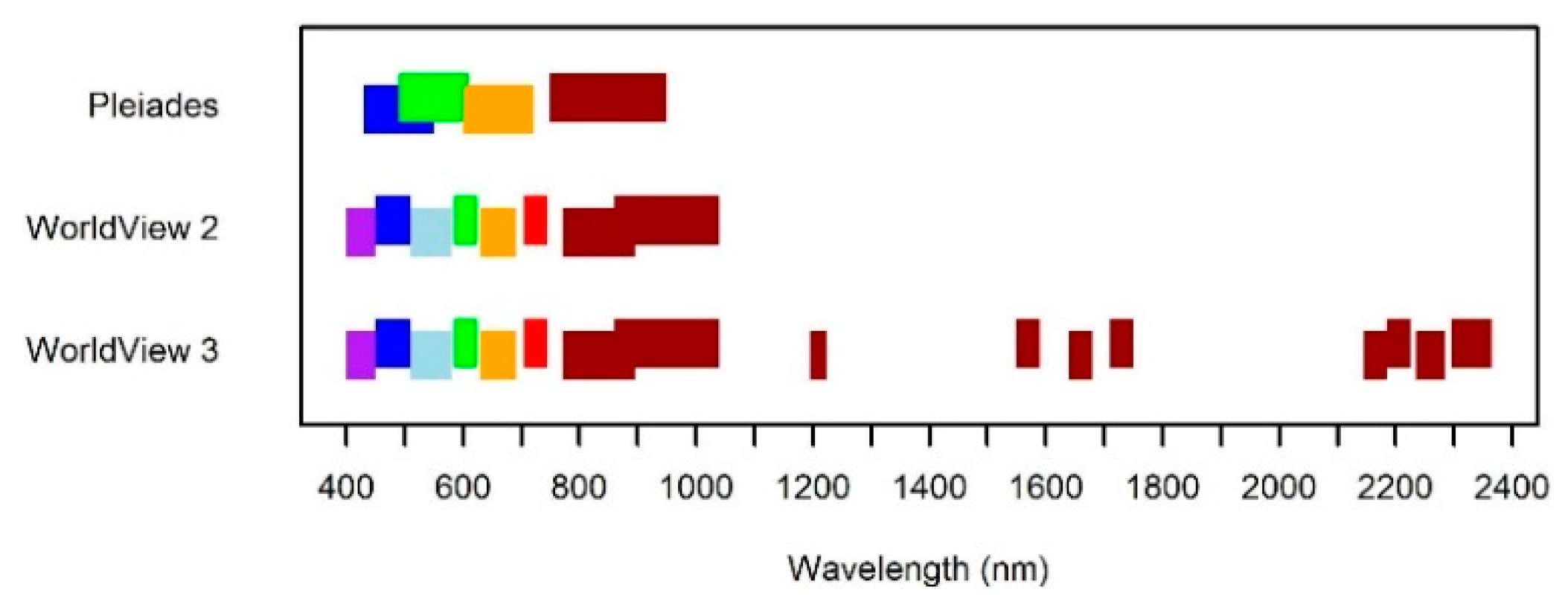
2. Materials and Methods
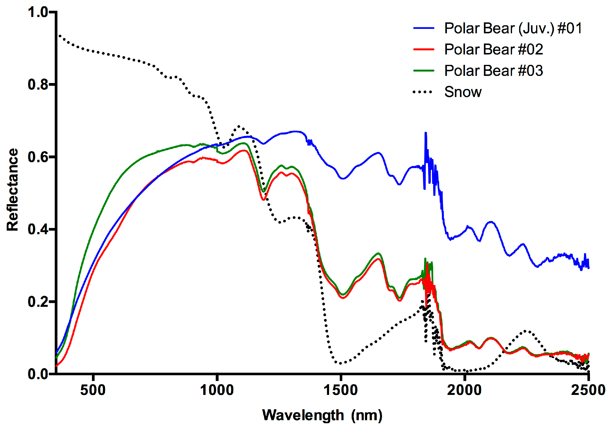
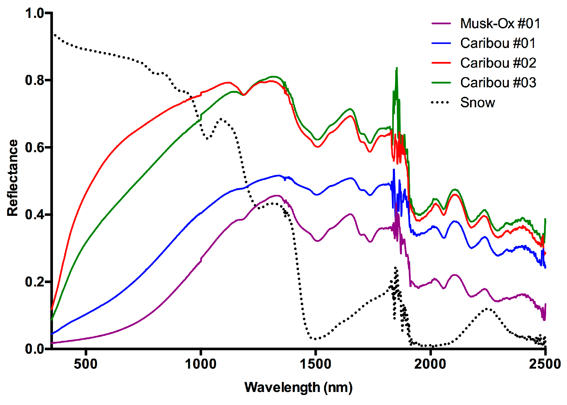
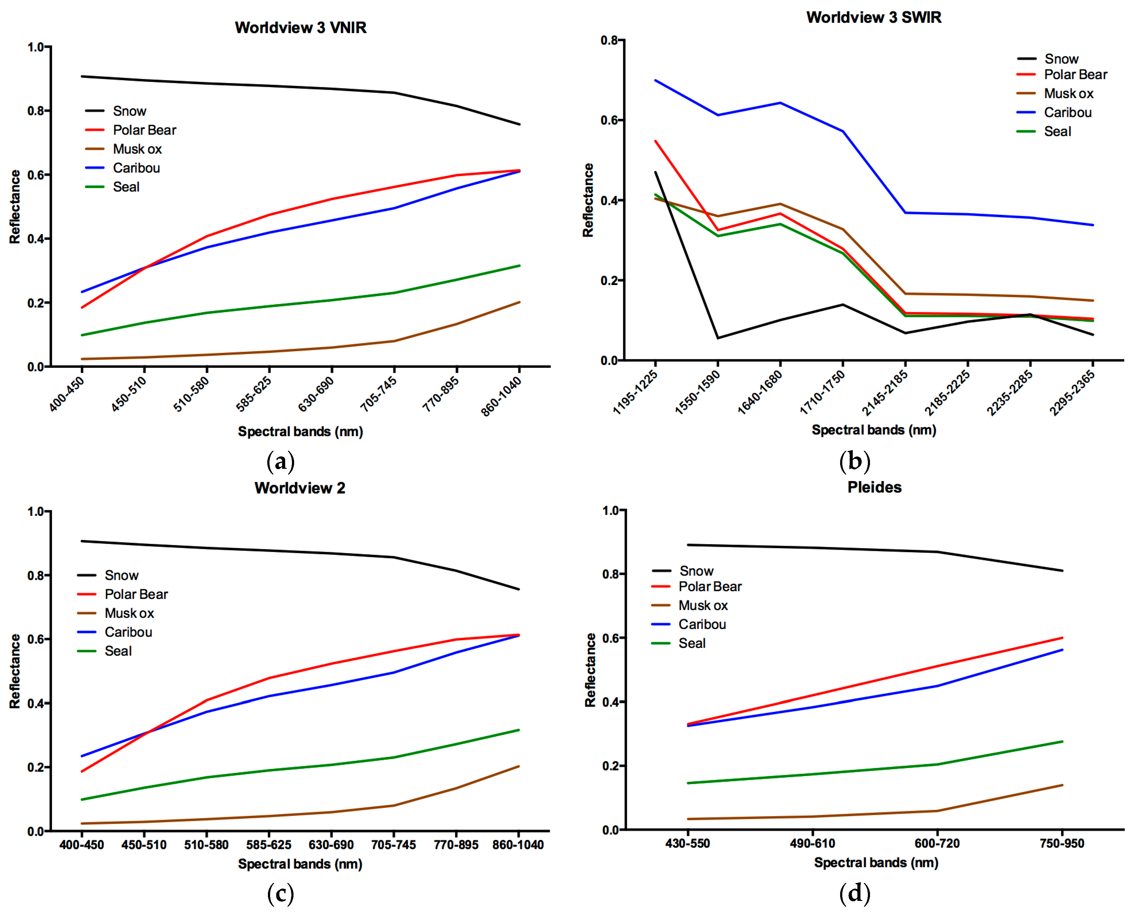
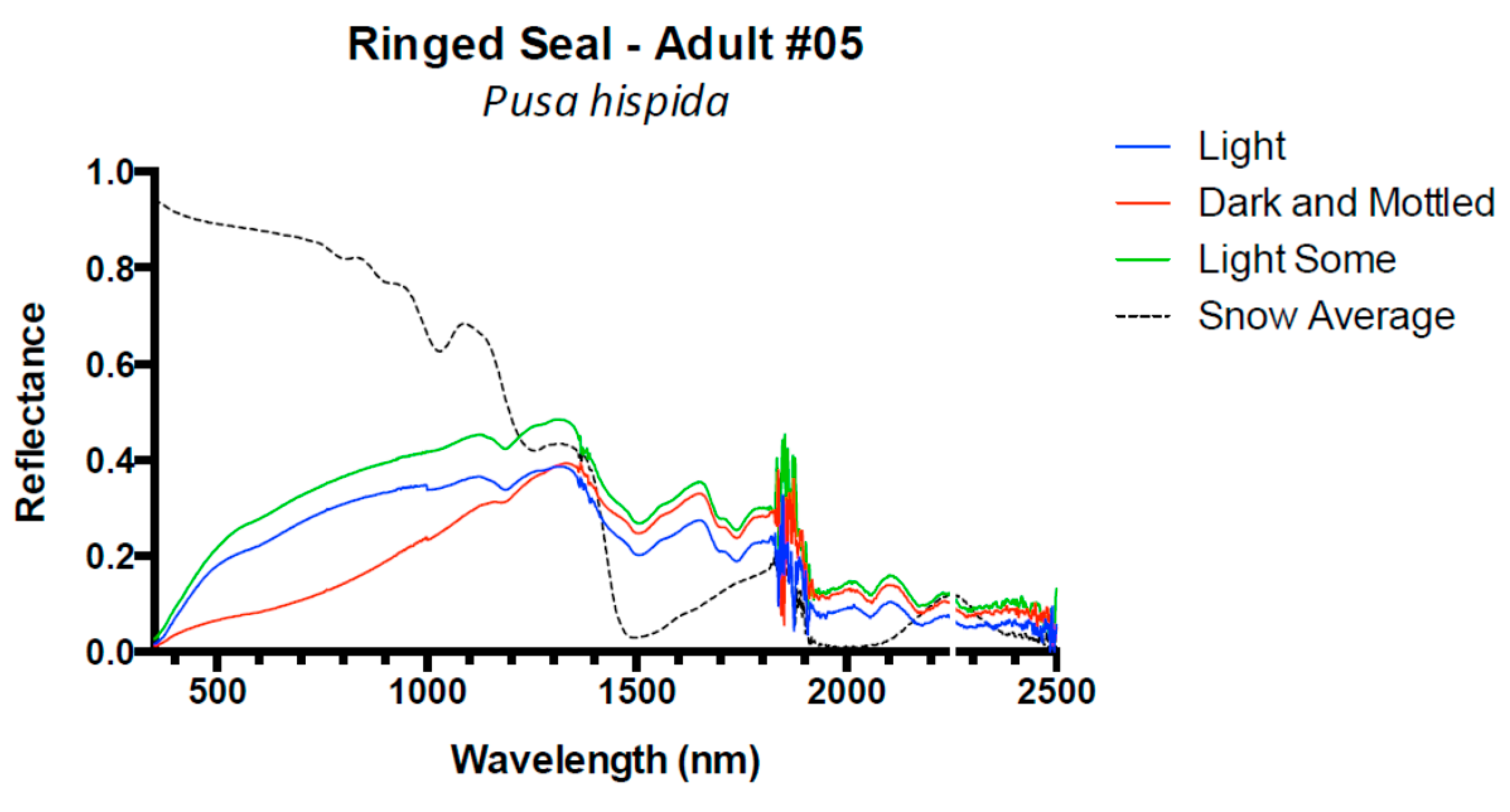
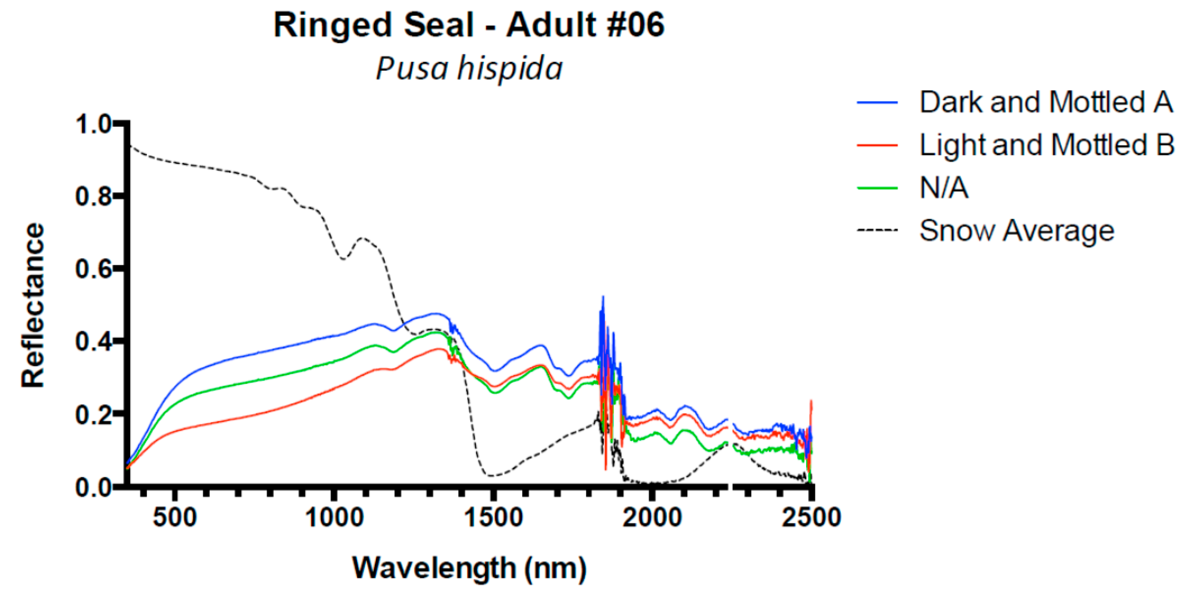
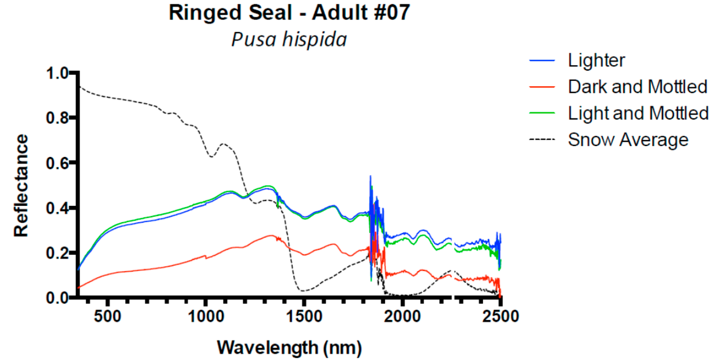
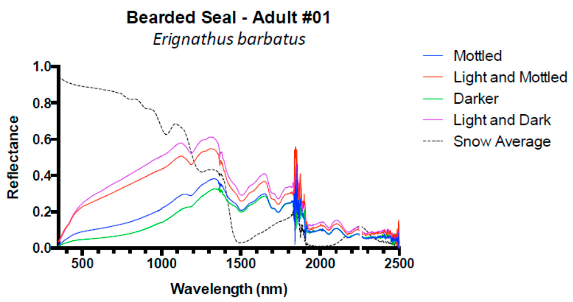
3. Results and Discussion
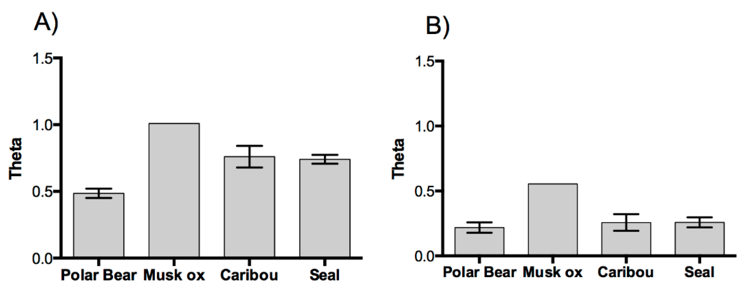
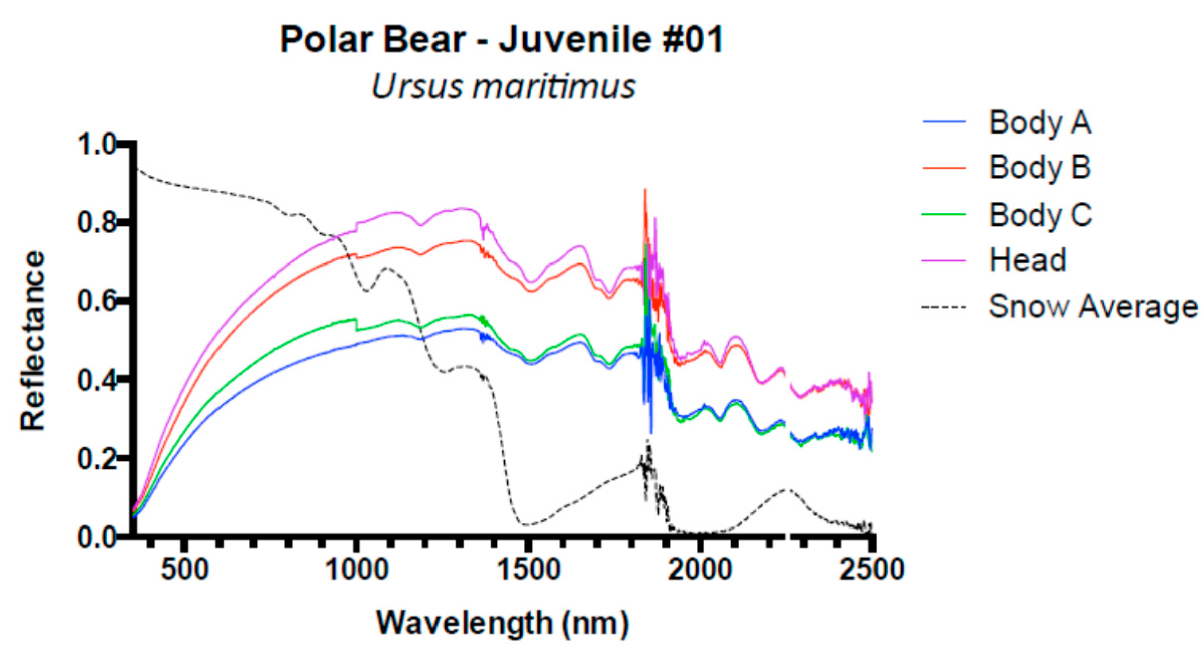
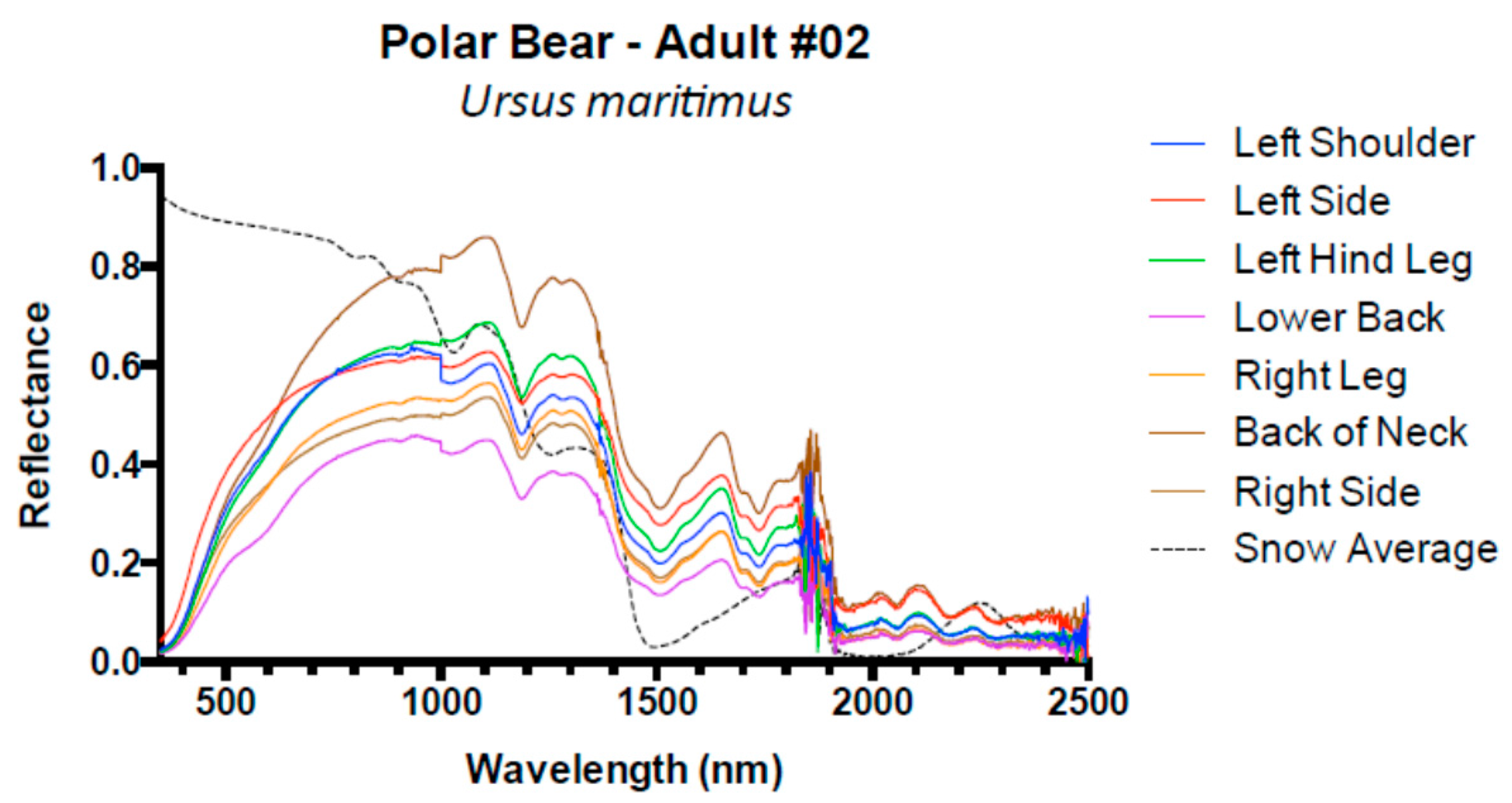
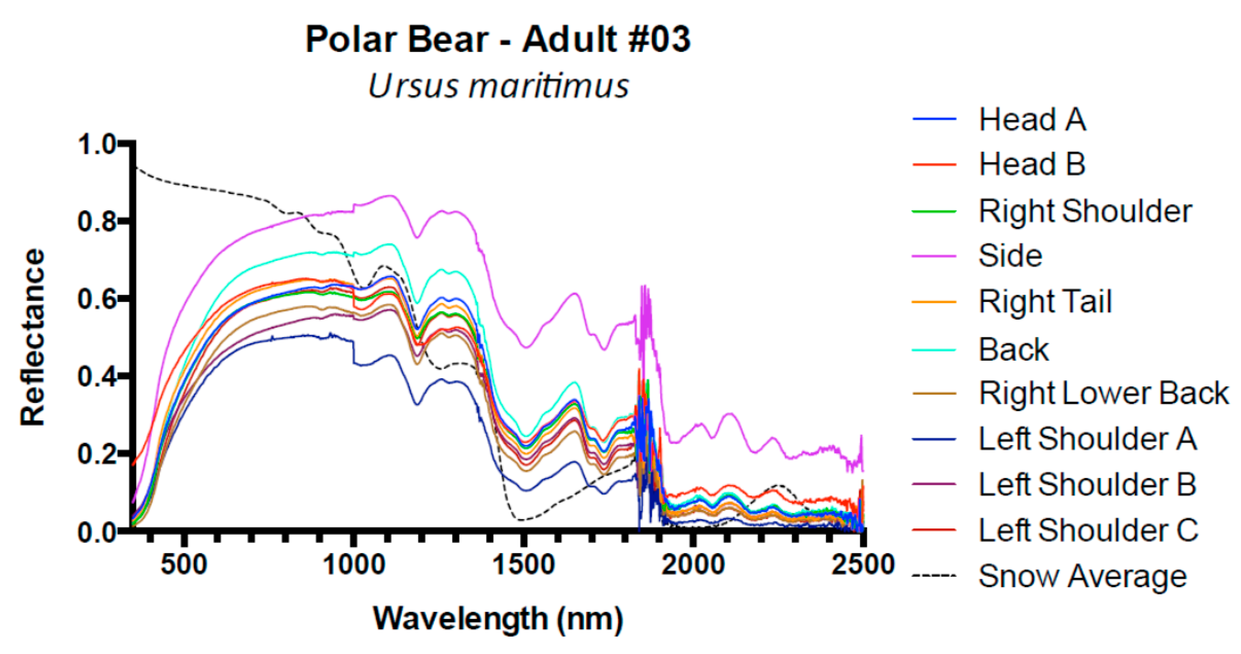
3.1. Results
3.2. Discussion
4. Conclusions
Acknowledgments
Author Contributions
Conflicts of Interest
Appendix A


References
- Comiso, J.C.; Parkinson, C.L.; Gersten, R.; Stock, L. Accelerated decline in the Arctic Sea ice cover. Geophys. Res. Lett. 2008, 35. [Google Scholar] [CrossRef]
- Regehr, E.V.; Lunn, N.J.; Amstrup, S.C.; Stirling, L. Effects of earlier sea ice breakup on survival and population size of polar bears in western Hudson bay. J. Wildl. Manag. 2007, 71, 2673–2683. [Google Scholar] [CrossRef]
- Stirling, I.; Parkinson, C.L. Possible effects of climate warming on selected populations of polar bears (Ursus maritimus) in the Canadian arctic. Arctic 2006, 59, 261–275. [Google Scholar] [CrossRef]
- Stirling, I.; Lunn, N.J.; Iacozza, J. Long-term trends in the population ecology of polar bears in western Hudson Bay in relation to climate change. Arctic 1999, 52, 294–306. [Google Scholar] [CrossRef]
- Stirling, I. Polar Bears: The Natural History of a Threatened Species; Fitzhenry and Whiteside: Markham, ON, Canada, 2011; p. 352. [Google Scholar]
- Aars, J.; Marques, T.A.; Buckland, S.T.; Andersen, M.; Belikov, S.; Boltunov, A.; Wiig, O. Estimating the Barents Sea polar bear subpopulation size. Mar. Mammal Sci. 2009, 25, 35–52. [Google Scholar] [CrossRef] [Green Version]
- Obbard, M.E.; Middel, K.R.; Stapleton, S.; Thibault, I.; Brodeur, V.; Jutras, C. Estimating Abundance of the Southern Hudson Bay Polar Bear Subpopulation using Aerial Surveys, 2011 and 2012; Ontario Ministry of Natural Resource, Science and Research Branch: Peterborough, ON, Canada, 2013. [Google Scholar]
- Stapleton, S.; Atkinson, S.; Hedman, D.; Garshelis, D. Revisiting western hudson bay: Using aerial surveys to update polar bear abundance in a sentinel population. Biol. Conserv. 2014, 170, 38–47. [Google Scholar] [CrossRef]
- Stapleton, S.; Peacock, E.; Garshelis, D.; Atkinson, S. Foxe Basin Polar Bear Aerial Survey, 2009 and 2010: Final Report; Government of Nunavut: Iqaluit, NU, Canada, 2012. [Google Scholar]
- Stapleton, S. Alternative Methods for Monitoring Polar Bears in the North American arctic. Ph.D. Thesis, University of Minnesota, Minneapolis, MN, USA, 2013. [Google Scholar]
- Stapleton, S.; LaRue, M.; Lecomte, N.; Atkinson, S.; Garshelis, D.; Porter, C.; Atwood, T. Polar bears from space: Assessing satellite imagery as a tool to track Arctic wildlife. PLoS ONE 2014, 9, e101513. [Google Scholar] [CrossRef] [PubMed]
- Kerbes, R.H.; Meeres, K.M.; Alisaukas, R.T.; Caswell, F.D.; Abraham, K.F.; Ross, R.K. Surveys of Nesting Mid-Continent Lesser Snow Geese and Ross’s Geese in Eastern and Central Arctic Canada, 1997–1998; Technical Report Series No. 447; Canadian Wildlife Service, Prarie and Northern Region: Saskatoon, Saskatchewan, 2006. [Google Scholar]
- Conn, P.B.; Hoef, J.M.V.; McClintock, B.T.; Moreland, E.E.; London, J.M.; Cameron, M.F.; Dahle, S.P.; Boveng, P.L. Estimating multispecies abundance using automated detection systems: Ice-associated seals in the Bering Sea. Methods Ecol. Evolut. 2014, 5, 1280–1293. [Google Scholar] [CrossRef]
- Guinet, C.; Jouventin, P.; Malacamp, J. Satellite remote sensing in monitoring change of seabirds: Use of Spot Image in king penguin population increase at the Ile aux Cochons, Crozet Archipelago. Polar Biol. 1995, 15, 511–515. [Google Scholar] [CrossRef]
- Barber-Meyer, S.M.; Kooyman, G.L.; Ponganis, P.J. Estimating the relative abundance of emperor penguins at inaccessible colonies using satellite imagery. Polar Biol. 2007, 30, 1565–1570. [Google Scholar] [CrossRef]
- Fretwell, P.; LaRue, M.; Morin, P.; Kooyman, G.L.; Wienecky, B.; Ratcliffe, N.; Fox, A.; Fleming, A.; Porter, C.; Trathan, P. An emperor penguin population estimate: The first global, synoptic survey of a species from space. PLoS ONE 2012, 7, e33751. [Google Scholar] [CrossRef]
- LaRue, M.; Rotella, J.; Garrott, R.; Siniff, D.; Ainley, D.; Stauffer, G.; Porter, C.; Morin, P. Satellite imagery can be used to detect variation in abundance of Weddell seals (Leptonychotes weddellii) in Erebus Bay, Antarctica. Polar Biol. 2011, 34, 1727–1737. [Google Scholar] [CrossRef]
- Platonov, N.G.; Mordvintsev, I.N.; Rozhnov, V.V. The possibility of using high resolution satellite imagery for detection of marine mammals. Biol. Bull. 2013, 40, 197–205. [Google Scholar] [CrossRef]
- Lavigne, D.M.; Øritsland, N.A. Black polar bears. Nature 1974, 251, 218–219. [Google Scholar] [CrossRef]
- Lavigne, D.M.; Øritsland, N.A. Ultraviolet photography: A new application for remote sensing of mammals. Can. J. Zool. 1974, 52, 939–941. [Google Scholar] [CrossRef] [PubMed]
- Øritsland, N.A.; Lavigne, D.M. Radiative surface temperatures of exercising polar bears. Comp. Biochem. Physiol. A Physiol. 1976, 53, 327–330. [Google Scholar] [CrossRef]
- Grojean, R.E.; Sousa, J.A.; Henry, M.C. Utilization of solar radiation by polar animals: An optical model for pelts. Appl. Opt. 1980, 19, 339–346. [Google Scholar] [CrossRef] [PubMed]
- Burn, D.M.; Udevitz, M.S.; Speckman, S.G.; Benter, R.B. An improved procedure for detection and enumeration of walrus signatures in airborne thermal imagery. Int. J. Appl. Earth Obs. Geoinf. 2009, 11, 324–333. [Google Scholar] [CrossRef]
- Brooks, J.W. Infrared scanning for polar bear. In Proceedings of the International Conference on Bear Research and Management, Calgary, AB, Canada, 6–9 November 1972; pp. 138–141.
- Amstrup, S.C. Polar bear, Ursus maritimus. In Wild Mammals of North America: Biology, Management, and Conservation; Feldhamer, G.A., Thompson, B.C., Chapman, J.A., Eds.; Johns Hopkins University Press: Baltimore, MD, USA, 2003; pp. 587–610. [Google Scholar]
- Watts, P.D. Ecological Energetics of Denning Polar Bears and Related Species. Ph.D. Thesis, University of Oslo, Oslo, Norway, 1983. [Google Scholar]
- Amstrup, S.C.; York, G.; McDonald, T.L.; Nielson, R.; Simac, K. Detecting denning polar bears with forward-looking infrared (FLIR) imagery. Bioscience 2004, 54, 337–344. [Google Scholar] [CrossRef]
- Kimes, D.S.; Kirchner, J.A.; Newcomb, W.W. Spectral radiance errors in remote-sensing ground studies due to nearby objects. Appl. Opt. 1983, 22, 8–10. [Google Scholar] [CrossRef] [PubMed]
- Price, J.C. How unique are spectral signatures. Remote Sens. Environ. 1994, 49, 181–186. [Google Scholar] [CrossRef]
- Satellite Imaging Corporation. Available online: http://www.satimagingcorp.com/satellite-sensors/ (accessed on 16 March 2016).
- Eastman Kodak Company. KODAK Double-X Aerographic Film 2405; Eastman Kodak Company: Rochester, NY, USA, 2005. [Google Scholar]
- Downing, S.C. Color changes in mammal skins during preparation. J. Mammol. 1945, 26, 128–132. [Google Scholar] [CrossRef]
- Davis, A.K.; Woodall, N.; Moskowitz, J.P.; Castleberry, N.; Freeman, B.J. Temporal change in fur color in museum specimens of mammals: Reddish-brown species get redder with storage time. Int. J. Zool. 2013, 2013, 876347. [Google Scholar] [CrossRef]
- DeMaster, D.P.; Stirling, I. Ursus maritimus. Mamm. Species 1981, 145, 1–7. [Google Scholar] [CrossRef]
- Gerland, S.; Winther, J.G.; Orbaek, J.B.; Ivanov, B.V. Physical properties, spectral reflectance and thickness development of first year fast ice in Kongsfjorden, Svalbard. Polar Res. 1999, 18, 275–282. [Google Scholar] [CrossRef]


| Time (Local) | Air Temp.* (°C) | Dew Point * (°C) | Relative Humidity * (%) | Visibility * (Km) | Solar Zenith † (°) |
|---|---|---|---|---|---|
| 13:22 | −5.4 | −17.8 | 37 | 24.1 | 52.5 |
| 14:22 | −4.1 | −18.1 | 33 | 24.1 | 56.6 |
| Mammal Species | Pelt # | Age | # of Samples |
|---|---|---|---|
| Ringed Seal, Pusa hispida | 1 | Adult | 3 |
| 2 | Adult | 2 | |
| 3 | Juvenile | 2 | |
| 4 | Adult | 3 | |
| 5 | Adult | 3 | |
| 6 | Adult | 3 | |
| 7 | Adult | 3 | |
| 8 | Adult | 3 | |
| Harp Seal, Pagophilus groenlandicus | 1 | Adult | 6 |
| Bearded Seal, Erignatus barbatus | 1 | Adult | 4 |
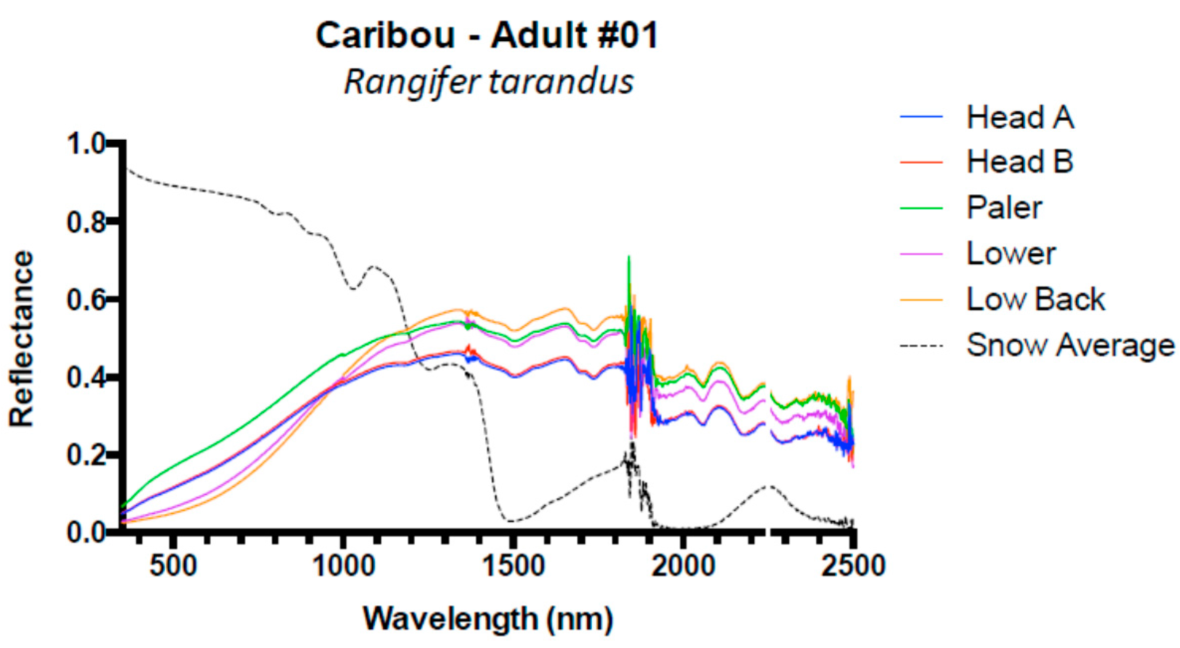
| Caribou Rangifer tarandus | 1 | Adult | 5 |
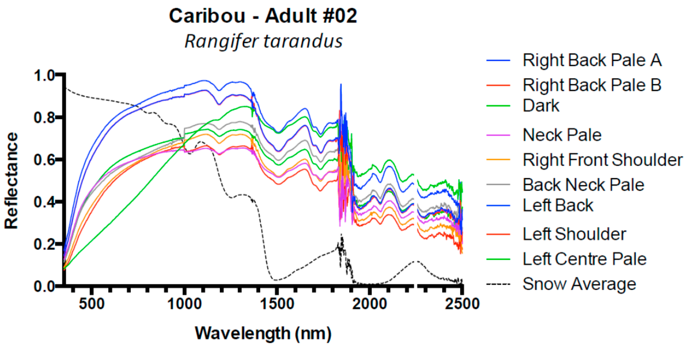
| 2 | Adult | 9 | |
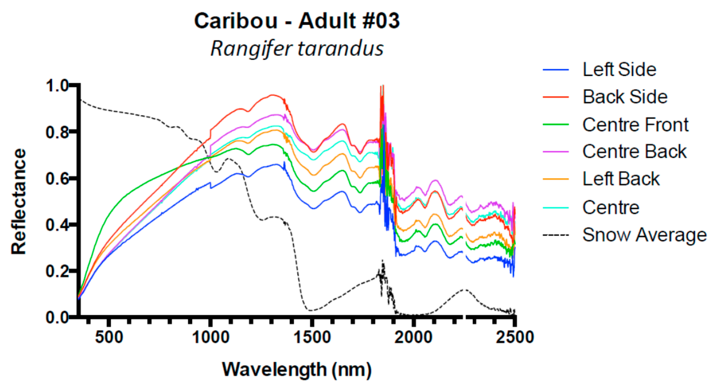
| 3 | Adult | 6 | |
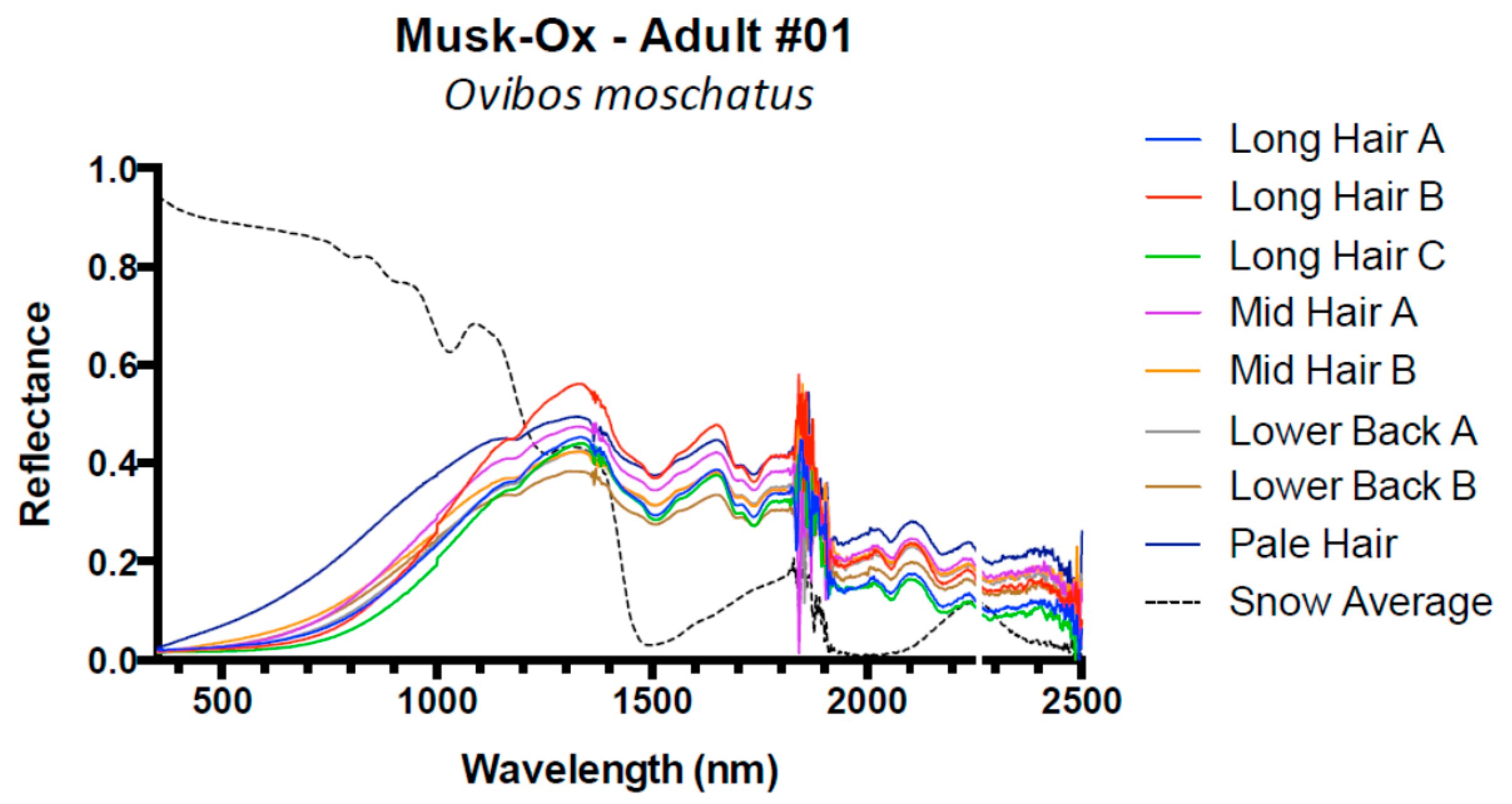
| Musk-Ox, Ovibos moschatus | 1 | Adult | 8 |
| Polar Bear, Ursus maritimus | 1 | Juvenile | 4 |
| 2 | Adult | 7 | |
| 3 | Adult | 10 |
| Slope of Average Spectra (% Reflectance/nm) | |||||
|---|---|---|---|---|---|
| Sample Material | n | UVA (350–400 nm) | VIS (400–770 nm) | NIR (770–1000 nm) | SWIR (1000–2450 nm) |
| Snow | 10 | −0.06 (±0.01) | −0.02 (±0.00) | −0.07 (±0.00) | −0.04 (±0.00) |
| Polar bear (Adult) | 2 | 0.13 (±0.03) | 0.15 (±0.01) | 0.01 (±0.01) | −0.04 (±0.01) |
| Polar bear (Juv.) | 1 | 0.15 | 0.12 | 0.04 | −0.02 |
| Caribou | 3 | 0.16 (±0.1) | 0.09 (±0.01) | 0.06 (±0.01) | −0.02 (±0.01) |
| Muskox | 1 | 0.01 | 0.02 | 0.07 | −0.01 |
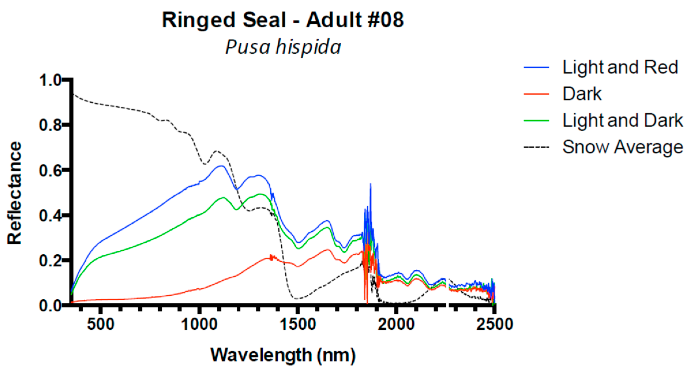
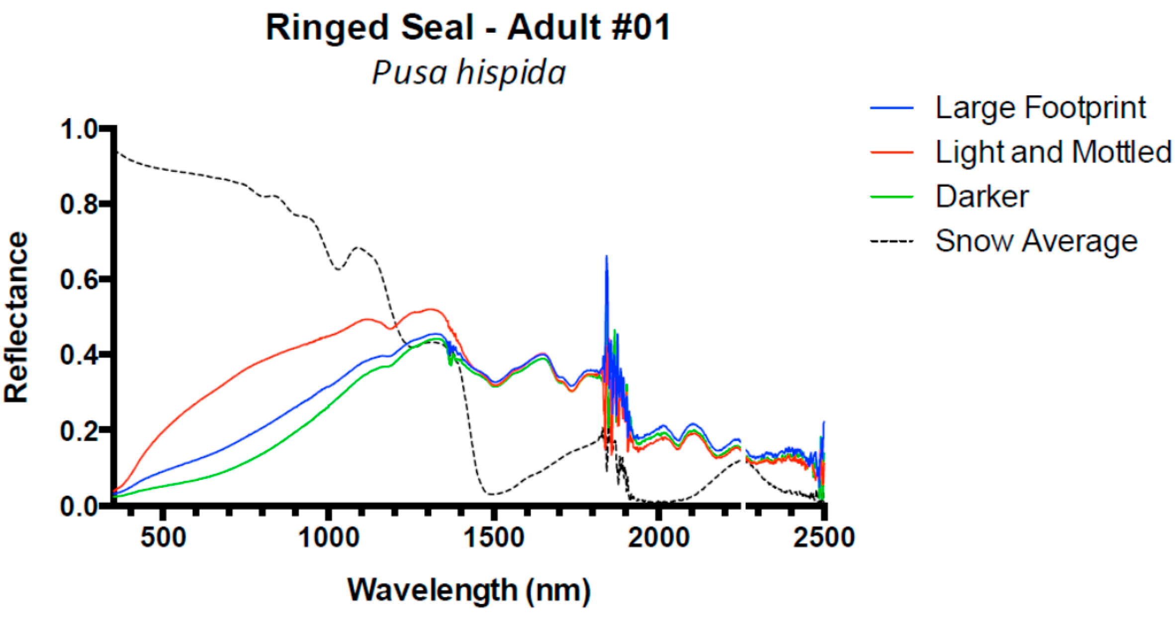
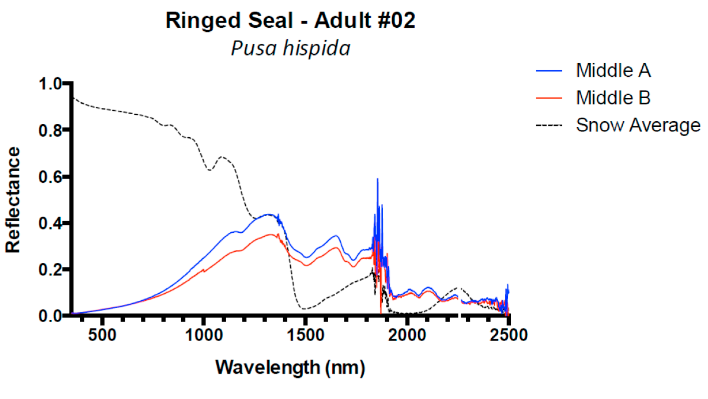
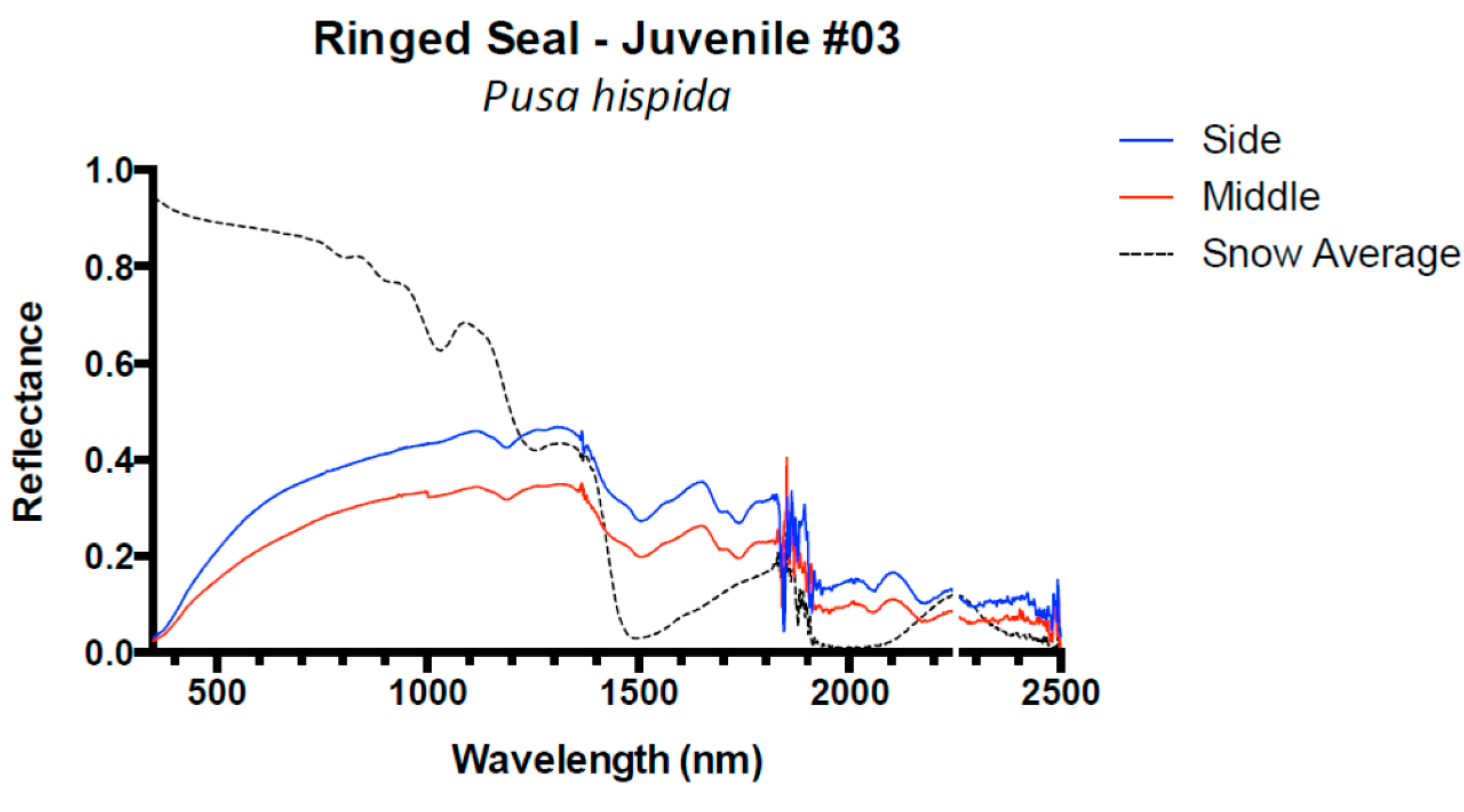
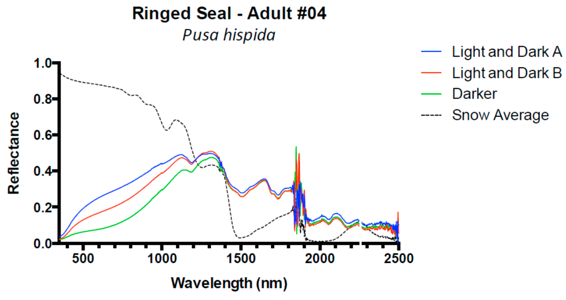
| Ringed Seal | 8 | 0.08 (±0.02) | 0.05 (±0.02) | 0.04 (±0.01) | −0.02 (±0.00) |
| Bearded seal | 1 | 0.10 | 0.04 | 0.04 | −0.02 |
| Harp seal | 1 | 0.04 | 0.06 | 0.07 | −0.02 |
| Curvature of Spectrum (% Reflectance/nm) | ||||||||||||
|---|---|---|---|---|---|---|---|---|---|---|---|---|
| Sample Material | UVA (350–400 nm) | VIS (400–700 nm) | NIR (700–1000 nm) | SWIR(1000–2450 nm) | ||||||||
| Average Deviation % | Largest Deviation | Average Deviation % | Largest Deviation | Average Deviation % | Largest Deviation | Average Deviation % | Largest Deviation | |||||
| % | nm | % | Nm | % | nm | % | Nm | |||||
| Snow | −0.1 | −0.1 | 380 | −0.3 | 0.0 | 684 | 3.3 | 6.0 | 950 | −14.0 | −42.0 | 1484 |
| Polar Bear #1 (Juvenile) | −0.8 | −1.4 | 380 | 7.9 | 11.6 | 518 | 1.3 | 2.1 | 865 | 3.7 | 12.7 | 1654 |
| Polar Bear #2 | −0.5 | −0.9 | 377 | 3.4 | 5.3 | 550 | 1.3 | 1.3 | 855 | −5.3 | −18.9 | 1502 |
| Polar Bear #3 | −0.6 | −1.0 | 387 | 3.9 | 6.8 | 518 | 3.4 | 3.4 | 947 | −6.5 | −20.5 | 1503 |
| Caribou #1 | −0.1 | −0.1 | 374 | −0.5 | −1.0 | 596 | 0.1 | 0.7 | 942 | 7.2 | 15.9 | 1655 |
| Caribou #2 | −0.5 | −0.8 | 376 | 5.4 | 8.0 | 516 | 0.8 | 1.2 | 857 | 3.2 | 13.6 | 1331 |
| Caribou #3 | −0.2 | −0.3 | 377 | 2.5 | 4.0 | 503 | 0.6 | 1.0 | 890 | 6.7 | 20.2 | 1332 |
| Musk-Ox | −0.0 | −0.1 | 364 | −0.6 | −1.0 | 579 | −1.2 | −1.9 | 823 | 9.3 | 22.5 | 1338 |
| Ringed Seal #1 | −0.2 | −0.4 | 380 | 0.7 | 1.3 | 487 | −0.1 | −0.3 | 941 | 6.6 | 18.3 | 1329 |
| Ringed Seal # 2 | −0.1 | −0.2 | 372 | −0.4 | −0.6 | 585 | −1.3 | −2.1 | 846 | 7.3 | 21.0 | 1335 |
| Ringed Seal #3 (Juvenile) | −0.4 | −0.7 | 380 | 2.4 | 3.5 | 566 | 0.7 | 1.0 | 853 | 0.0 | 9.0–9.0 | 1330 1935 |
| Ringed Seal # 4 | −0.3 | −0.5 | 375 | 1.5 | 2.4 | 502 | −1.0 | −1.7 | 834 | 3.0 | 17.8 | 1324 |
| Ringed Seal # 5 | −0.3 | −0.6 | 371 | 1.8 | 3.2 | 518 | 0.3 | 0.6 | 934 | −0.5 | 10.7 | 1331 |
| Ringed Seal # 6 | −0.2 | −0.3 | 381 | 3.1 | 5.0 | 517 | −0.2 | −0.4 | 814 | 3.7 | 13.5 | 1333 |
| Ringed Seal # 7 | 0.2 | 0.3 | 367 | 2.4 | 3.9 | 517 | −0.4 | −0.8 | 817 | 5.7 | 12.7 | 1329 |
| Ringed Seal # 8 | 0.2 | 0.3 | 389 | 1.4 | 2.6 | 488 | 0.0 | 0.7 | 946 | 2.7 | 14.3 | 1328 |
| Bearded Seal #1 | −0.0 | −0.2 | 361 | 1.7 | 3.0 | 489 | −0.3 | −0.5 | 830 | 4.8 | 20.2 | 1329 |
| Harp Seal #1 | −0.2 | −0.3 | 376 | 0.5 | 0.9 | 518 | −0.4 | −0.7 | 814 | 4.5 | 22.5 | 1319 |
© 2016 by the authors; licensee MDPI, Basel, Switzerland. This article is an open access article distributed under the terms and conditions of the Creative Commons by Attribution (CC-BY) license (http://creativecommons.org/licenses/by/4.0/).
Share and Cite
Leblanc, G.; Francis, C.M.; Soffer, R.; Kalacska, M.; De Gea, J. Spectral Reflectance of Polar Bear and Other Large Arctic Mammal Pelts; Potential Applications to Remote Sensing Surveys. Remote Sens. 2016, 8, 273. https://doi.org/10.3390/rs8040273
Leblanc G, Francis CM, Soffer R, Kalacska M, De Gea J. Spectral Reflectance of Polar Bear and Other Large Arctic Mammal Pelts; Potential Applications to Remote Sensing Surveys. Remote Sensing. 2016; 8(4):273. https://doi.org/10.3390/rs8040273
Chicago/Turabian StyleLeblanc, George, Charles M. Francis, Raymond Soffer, Margaret Kalacska, and Julie De Gea. 2016. "Spectral Reflectance of Polar Bear and Other Large Arctic Mammal Pelts; Potential Applications to Remote Sensing Surveys" Remote Sensing 8, no. 4: 273. https://doi.org/10.3390/rs8040273