Article

Bayesian Analysis of Uncertainty in the GlobCover 2009 Land Cover Product at Climate Model Grid Scale

1
National Centre for Earth Observation, Department of Meteorology, University of Reading, Reading, Berkshire RG6 6AH, UK
2
School of Mathematics and Statistics, University of Western Australia, Crawley WA 6009, Australia
*
Author to whom correspondence should be addressed.
Remote Sens. 2016, 8(4), 314; https://doi.org/10.3390/rs8040314
Submission received: 26 November 2015 / Revised: 15 March 2016 / Accepted: 22 March 2016 / Published: 8 April 2016
(This article belongs to the Special Issue Validation and Inter-Comparison of Land Cover and Land Use Data)

Abstract

:
Land cover data derived from satellites are commonly used to prescribe inputs to models of the land surface. Since such data inevitably contains errors, quantifying how uncertainties in the data affect a model’s output is important. To do so, a spatial distribution of possible land cover values is required to propagate through the model’s simulation. However, at large scales, such as those required for climate models, such spatial modelling can be difficult. Also, computer models often require land cover proportions at sites larger than the original map scale as inputs, and it is the uncertainty in these proportions that this article discusses. This paper describes a Monte Carlo sampling scheme that generates realisations of land cover proportions from the posterior distribution as implied by a Bayesian analysis that combines spatial information in the land cover map and its associated confusion matrix. The technique is computationally simple and has been applied previously to the Land Cover Map 2000 for the region of England and Wales. This article demonstrates the ability of the technique to scale up to large (global) satellite derived land cover maps and reports its application to the GlobCover 2009 data product. The results show that, in general, the GlobCover data possesses only small biases, with the largest belonging to non–vegetated surfaces. In vegetated surfaces, the most prominent area of uncertainty is Southern Africa, which represents a complex heterogeneous landscape. It is also clear from this study that greater resources need to be devoted to the construction of comprehensive confusion matrices.

Graphical Abstract

1. Introduction

Since the advent of global imaging satellites such as AVHRR, the production of data on land cover at global scales has been the focus of much effort internationally. Over the last decade several such products have been released, including the MODIS land cover product suite [1,2], the Global Land Cover 2000 product (GLC2000) [3], and the GlobCover products [4,5]. An important use for these data is providing the spatial distribution of variables, such as Plant Functional Type (PFT), for Earth System Models of varying degrees of complexity. For example, [6] used the AVHRR land cover map developed by [7] to prescribe dominant cover in the US National Centre for Atmospheric Research (NCAR) land model, and [8] parameterised a simple ecosystem model with MODIS land cover data to estimate the regional carbon budgets in the Mid-West US. Some Dynamic Global Vegetation Models (DGVMs) are able to ingest land cover data to initialise a dynamic run (i.e., where the DGVM predicts competition between PFTs over time) or simply to prescribe static PFTs for the calculation of contemporary carbon budgets. Examples of the use of satellite-derived land cover in DGVMs are given by [9,10]. Some models of this type are designed to be used as the lower boundary for climate models, and any errors in the model outputs have the potential to feed into climate simulations. Satellite derived land cover data are also used in atmospheric transport model inversion-based estimates of land–atmosphere fluxes of various chemical species: [11] use the continuous vegetation fields produced by [12,13] to analyse the results of global inversions of CO 2 and O 2 data; [14] used MODIS land cover data to assign SiB3 biome types for estimating high resolution carbon fluxes using atmospheric inversion; [15] used the GLC2000 product to delineate tropical forest for N 2 O emissions inventories.
Since remotely sensed land cover data inevitably contain mis-classifications, various methods have been proposed to characterise the uncertainty associated with land cover maps constructed by the the remote sensing community. Generally, quantifying uncertainty falls into one of three categories: comparison against ground data, analysis of classification statistics (e.g., measures of separation in spectral space), or comparisons between different land cover products. Comparison against ground truth provides, in principle, the fullest description of the errors in land cover data. The ideal scenario is that a very large number of sites are visited and the land cover present at each is compared with that in the remote sensing land cover map. This information is typically encoded in a confusion matrix, which provides the user of the data with an easily interpretable overview of which classes are most likely to be incorrectly classified (and as what classes) as well as an overall measure of mis-classification in the product. Further details are provided in Section 2.2 and a comprehensive description of the construction of such matrices and issues surrounding them is given by [16]. In practice, it is often prohibitively time consuming or too expensive to obtain enough samples. Furthermore, correctly representing the spatial scale of the satellite data from the ground samples is problematic. Consequently, it is becoming more common to construct confusion matrices against higher resolution satellite data that has been interpreted manually. Such a matrix is used in this study and is described in greater detail in the methods section. Classification statistics, such as entropy measures described by [17], are not considered in this paper but may provide useful additional information in further studies. In essence, these methods assume that the more homogeneous the maximum likelihood of a given class is (i.e., the lower its entropy) the more accurate the classification. If this assumption holds, then the information could, in principle, be used directly in the statistical model presented here. However, because the most readily available information on classification accuracy is typically in the form of a confusion matrix, this is the focus of the current study. Comparisons between land cover products, such as that presented by [18], are useful for identifying problematic regions or classes but cannot provide a probabilistic measure of uncertainty and are hence not considered here.
Despite the efforts taken to describe the uncertainty in satellite derived land cover data, little has been done to assess the direct impact of these uncertainties on the predictions of large scale land surface models, such as DGVMs. Quaife et al. [19] used various 1 k m land cover data to prescribe PFT distribution for the Sheffield Dynamic Vegetation Model [20] and compared the predicted carbon balance to that predicted by the same model using a nominally accurate land cover map of the UK. The results showed large discrepancies in the net carbon balance of the UK, depending on which land cover product was used. Poulter et al. [21] define an index of dissimilarity between several satellite land cover products to diagnose likely causes of uncertainties in modelled variables on global scales, but the uncertainties are not propagated through a model. Neither of these studies directly quantifies the impact of uncertainty in an individual land cover product on model outputs. Rather, they infer uncertainty by comparison with other land cover data sets. While these studies are undoubtedly valuable, there is an obvious need for techniques that connect the information on land cover uncertainty from the remote sensing community with the needs of the modelling community.
It is important to acknowledge that the confusion matrix does not encompass all of the errors associated with land cover data that might affect a land surface model. Perhaps the largest of these is the translation between land cover classes represented in the remote sensing product and the plant functional types required by a model. In some instances the translation is unambiguous; for example, if a land cover classification reports 100% presence of deciduous broadleaved trees, it is clear as to which PFT this should be assigned. However, this is rarely the case. Often classification schemes report mixed land cover classes with unspecified proportions or proportions within given ranges. This is true of many of classes in the GlobCover maps, which are the focus of this paper. Typically, the translation between land cover classification is done using subjective methods and hence contain potentially significant errors. This is explored in detail in [21].
This papers focuses on errors in the classification alone. The motivation behind this is to illustrate a technique for producing estimates of uncertainty in satellite derived land cover maps on large scales, which can subsequently be propagated through a model so as to understand the sensitivity of its prognostics variables to likely classification errors. Future work will extend this to incorporate errors in land cover to PFT translation.
Often the remotely sensed pixels are aggregated to a site (in the order of 1 ) for the user to incorporate into their model and represented as the proportion of different cover types within each grid–cell. This article provides a Bayesian hierarchical model from which we are able to simulate the proportions of true land cover types in each site, across the entire region, thereby providing spatially varying posterior standard deviations to quantify uncertainty. Since the remotely sensed pixels are potentially mis-classified, we treat the true land cover proportions in each site as latent variables and model them by combining a spatial prior distribution constructed from the remotely sensed recordings with data in the confusion matrix. The method not only models the spatial variation in the true land cover values, but also the spatial variation in the errors of the remotely sensed data through the confusion matrix. The spatial prior is constructed for the site-specific probabilities of true land classes and is an approximation to a Markov random field prior. The model for the region wide confusion matrix is similar to that of [22,23], but rather than modelling the probabilities of the true classes, conditioned on the remotely sensed map, we model the probabilities of the remote sensed map classes, conditioned on the true classes, and we allow these map error probabilities to vary spatially.
One advantage of our method is in allowing for a Monte Carlo simulation scheme that generates from the posterior distribution of true land cover proportions that easily computes when applied to large scale problems. The output of the simulation scheme can then be used as inputs to any model that requires land cover data as an input, and can consequently estimate likely errors in model outputs due to uncertainties in land cover information. The statistical method is described in detail in [
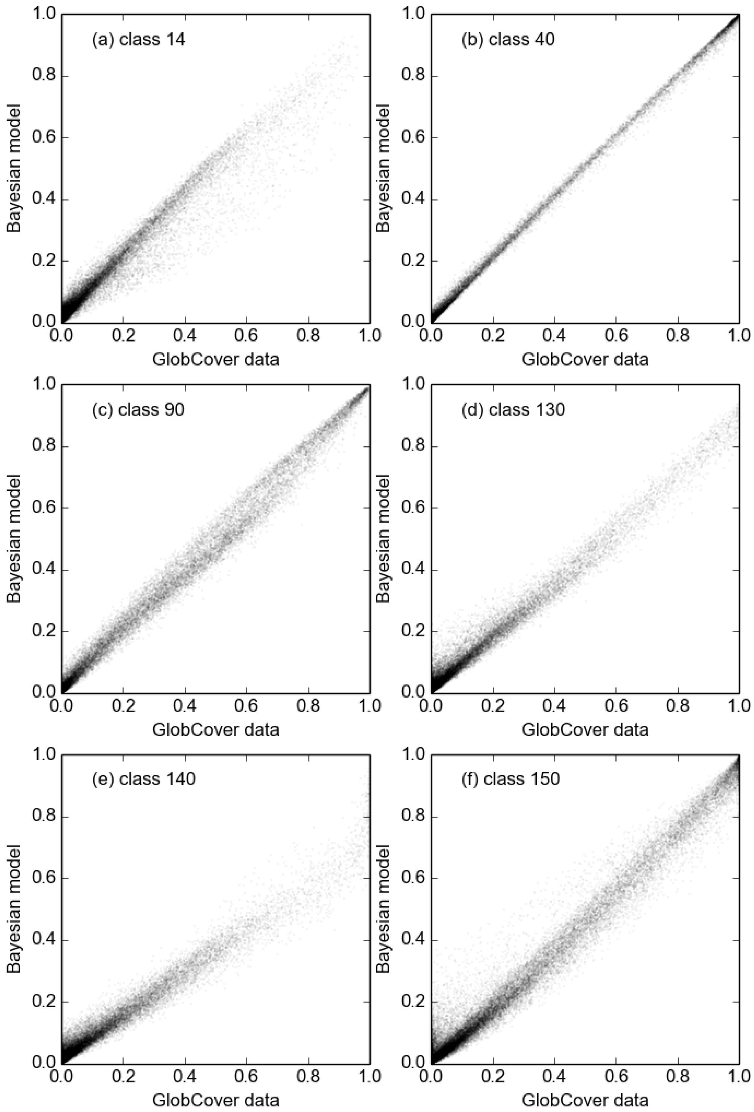
24], where it is demonstrated on a relatively small number of pixels representing a handful of PFTs. In this article, the method is applied to the GlobCover 2009 data set at the global scale, using the full range of land cover classes. This highlights the utility of the method for working with global land surface and climate models. The results show the spatial distribution of errors in the GlobCover data and the performance of a subset of the classes is explored.

2. Data

2.1. GlobCover 2009

GlobCover is a European Space Agency initiative to produce global land cover maps from MERIS 300 m data. Currently, it has produced two such maps, covering the periods December 2004–June 2006 and January–December 2009. The GlobCover product represents 22 land cover classes based on the UN Land Cover Classification System (LCCS), which are given in Table 1. Around 20 terabytes of MERIS reflectance data were processed using a combination of supervised and unsupervised classification to produce the 2009 product. For the purpose of this study, the GlobCover 2009 product was resampled to a 1 2 grid, calculating the proportion of each land cover type in each grid–cell. As the nominal projection of the data is on a Plate–Carrée latitude–longitude grid, no geographic re-projection was required.
For the purpose of the analysis presented here, a land mask has been applied to the data to exclude ocean areas. Consequently, the results for class 210 correspond only to coastal and inland water bodies.

2.2. Confusion Matrix

A confusion matrix represents a tally of comparisons of a land cover map against some form of validation. Numbers on the leading diagonal correspond to samples from the land cover map that are in agreement with the validation data and off-diagonal elements show the number of samples that were incorrectly classified as each of the other land cover types. Consequently, this information explicitly accounts for both errors of omission and commission. Sums of rows and columns provide marginal values for each class, which, when compared to the leading diagonal, are often referred to as the “user’s” (i.e., commission) and “producer’s” (i.e., omission) accuracies. As well as providing a quantitative means of describing errors in classification data, confusion matrices are also used in methods to improve classifications [25].
The GlobCover 2009 product contains two such matrices constructed against a comprehensive set of high resolution image data, which have been interpreted by local experts [4]. In this study, the matrix built using “certain” and “heterogeneous” validation points (shown in Table 2) has been used for two reasons. First, it reports a higher degree of uncertainty in the land cover (overall accuracy of 58 . 0 % ), and consequently, the results of the analysis presented here will represent an upper bound on the uncertainty of the product. Second, for practical reasons it is not possible to use the matrix generated from the “certain” and “homogeneous” validation data, as not all land cover classes have been sampled, and hence it is not possible to apply the proposed method.
The distinction between the heterogeneous and homogeneous confusion matrices is the nature of land cover at the points in the data set used to construct them. The homogeneous matrix (i.e., the one not used in this study) only uses data from pixels where the land cover belongs to a singular class in the high resolution validation data set. The heterogeneous matrix also uses these data points, but additionally includes data where the land cover is mixed. Consequently, it contains a larger number of samples (2190 vs. 1408).
Table 1 contains additional information derived from the confusion matrix: the total number of samples in the reference data set, and the producer’s and user’s accuracies. The producer’s accuracy is a measure of how likely an area represented by a pixel on the ground is correctly classified, and the user’s accuracy is a measure of how likely a pixel classified as a given class is actually that class on the ground. Note that the numbers reported here differ slightly from those reported in [4], as they have not been grouped into similar classes, and are hence lower in some instances.
Clearly the confusion matrix itself will also contain errors from factors such as human interpretation of the validation data, but these are extremely difficult to quantify and are not considered further here. In any case, the choice of value of the parameter d used (Section 3) is likely to encompass this. One additional aspect not considered in the analysis presented here is the case of classes that are not in strong disagreement with each other. These are off-diagonal elements of the confusion matrix where the land cover classes are likely to appear very similar in the validation data, and/or in the remote sensing data. A clear example of this is that rain-fed and irrigated croplands are likely to be difficult to distinguish from spectral classification or image interpretation. The full set of cases that this refers to is described in [4]. To consider this in the statistical model described in Section 3 would require that these classes be aggregated. Furthermore, from the point of view of a user of the data, this confusion is real: if an application sought to discriminate between rain-fed and irrigated crops, then regardless of their spectral similarities, there will be associated uncertainty in the land cover map.

3. Simulating the Distribution of True Land Cover Classes

The technique applied in this paper is specifically designed to model uncertainty in remotely sensed land cover maps that have been aggregated to coarser spatial resolutions. The technique incorporates the data in the confusion matrix, spatial correlation in true land cover, and spatial correlation in misclassification or error probabilities, with the advantage of permitting a simple Monte Carlo simulation scheme to draw from the posterior distribution of the true land cover classes. Standard deviations of this posterior distribution allows the quantification of uncertainty. Here we only describe the components required to illustrate the implementation of the simulation scheme and the analysis of uncertainty of the GlobCover data. The reader is directed to [24] for more details on the statistical method and assumptions.
Say there are s = 1 , 2 , , S sites in a region, and each site contains n s recorded pixels, of which n t s are classified as land cover type t by the remote sensed map. Then t = 1 p n t s = n s , where p represents the total number of land classes under consideration. It is important to note that it is the true, but unknown, land class that we are interested in. We denote the true land class for a pixel as t. The relevant probability then is the conditional probability that the true land class at a pixel within site s is t, conditioned on the fact that the remote sensed map classified the pixel as t . We denote this conditional probability as κ t t s , for s = 1 , 2 , , S , t = 1 , 2 , , p and t = 1 , 2 , , p .
Write γ s to be a p × 1 vector representing the true land cover proportions for site s. It is the posterior distributions of γ s from which we wish to simulate in order to provide uncertainty estimates for the proportions of land cover classes in each site. Given the n t s s and the κ t t s s, we can write the posterior distributions of these proportions as a mixture of multinomial distributions where
γ s | κ t s 1 n s t = 1 p M ( n t s , κ t s ) for s = 1 , 2 , , S
and M ( n t s , κ t s ) is the multinomial distribution over the n t s remotely sensed land cover types t in site s. The vector κ t s = ( κ 1 t s , κ 2 t s , κ p t s ) T contains the conditional probabilities that at site s the true land class cover is t, given the remotely sensed land cover class being t .
We now describe how data from the remotely sensed observations and the confusion matrix are used to model κ t s . First, a prior distribution is constructed for the probability of the true land cover classes within site s, which we denote π t s for t = 1 , 2 , , p . The remotely sensed land cover data itself is used to construct π t s by averaging over the proportions of land class t in a neighbourhood of the site s, thereby capturing the spatial distribution of the true land cover probabilities. In this application, the neighbourhood is taken as the 3 × 3 sites (i.e., 1 . 5 × 1 . 5 area) adjacent to site s.
Second, the data in the confusion matrix are used to construct the likelihood used to model the error probabilities, defined as the probability that the remotely sensed land classification is t , conditioned on the fact that the true land class is t. We denote this conditional probability λ t t . Consider the region-wide error probability vector, λ t = ( λ 1 t , λ 2 t , , λ p t ) T . The tth column of the confusion matrix records the number of (mis)classifications, given the true land cover observed was t. Modelling the tth column, denoted c t , as a multinomial observation with vector probability λ t and specifying a Dirichlet prior λ t D i ( α ) , where α is the p × 1 parameter vector for a Dirichlet distribution, results in the posterior distribution for the region-wide error probabilities as
λ t | c t , α D i ( c t + α )
It is natural to suppose that the error probabilities also exhibit some form of spatial correlation, in that neighbouring pixels are more likely to be misclassified in a similar fashion than pixels further apart. To explicitly incorporate spatial dependence among the error probabilities at a global scale, such as the application in this paper, would be computationally very demanding. Also, we have no information available to model spatial variability in the error probabilities. Instead, we induce spatial correlation implicitly by allowing the λ t s s to vary randomly from the region wide vector λ t according to a Dirichlet distribution where
λ t s | λ t , d D i ( d λ t )
independently for each site in the region. This introduces a single parameter, d, to control the degree of increased variability, and hence the degree of correlation at the pixel level. For our application, we set a value of d = 1 , representing rather high correlation. This represents a somewhat conservative estimate in the sense that it is likely to over-estimate the errors globally. Experiments with other values of d (not shown here) exhibited only small sensitivities to the choice of parameter value (See [24] for a discussion on the modelling of the spatial error probabilities and the robustness of the results for different values of d).
Finally, given π t s and λ t s , Bayes’ Theorem allows us to model each κ t t s as
κ t t s = λ t t s π t s t = 1 p λ t t s π t s
that are required for Equation (1). A Monte Carlo algorithm to simulate N realisations from Equation (1) is then the following straightforward procedure:
For 
  
    g
    =
    1
    ,
    2
    ,
    
    ,
    N
  

  (1) Simulate 
  
    
      λ
      t
    
    
    D
    i
    
      (
      
        c
        t
      
      +
      α
      )
    
  
 for 
  
    t
    =
    1
    ,
    2
    ,
    
    ,
    p
  

   For 
  
    s
    =
    1
    ,
    2
    ,
    
    ,
    S
  

    (2) Calculate 
  
    π
    
      t
    
    s
  
 for 
  
    t
    =
    1
    ,
    2
    ,
    
    ,
    p
  

    (3) Simulate 
  
    
      λ
      
        t
      
      s
    
    
    D
    i
    
      (
      d
      
        λ
        t
      
      )
    
  
 for 
  
    t
    =
    1
    ,
    2
    ,
    
    ,
    p
  

    (4) Calculate 
  
    
      κ
      
        
          t


      s
    
    =
    
      
        (
        
          κ
          
            1
            
              t


          s
        
        ,
        
          κ
          
            2
            
              t


          s
        
        ,
        
        ,
        
          κ
          
            p
            
              t


        )
      
      T
    
  
 for 
  
    
      t
      
    
    =
    1
    ,
    2
    ,
    
    ,
    p
  
 from Equation (2)
    (5) Simulate 
  
    
      γ
      s


      1
      
        n
        s


          t
          
        
        =
        1
      
      p
    
    M
    
      (
      
        n
        
          
            t


        s
      
      ,
      
        κ
        
          
            t


        s
      
      )


  endend.

4. Results

The statistical model described in Section 3 was applied to the GlobCover data to sample 10000 unique land cover map instances from the posterior distribution. Various methods are used in this section to summarise the results and provide an overall analysis of the performance of the GlobCover product. Six land cover classes have been chosen to illustrate the results: the choice of these particular classes is motivated only by the fact that they represent the range of uncertainty seen amongst the classes of the GlobCover data, from highly accurate (class 40) to exhibiting strong bias (class 140). These are: rainfed croplands (14), closed to open broadleaved evergreen and/or semi-deciduous forest (40), open needleleaved deciduous or evergreen forest (90), closed to open shrubland (130), closed to open grassland (140) and sparse vegetation (150). The fractions of each of these classes as recorded in the original data is shown in Figure 1.

4.1. Statistics for Example Classes

Figure 2 shows the mean proportion of each of the six land cover classes averaged over all of the 10000 generated land cover maps. Visual comparison with Figure 1 shows very little difference (i.e., little bias) between these data and the original land cover map. This is expected from the form of the confusion matrix—the general structure of the matrix is that it is strongest on the leading diagonal, meaning that the majority of pixels in most classes are correctly assigned. However, some small differences are apparent. For example, rainfed croplands (14) appear to be more prevalent in North America as reported by the mean of the posterior samples, and there is a greater amount of sparse vegetation (class 150) on the border of the Sahara desert.
The uncertainties are represented by the standard deviations of the posterior distributions (Figure 3). The general pattern is that uncertainties for a given class are relative to the abundance of that class. However, this is not always the case. For example, the sparse vegetation class (150) is almost absent from Southern Africa (Figure 1), but this area is one where it exhibits one of the highest standard deviations. This is due to high levels on confusion with closed to open grassland (140), which can be seen in the confusion matrix (Table 2).
Scatter plots of the original data (Figure 1) and the mean of the samples from posterior distribution (Figure 2) are shown in Figure 4. While these plots hide the spatial information present in the maps, they provide additional information about the global uncertainties of the six selected classes. It can be clearly seen, for example, that the closed to open broadleaved evergreen and/or semi-deciduous forest (40) is relatively accurate; the majority of the samples sit close to the one–to–one line, and the overall amount of spread is small. By contrast, all other classes exhibit a much higher degree of spread, and some show a degree of bias. This is especially true of closed to open grassland (140), which shows that at high levels of abundance, the original data contains more of the class than that predicted by the statistical model. This is unsurprising given the high level of confusion seen between this class and others in Table 2.

4.2. Global Posterior Distributions

The posterior distribution of the global total area covered by each land cover class is shown in Figure 5. It is a powerful feature of this technique that it is able to provide distributions on the actual areas of the classes present. This is not something immediately available from the confusion matrix itself. The probability distribution function PDF curves are reconstructed from the 10,000 draws from the posterior using kernel density estimation. Vertical dashed lines indicate the total global area reported by the land cover product itself. For many classes, the dashed line falls within or close to the posterior PDF, and several classes show very good agreement; i.e., where the dashed line is close to the peak of the posterior. Classes exhibiting the highest accuracy for reported global area are 50, 90, 160, and 170. These are all examples of forest classes (see Table 1), and indeed other predominately forest classes tend to fall well within the boundaries of their posterior PDFs (60, 70, 100). This suggests that, on a global scale, the GlobCover map is reporting forests with reasonable accuracy and low bias. However, care must be taken in interpreting some of these results; the sampling of some of these classes in the confusion matrix is poor, and this will reduce the reliability of the predictions, in particular this is true of classes 170 (which presents a very narrow PDF) and 160 (which has a notably skewed PDF). In general, this is only likely to be a problem for classes that cover relatively small proportions of the global surface area.
Various classes exhibit notable biases, and a high proportion of these are non-vegetated surfaces: bare areas (200), inland water bodies (210), and artificial surfaces (190). This has potential impacts for modelling studies using these data. Water bodies in particular exhibit very different radiative properties from other cover types (low albedo and high specific heat), and hence biases in the reported global area could potentially lead to significant biases in predictions from models that use these data. The bias in this instance is negative, implying that models will under-predict the total energy absorbed by inland water bodies, and also the resulting latent heat flux to the atmosphere. Some vegetated classes also exhibit strong biases; for example, classes 20 and 30. These are strongly confused with class 14, and indeed this class exhibits a bias in the opposite direction partly as a consequence of this.

4.3. Beta Diversity

To summarise the uncertainty spatially in a single image, the beta diversity metric as described by [21] has been used. Beta represents the mean euclidean distance between the land cover proportions in the original data set and those generated by the method described in this paper. The motivation for using this particular metric is because it provides a one-variable summary of the uncertainty in the multi-variable space, and because its use for problems of this type has been demonstrated before [21]. Results calculated against all land cover classes are shown Figure 6. The most striking feature is the high value of the beta metric in South-West Africa. This is an area dominated by a complex and heterogeneous mix of shrub land and grasses. In particular, this area contains a large proportion of class 140 (closed to open grassland), which also has the broadest PDF (i.e., the most uncertainty) in the global totals (Figure 5). Figure 2 shows the spatial distribution of class 140. It is also a similar mix of cover types that accounts for the patches of high beta in Australia and directly on the southern border of the Sahara desert. The confusions that lead to these features have already been discussed in Section 4.1, but the advantage of the beta diversity is that it summarises this statistic for all of the classes. It has already been noted that forested areas exhibit some of the lowest levels of confusion, and indeed these areas tend to have very low values of the beta metric.
An important feature of the method described in this paper is highlighted by the beta metric: as well as representing the confusion matrix spatially, the method also accounts for the spatial heterogeneity in the data. Areas that are dominated by one class over large areas will also tend to have low levels of confusion. This is due to the way in which the prior is constructed by taking into account the classes in the immediate area. If there is zero proportion of a given class in the 3 × 3 areas used to define the prior for a given grid–cell, then there is a zero probability of that class in the prior. Consequently the sampler will not predict its presence, regardless of the confusion matrix. This is the reason why, for example, the Sahara Desert shows low beta scores despite the bare area class having moderate levels of uncertainty. This effect is also present in other classes, especially forested ones, albeit to a lesser extent.

5. Discussion

5.1. Underlying Causes of Uncertainty

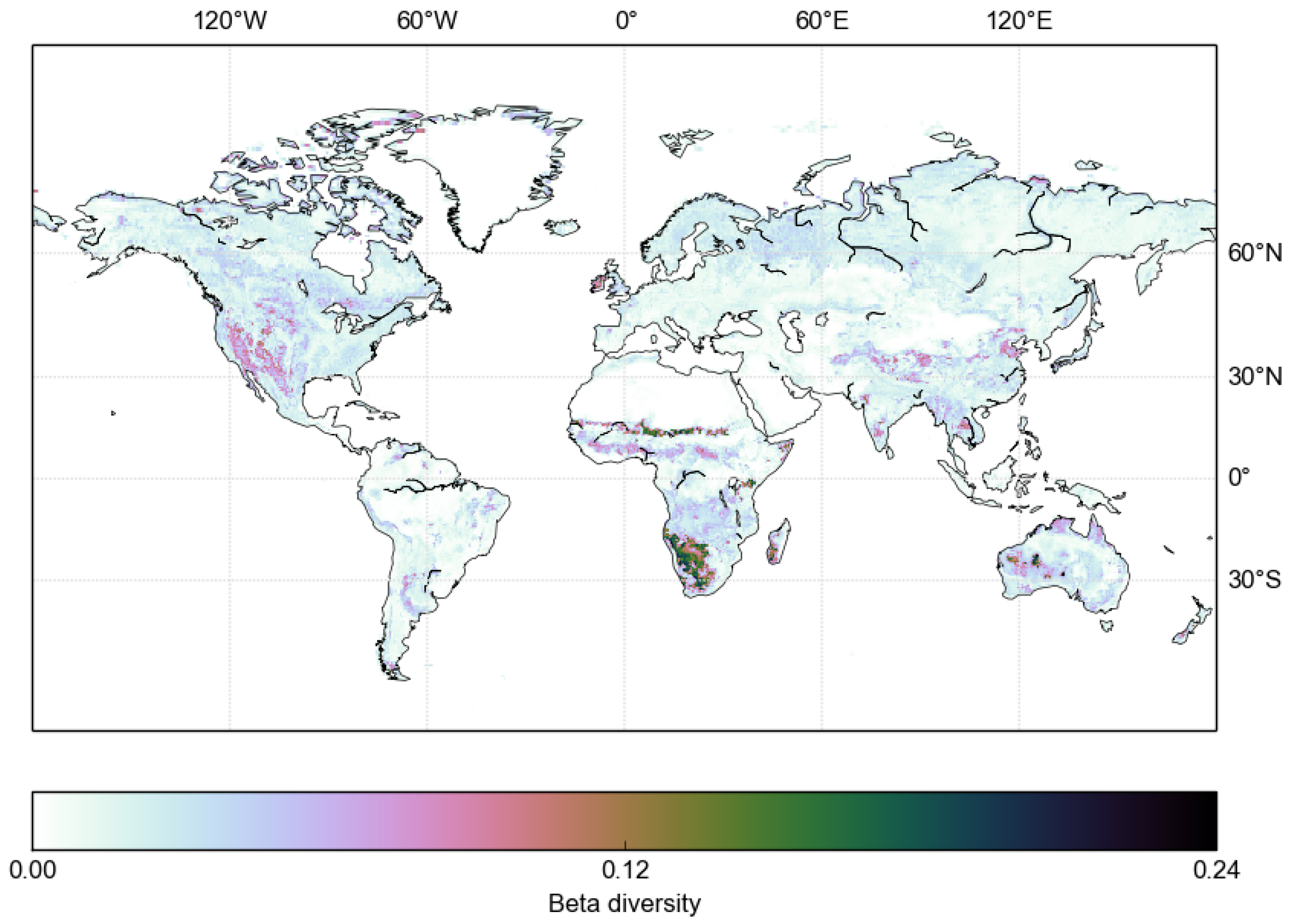
The pattern of uncertainties evident in the beta diversity shown in Figure 6 is controlled by two factors: (1) the magnitude of the uncertainty of the classes present at any given point, and the degree to which they are confused with each other (
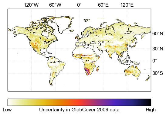
i.e., according to the confusion matrix) and; (2) the actual mix of classes present—even if a very confused class is present, the classes with which it is confused must also be present for it to become uncertain. Consequently, homogeneous areas such as the Amazon forest have very low uncertainty. Parts of southern Africa exhibit very high uncertainties, and these are due to the presence of class 140 (closed to open grassland) along with other classes that it is confused with. Class 140 itself is one of the most erroneous in the original confusion matrix.
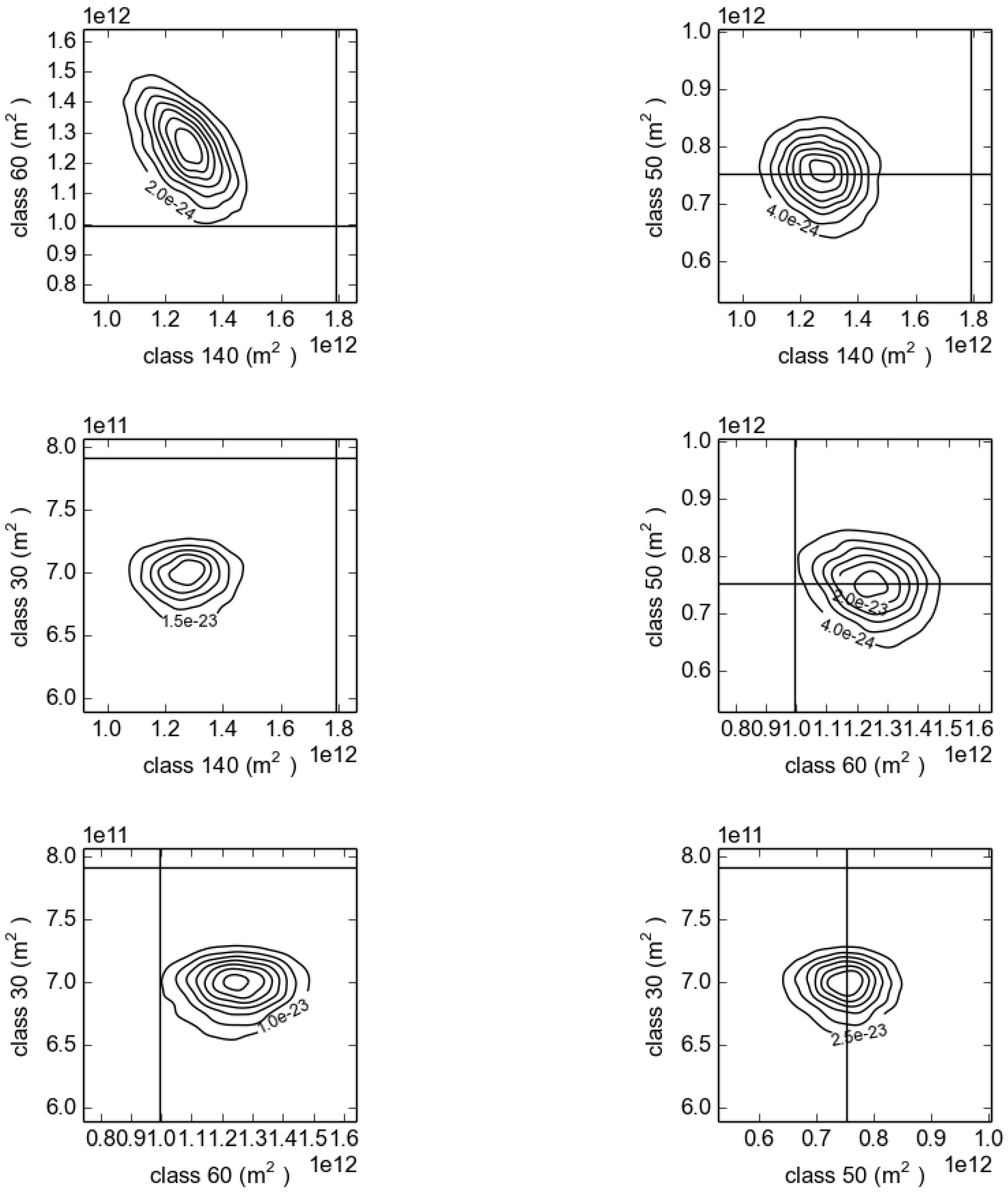
To examine the high uncertainties in southern Africa in more detail, Figure 7 shows the two-dimensional marginal probability distributions. The land cover classes represented in the figure are those that are most abundant in the region: mosaic vegetation (grassland, shrubland, forest) and cropland (30), closed broadleaved deciduous forest (50), open broadleaved deciduous forest (60), and closed to open grassland (140). Contours in these plots are lines of equal likelihood of area covered by each class, and the vertical and horizontal lines are the values calculated from the original GlobCover data. Where a line bisects the centre of the distribution, this indicates no bias between the GlobCover and the statistical model. This is only the case for class 50, which agrees with the global area distributions in Figure 5. The pattern of bias for the other classes also mimics the biases seen in the global data: classes 140 and 30 have a positive bias, whereas 60 has a negative bias. This illustrates an important shortcoming of the specific experiment presented here, rather than the technique in general. Because the uncertainty information comes from a confusion matrix that represents the whole globe, the pattern of uncertainties will be broadly the same for every location. In reality, this is not likely to be the case. This is discussed further in Section 5.2.
One interesting feature of the results that is only visible in Figure 7 is that some of the classes exhibit covariance. The most obvious example is the negative correlation between class 140 and class 60. In this case, a negative correlation implies that an error in one land class will correspond to an error in the opposite direction in the other. This can be seen in the global posterior distributions (Figure 5), where the bias in the global area of classes 140 and 60 is in the opposite direction.

5.2. Assumptions and Limitations

One key assumption in the method presented in this paper is that the confusion matrix describes classification uncertainties that do not vary spatially. For example, confusion between grasses and crops is taken to be the same regardless of whether this occurs in, say, the United Sates or Asia. This may not hold true for two principal reasons: first, the amount and quality of data may not be the same from location to location (due to orbital characteristics and variable amount of clouds, for example) and second, because the spectral characteristics of a specific land cover may be different (for example, due to different soil types). In principle, it is possible to extend the method to cope with a spatially varying confusion matrix. The simplest way of achieving this being to have several regional confusion matrices, or matrices which are built from ground samples within a given range of a grid–cell. However, either of these approaches would need a much larger validation data set and is beyond the scope of this study.
Some cover types are poorly sampled in the confusion matrix, which is likely to make the results for these classes less reliable. Again, the only solution is to produce confusion matrices with larger numbers of observations. Practically this is very time consuming and resource intensive for global maps of this nature, and consequently requires coordinated input from relevant agencies. A recommendation from this paper is that such activities require a greater level of funding.

5.3. The Role of the Prior

In many ways, the maps of uncertainty produced can be viewed as a spatialisation of the confusion matrix. So what role does the prior play? To calculate Bayesian estimates of any quantity necessarily requires a prior estimate, and these are often subjective in nature. Prior information in this paper comes from a spatially smoothed version of the land cover map consisting of a 1 . 5 × 1 . 5 moving average. Larger windows up to 5 . 5 × 5 . 5 were tried and showed only marginal difference (results not shown). The same spatial patterns in uncertainty and distributions of bias in global areas were observed. One example of an alternative prior might be to use some estimate of the grid–cell heterogeneity in land cover (e.g., how “patchy” the landscape is). A less ad-hoc alternative would be to use the inherent information available in the classification procedure itself. There are a number of metrics, such as fuzzy classifications, typically based on measures of spectral separability between classes, that assign probabilities of membership of each pixel to a given land cover class. These may be a more informative prior for the statistical model used here. This information is not generally made available for global land cover products such as GlobCover, but the approach merits further investigation as a means of combining the spectral and validation data into a single estimate of uncertainty.
One important role that the prior plays in this study is that it excludes classes that are not present in the local region. To illustrate with an extreme example: the bare areas class (200) exhibits a small amount of confusion with permanent snow and ice (220). Based on the confusion matrix alone this would mean that there is a small probability of snow and ice existing anywhere that bare areas appear, including the Sahara desert. Clearly this is not desirable. However, because the prior contains zero proportion of class 220 in this region, it means that the posterior probability for it is also zero.

5.4. Application to Modelling

This paper has only demonstrated the application of the technique as far as producing posterior estimates of uncertainty from a land cover product. However, the motivation of this study is ultimately to provide a technique that will allow these uncertainties to be propagated through any environmental model that uses land cover data as an input, such as the Sheffield Dynamic Vegetation Model, SDGVM [20], or the Joint UK Land Environment Simulator, JULES [26]. An important part of this process that has not been considered in this paper is the conversion of land cover as represented in a remotely sensing product to the classes required by the models (typically called plant functional types). This is likely to have two main impacts: either where a PFT contains multiple land cover classes, or where a land cover class contains multiple PFTs. The first is likely to reduce uncertainty in the model predictions due to the land cover uncertainty, whereas the second will increase uncertainty. Further studies will look at the propagation of the derived uncertainties through such models to examine the impact on predictions of, for example, carbon and energy fluxes between the land surface and the atmosphere. Clearly the most important question to ask is not how much error there is in a given land cover product, but how this will impact a given application. Such experiments are computationally intensive and beyond the scope of this paper; future studies will address this issue.
The process by which the uncertainty estimates presented here can be propagated by a model is simple and requires no modification to the model. The sampler presented in Section 3 is capable of producing an unlimited number of realisations of the true land cover. Each of these realisations can then be used as an instance of the land cover (or PFTs) for a model run, using as many runs as necessary to calculate the required statistics. Typically this could be between 100’s to 10000’s of model runs. The uncertainty in model predictions due to uncertainty in the land cover can then be calculated using the ensemble of model outputs that has been generated.

6. Conclusions

This paper applies a method of drawing samples from the posterior distribution of land cover proportions implied by the GlobCover 2009 global land cover data set and an associated uncertainty matrix. The method is designed to handle large data sets and was able to provide measures of uncertainty in the GlobCover 2009. The results highlight both the specific classes and the geographical regions in which the land cover product performs either poorly or well. Geographically, most uncertainty is seen in southern Africa (Figure 6), in which exists a complex heterogeneous landscape consisting of shrubs and grass. In particular, this uncertainty is driven by the presence of a specific class (140) within this landscape. The largest overall biases in areal coverage reported by the GlobCover product shown in Figure 5 are dominated by non-vegetated surfaces: bare areas, inland water bodies, and artificial surfaces. The largest biases in vegetation occur post-flooding or irrigated cropland and the two mosaic cropland/vegetation classes. Overall, however, the analysis shows the GlobCover 2009 product to be of high accuracy: biases for most classes are small, and PDFs are relatively narrow.
Future work is planned to propagate these uncertainties through a Global Vegetation Model to demonstrate the impacts on model predictions of the net carbon balance of the land surface. As part of this, it will also be necessary to address the uncertainties in the cross-walk between land cover and plant functional types; however, the work outlined here lays the foundation for this analysis. Although the focus in this study has been preparing to work with Global Vegetation Models, in principle the technique can be used for any model that requires land cover as an input—for example, climate models or hydrological models.
A strong recommendation arising from this work is that more funding is required to produce accuracy assessments of land cover products. With a greater level of sampling in the confusion matrix it would be possible to apply the method presented here on a regional level and ultimately provide more detailed analysis to inform onward use of the data. In addition, some classes are under-represented in the existing confusion matrix, and uncertainty estimates generated for these will be the least reliable.

Acknowledgments

Thanks go to the anonymous reviewers and the Editor of the Special Issue whose comments and suggestions helped strengthen this paper. Quaife’s contribution to this work was funded by the UK NERC National Centre for Earth Observation. A software implementation of the statistical model and the 10000 generated land cover map instances from the GlobCover 2009 product (at 1 2 degree resolution) are available from the corresponding author. The software is written in C and depends on the GNU Scientific Library. Computer code for the statistical model is available at: https://github.com/tquaife/bayesLC.

Author Contributions

Quaife implemented the statistical model and performed the runs presented in this paper. Cripps developed the theoretical aspects of the model. Both authors contributed to the production of the manuscript.

Conflicts of Interest

The authors declare no conflict of interest.

References

  1. Friedl, M.A.; McIver, D.K.; Hodges, J.C.; Zhang, X.; Muchoney, D.; Strahler, A.H.; Woodcock, C.E.; Gopal, S.; Schneider, A.; Cooper, A.; et al. Global land cover mapping from MODIS: Algorithms and early results. Remote Sens. Environ. 2002, 83, 287–302. [Google Scholar] [CrossRef]
  2. Friedl, M.A.; Sulla-Menashe, D.; Tan, B.; Schneider, A.; Ramankutty, N.; Sibley, A.; Huang, X. MODIS collection 5 global land cover: Algorithm refinements and characterization of new datasets. Remote Sens. Environ. 2010, 114, 168–182. [Google Scholar] [CrossRef]
  3. Bartholomé, E.; Belward, A. GLC2000: A new approach to global land cover mapping from Earth observation data. Int. J. Remote Sens. 2005, 26, 1959–1977. [Google Scholar] [CrossRef]
  4. Bontemps, S.; Defourny, P.; Van Bogaert, E.; Arino, O.; Kalogirou, V.; Ramos Perez, J. GlobCover 2009: Products Description and Validation Report. 2011. Available online: http://ionia1.esrin.esa.int/docs/GLOBCOVER2009_Validation_Report_2 (accessed on 1 November 2016).
  5. Arino, O.; Bicheron, P.; Achard, F.; Latham, F.; Witt, R.; Weber, J.L. The most detailed portrait of Earth. ESA Bull. 2008, 136, 25–31. [Google Scholar]
  6. Oleson, K.W.; Bonan, G.B. The effects of remotely sensed plant functional type and leaf area index on simulations of boreal forest surface fluxes by the NCAR land surface model. J. Hydrometeorol. 2000, 1, 431–446. [Google Scholar] [CrossRef]
  7. Steyaert, L.; Hall, F.; Loveland, T. Land cover mapping, fire regeneration, and scaling studies in the Canadian boreal forest with 1 km AVHRR and Landsat TM data. J. Geophys. Res. 1997, 102, 29581–29598. [Google Scholar] [CrossRef]
  8. Desai, A.R.; Moore, D.J.P.; Ahue, W.K.M.; Wilkes, P.T.V.; De Wekker, S.F.J.; Brooks, B.G.; Campos, T.L.; Stephens, B.B.; Monson, R.K.; Burns, S.P.; et al. Seasonal pattern of regional carbon balance in the central Rocky Mountains from surface and airborne measurements. J. Geophys. Res. Biogeosci. 2011, 116. [Google Scholar] [CrossRef]
  9. Woodward, F.; Lomas, M.; Quaife, T. Global responses of terrestrial productivity to contemporary climatic oscillations. Philos. Trans. R. Soc. B Biol. Sci. 2008, 363, 2779–2785. [Google Scholar] [CrossRef] [PubMed]
  10. Poulter, B.; Frank, D.C.; Hodson, E.L.; Zimmermann, N.E. Impacts of land cover and climate data selection on understanding terrestrial carbon dynamics and the CO2 airborne fraction. Biogeosciences 2011, 8, 2027–2036. [Google Scholar] [CrossRef]
  11. Schimel, D.S.; House, J.; Hibbard, K.; Bousquet, P.; Ciais, P.; Peylin, P.; Braswell, B.H.; Apps, M.J.; Baker, D.; Bondeau, A.; et al. Recent patterns and mechanisms of carbon exchange by terrestrial ecosystems. Nature 2001, 414, 169–172. [Google Scholar] [CrossRef] [PubMed]
  12. DeFries, R.S.; Field, C.B.; Fung, I.; Justice, C.O.; Los, S.; Matson, P.A.; Matthews, E.; Mooney, H.A.; Potter, C.S.; Prentice, K.; et al. Mapping the land surface for global atmosphere-biosphere models: Toward continuous distributions of vegetation’s functional properties. J. Geophys. Res. 1995, 100, 20867–20882. [Google Scholar] [CrossRef]
  13. Hansen, M.; DeFries, R.; Townshend, J.; Carroll, M.; Dimiceli, C.; Sohlberg, R. Global percent tree cover at a spatial resolution of 500 meters: First results of the MODIS vegetation continuous fields algorithm. Earth Interact. 2003, 7, 1–15. [Google Scholar] [CrossRef]
  14. Schuh, A.; Denning, A.; Corbin, K.; Baker, I.; Uliasz, M.; Parazoo, N.; Andrews, A.; Worthy, D. A regional high-resolution carbon flux inversion of North America for 2004. Biogeosciences 2010, 7, 1625–1644. [Google Scholar] [CrossRef]
  15. Werner, C.; Butterbach-Bahl, K.; Haas, E.; Hickler, T.; Kiese, R. A global inventory of N2O emissions from tropical rainforest soils using a detailed biogeochemical model. Glob. Biogeochem. Cycles 2007, 21. [Google Scholar] [CrossRef]
  16. Foody, G.M. Status of land cover classification accuracy assessment. Remote Sens. Environ. 2002, 80, 185–201. [Google Scholar] [CrossRef]
  17. Maselli, F.; Conese, C.; Petkov, L. Use of probability entropy for the estimation and graphical representation of the accuracy of maximum likelihood classifications. ISPRS J. Photogramm. Remote Sens. 1994, 49, 13–20. [Google Scholar] [CrossRef]
  18. Tchuenté, A.T.K.; Roujean, J.L.; De Jong, S.M. Comparison and relative quality assessment of the GLC2000, GLOBCOVER, MODIS and ECOCLIMAP land cover data sets at the African continental scale. Int. J. Appl. Earth Obs. Geoinform. 2011, 13, 207–219. [Google Scholar] [CrossRef]
  19. Quaife, T.; Quegan, S.; Disney, M.; Lewis, P.; Lomas, M.; Woodward, F. Impact of land cover uncertainties on estimates of biospheric carbon fluxes. Glob. Biogeochem. Cycles 2008, 22. [Google Scholar] [CrossRef]
  20. Woodward, F.; Lomas, M. Vegetation dynamics—Simulating responses to climatic change. Biol. Rev. 2004, 79, 643–670. [Google Scholar] [CrossRef] [PubMed]
  21. Poulter, B.; Ciais, P.; Hodson, E.; Lischke, H.; Maignan, F.; Plummer, S.; Zimmermann, N.E. Plant functional type mapping for earth system models. Geosci. Model Dev. 2011, 4, 993–1010. [Google Scholar] [CrossRef]
  22. Green, E.; Strawderman, W. Determining the accuracy of thematic maps. Statistician 1994, 43, 77–85. [Google Scholar] [CrossRef]
  23. Denham, R.; Mengersen, K.; Witte, C. Bayesian analysis of thematic map accuracy data. Remote Sens. Environ. 2009, 113, 371–379. [Google Scholar] [CrossRef]
  24. Cripps, E.; O’Hagan, A.; Quaife, T. Quantifying uncertainty in remotely sensed land cover maps. Stoch. Environ. Res. Risk Assess. 2013, 27, 1239–1251. [Google Scholar] [CrossRef]
  25. Conese, C.; Maselli, F. Use of error matrices to improve area estimates with maximum likelihood classification procedures. Remote Sens. Environ. 1992, 40, 113–124. [Google Scholar] [CrossRef]
  26. Best, M.; Pryor, M.; Clark, D.; Rooney, G.; Essery, R.; Ménard, C.; Edwards, J.; Hendry, M.; Porson, A.; Gedney, N.; et al. The Joint UK Land Environment Simulator (JULES), model description—Part 1: Energy and water fluxes. Geosci. Model Dev. 2011, 4, 677–699. [Google Scholar] [CrossRef]
Figure 1. The proportion of six land cover classes as recorded in the GlobCover2009 data: (a) class 14; (b) class 40; (c) class 90; (d) class 130; (e) class 140 and (f) class 150. Class definitions are given in Table 1.
Remotesensing 08 00314 g001
Figure 2. The posterior estimate (mean) of the proportion of six land cover classes: (a) class 14; (b) class 40; (c) class 90; (d) class 130; (e) class 140 and (f) class 150. Class definitions are given in Table 1.
Remotesensing 08 00314 g002
Figure 3. The modelled uncertainty, approximated by the posterior standard deviation, in six land cover classes: (a) class 14; (b) class 40; (c) class 90; (d) class 130; (e) class 140 and (f) class 150. Class definitions are given in Table 1.
Remotesensing 08 00314 g003
Figure 4. Scatter plots of land cover proportion reported in the GlobCover product against the mean of the posterior. The classes are (a) class 14; (b) class 40; (c) class 90; (d) class 130; (e) class 140 and (f) class 150. The x–axis is the original data and the y–axis is the output from the statistical model.
Remotesensing 08 00314 g004
Figure 5. The modelled posterior PDF in the total area covered by each land cover type. Vertical dashed lines show the corresponding totals from the Glob Cover product itself. Class definitions are given in Table 1.
Remotesensing 08 00314 g005
Figure 6. Uncertainty in the GlobCover data as represented by the beta diversity for all classes.
Remotesensing 08 00314 g006
Figure 7. 2D marginal posterior distributions for southern Africa. Axis labels indicate the land cover class, and contour values are the likelihoods that each contour corresponds to. The axes themselves show total area covered by the class in m 2 . The vertical and horizonatal lines show the areas predicted areas from the original data.
Remotesensing 08 00314 g007
Table 1. Land cover classes represented in the GlobCover 2009 product. N refers to the total number of samples of that class in the reference data. P refers to the producer’s accuracy (%). U refers to the user’s accuracy (%).
IDNPUDescription
11782473Post-flooding or irrigated croplands
144023567Rainfed croplands
202010012Mosaic Cropland (50%–70%)/Vegetation (grassland, shrubland, forest) (20%–50%)
30121008Mosaic Vegetation (grassland, shrubland, forest) (50%–70%)/Cropland (20%–50%)
403447288Closed to open (>15%) broadleaved evergreen and/or semi-deciduous forest (>5 m)
50896040Closed (>40%) broadleaved deciduous forest (>5 m)
60223214Open (15%–40%) broadleaved deciduous forest (>5 m)
70684140Closed (>40%) needleleaved evergreen forest (>5 m)
90485029Open (15%–40%) needleleaved deciduous or evergreen forest (>5 m)
100512525Closed to open (>15%) mixed broadleaved and needleleaved forest (>5 m)
11051006Mosaic Forest/Shrubland (50%–70%)/Grassland (20%–50%)
12031004Mosaic Grassland (50%–70%)/Forest/Shrubland (20%–50%)
1302292944Closed to open (>15%) shrubland (<5 m)
1402131831Closed to open (>15%) grassland
150975935Sparse (>15%) vegetation (woody vegetation, shrubs, grassland)
16065014Closed (>40%) broadleaved forest regularly flooded—Fresh water
17087555Closed (>40%) broadleaved semi-deciduous and/or evergreen forest regularly
flooded—Saline water
180302339Closed to open (>15%) vegetation (grassland, shrubland, woody vegetation) on
regularly flooded or waterlogged soil—Fresh, brackish, or saline water
190452069Artificial surfaces and associated areas (urban areas >50%)
2002466988Bare areas
2101107093Water bodies
220446883Permanent snow and ice
Table 2. The “certain” and “heterogeneous” confusion matrix for the GlobCover 2009 product.
Class ID111420304050607090100110120130140150160170180190200210220
11194 12
1429141 71 9112 1154
20107520 11321 3 12143 72
30658 121211 1 172131 125 1
40216 24931 1 81 1 1
50 17 205326212 153 1 11
60 11 1027 1 1431 2
70 3 2222864 95 13131
901 13217244 7112 3 251
100 1 19 8113 68 2 2
110 14 12 125 18204 1138
12018 2 162 317165 2 5
130124 127231 66192 15213
140124 3114 203812 26111
150 4 1 362 53057 2429137
160 16 1 3 1
1701 1 162
1801 1 15 7 3
19011 1 91
20031 1 356 116911
2102 2 277
220 1 1430

