A Multi-View Dense Point Cloud Generation Algorithm Based on Low-Altitude Remote Sensing Images

Abstract

This paper presents a novel multi-view dense point cloud generation algorithm based on low-altitude remote sensing images. The proposed method was designed to be especially effective in enhancing the density of point clouds generated by Multi-View Stereo (MVS) algorithms. To overcome the limitations of MVS and dense matching algorithms, an expanded patch was set up for each point in the point cloud. Then, a patch-based Multiphoto Geometrically Constrained Matching (MPGC) was employed to optimize points on the patch based on least square adjustment, the space geometry relationship, and epipolar line constraint. The major advantages of this approach are twofold: (1) compared with the MVS method, the proposed algorithm can achieve denser three-dimensional (3D) point cloud data; and (2) compared with the epipolar-based dense matching method, the proposed method utilizes redundant measurements to weaken the influence of occlusion and noise on matching results. Comparison studies and experimental results have validated the accuracy of the proposed algorithm in low-altitude remote sensing image dense point cloud generation.

1. Introduction

With the development of laser scanning and image matching technology, three-dimensional (3D) information has increasingly attracted researchers’ attention. Applications of 3D information have extended from digital elevation model (DEM) and digital surface model (DSM) generation to many other fields including archeology [1,2], topographic monitoring [3,4], facial geometry and dynamic capture [5,6], cultural heritage protection [7,8], forest and agriculture modeling [9,10], and medical treatment [11]. Since laser scanning can produce highly accurate, reliable, dense, and more integrated 3D point clouds of objects [12], it has been utilized as the preferred technology for 3D modeling over the last two decades. In recent years, with the significant progress of photogrammetry and computer vision technology, image-based 3D reconstruction stands as a major competitor against laser scanning [13]. Compared with laser scanning, the advantages of image-based 3D reconstruction are that:

• Images can be accepted from any type of camera [14], including calibrated or uncalibrated images, images taken from smartphones or tablets [15], images captured from digital cameras or frames intercepted from video streams [16];
• It is low in cost;
• Point cloud data contains color information; and
• Theoretically, it may produce much denser point clouds [17].

In numerous photographic platforms, low-altitude remote sensing images have been considered a popular data source for large-scale 3D modeling [18]. In addition to sub-decimeter high-resolution imagery [19], a low-altitude remote sensing platform also has several advantages including: flexibility, low cost, simplicity of operation, and ease of maintenance [20].

This paper proposes a multi-view dense point cloud generation algorithm based on low-altitude remote sensing images. The proposed method exploited Patch-based Multi View Stereo (PMVS) [21] results as a seed point cloud. It took advantage of pixels in image windows and object points on patches to expand the seed point cloud. Then, it utilized multi-image projection relationships to improve the accuracy of the point cloud. In summary, the purpose of this paper is a new approach that takes advantage of redundant measurements of multi-images and generates a much denser point cloud than MVS.

The remainder of the paper is structured as follows: related works are presented and compared with each other in Section 2; in Section 3, the proposed method is introduced in detail; in Section 4, experiments are conducted to verify the feasibility of the proposed algorithm in terms of reliability and matching accuracy; and finally, conclusions are stated in Section 5.

2. Related Works

The theory of stereo matching was first investigated in the early mid-1970s [22] and underwent extensive development in the 1990s [17]. During those 10 years, a large number of high accuracy matching applications and commercial photogrammetric systems appeared for digital surface model (DSM) and digital terrain model (DTM) generation from aerial images. In the last decade, image-based 3D reconstruction approaches have been further advanced by recent developments in computer vision and photogrammetry. Additionally, the data source of images has been extended from satellite aerial images to generic photos, such as those taken on mobile photos.

2.1. Two-Frame Dense Matching in Photogrammetry

Since the advent of stereo matching, the derivation of ground object point coordinates from corresponding image pixels has become one of the most key issues in the domain of photogrammetry and remote sensing [23,24]. With the advances of hardware and innovative image matching algorithms, photogrammetry-based 3D modeling can deliver results in a reasonable amount of time. Some researchers have focused on how to utilize photogrammetry technology to produce relatively sparse seed points [25,26], while others have sought to take advantage of the corresponding epipolar lines between two corresponding images to perform pixel-wise dense matching [27,28,29]. In 2002, Scharstein and Szeliski [27] introduced a taxonomy and evaluation of two-frame stereo dense matching algorithms, dividing it into four primary steps:

• Matching cost computation;
• Cost (support) aggregation;
• Disparity computation/optimization; and
• Disparity refinement.

Based on the implementation employed in the cost (support) aggregation step, dense matching can be divided into two categories: local algorithms and global algorithms. Local algorithms connect the matching costs within a local neighborhood and select the lowest matching cost as a disparity [30], that is “winner takes all′′. Global algorithms typically define a global energy function which includes a data term and a smoothness term acting on the whole image instead of local cost aggregations [31]. Since the local algorithm uses a part of the local neighborhood for calculations, the processing speed of the local algorithm is faster, and due to the global algorithms taking into account the whole image in processing, the matching accuracy of the global algorithms is greater. Hirschmüller [32] employed Semi-Global Matching (SGM) which integrates the advantages of local and global algorithms and further improved the efficiency and accuracy of dense matching. Despite these advantages, the two-frame method could not evade the key problem that without the redundant measurements, two-frame dense matching was not robust to the noise and occlusion, and the accuracy of the point cloud reconstructed by two-frame matching is inferior to that of multi-view stereo [33].

2.2. Multi-View Stereo in Computer Vision

With the development of a number of different low-cost and open-source software systems, the multi-view stereo method is becoming one of the most popular subjects in computer vision. Multi-view stereo can use redundant information to weaken the influence of occlusion and noise. From the Middlebury evaluation supplied by Seitz et al. [34], for a single object or small-scale sense reconstruction, multi-view reconstruction can provide a first-rate result which is comparable to the point cloud obtained from laser scanning. Since the Structure from Motion (SFM) method makes it possible for disordered image calibration, multi-view stereo quickly extends from photogrammetric images to generic photos, even those downloaded from the Internet or captured from mobile phones [35]. Recently, the challenges of multi-view stereo have focused on the following aspects:

• dynamic capture;
• 3D reconstruction from video streams; and
• 3D reconstruction for large-scale scenes.

For large-scale scene reconstruction, although there are plenty of efforts devoted to making point cloud data denser and more accurate, the density and accuracy of the result cannot substitute the laser scanning point cloud. Since low-altitude remote sensing images have many advantages such as flying under the cloud, low cost and fast response, etc., this article focuses on how to apply low-altitude remote sensing images to reconstruct large-scale scenes.

3. Method

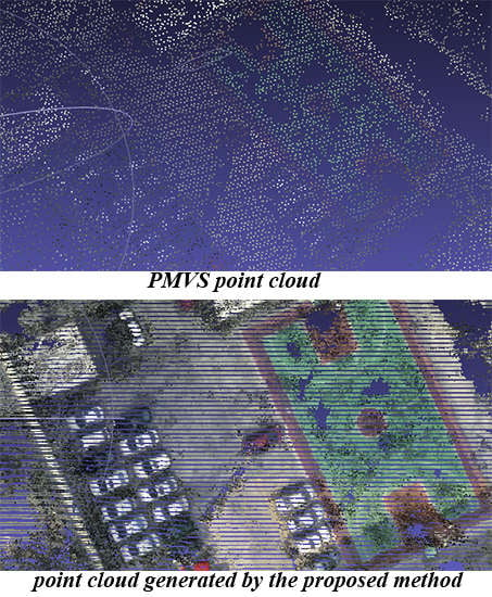
The proposed method can be divided into four steps: (1) a PMVS point cloud generation; (2) patch-based point cloud expansion; (3) point cloud optimization; and (4) an outliers filter. In this section, details of the proposed method are introduced. The principle of this algorithm is illustrated in Figure 1. As shown in Figure 1, the proposed method derives from a technique where growing regions start from a set of seed points or patches [36]. The result of PMVS is a set of patches, and the geometric significance of the patch is a local tangent plane of the object. The proposed algorithm utilizes these results as seed points and takes advantage of projection rules between image pixels and patches to segment the generated patches to expand denser patches. Then, a patch-based Multiphoto Geometrically Constrained Matching (MPGC) algorithm is used to optimize the expanded patches to obtain a more accurate result. Finally, a density constraint [37] is employed to filter the outliers.

3.1. PMVS Point Cloud Generation

In recent years, many researchers have focused on using MVS to reconstruct large-scale 3D scenes. PMVS is accepted as one of the most popular MVS algorithms due to its accuracy and completeness [8]. By utilizing (1) initial feature matching; (2) patch expansion; and (3) patch filtering, PMVS generates and propagates a semi-dense set of patches [38]. In contrast to a feature-based algorithm, the seed points generated by PMVS have three advantages:

• Much denser: seed points obtained in feature-based matching are expanded in the second step of PMVS;
• Evenly distributed: the PMVS algorithm attempted to reconstruct at least one patch in each image cell with β × β pixels;
• More accurate: a Nelder-Mead method [39] was utilized in the PMVS algorithm to refine each patch in the reconstruction model and filter outliers in the last step.

3.2. Patch-Based Point Cloud Expansion

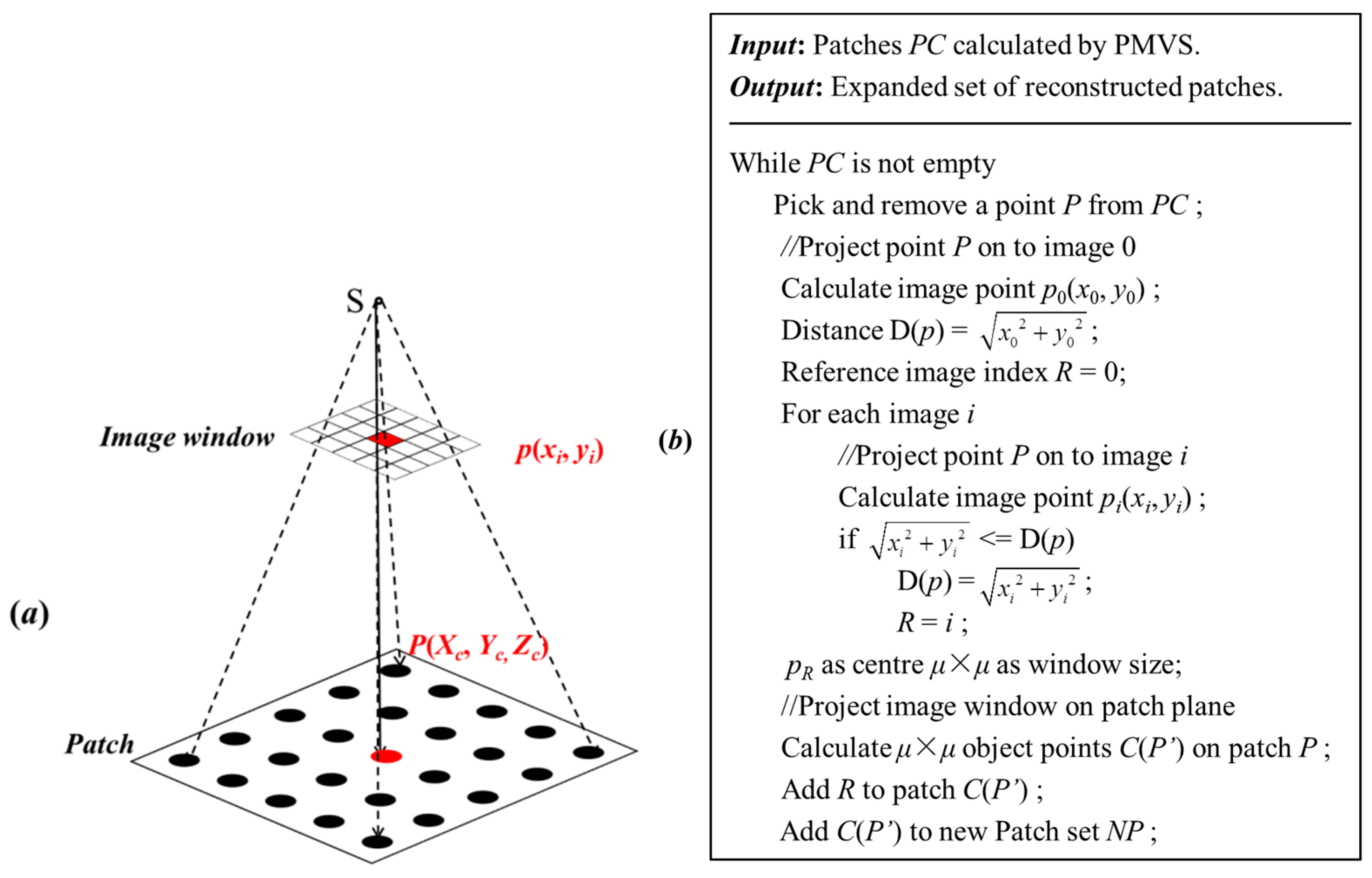
The goal of the expansion step is to expand the seed patch and increase the point cloud density. PMVS attempted to grow a patch starting from a seed matching pixels, and expanding to the neighbor image cells in the visible images until each corresponding image cell reconstructed at least one point. The proposed method utilizes the projection rules to segment the patches into small pieces. Each piece contains one center point, the seed point is growing on the patch and the point cloud is denser.

The result of PMVS records each point in the point cloud with its coordinates (X_c, Y_c, Z_c), color (R, G, B) and normal vector (a, b, c). By projecting the object point P(X_c, Y_c, Z_c) on each image, the image point coordinate p_i(x_i, y_i) (i is the image index) is calculated. Since the distance between the image point and the origin of the image coordinate system is shorter, the projection distortion is smaller, and the proposed method supposes image I(R) as a reference image when the image I(R) is satisfied by:

$$\sqrt{{x_R}^2+{y_R}^2}\le \sqrt{{x_i}^2+{y_i}^2}(i=1,\mathrm{2...}n,i\ne R)$$

(1)

Supposing (X_c, Y_c, Z_c) is the center of the patch, and (a, b, c) is the normal vector, the local tangent plane (patch in PMVS) at P(X_c, Y_c, Z_c) is:

$$P:a\left(X-X_c\right)+b\left(Y-Y_c\right)+c\left(Z-Z_c\right)=0$$

(2)

As illustrated in Figure 2a, the image point p_i(x_i, y_i) is the center of the image window, where the window size is μ × μ pixels. By projecting the image window onto the patch, μ × μ object points are obtained. Theoretically, the density of the point cloud could expand μ × μ times. The overall algorithm description for this step is given in Figure 2b. The result patch P′ consists of the coordinates (X, Y, Z), normal vector (a, b, c) and reference image index R.

3.3. Patch-Based MPGC to Optimize the Point Cloud

PMVS utilized the projection relationship between the patch and the corresponding images to build a function to find the optimal matching pixel:

$$f(z,\alpha ,\beta )=\frac{1}{n}{\displaystyle \sum _{i=1}^n(1-f_i)}$$

(3)

In the function above, i is the index of the visible images (in PMVS, if patch p is visible in image i, i is considered as a visible image of p); n is the number of the visible images; f_i is a function that denotes the Normalized Cross-correlation Coefficient (NCC) between corresponding image windows which is obtained by the patch projecting to the reference image (I₀) and visible images (I_i);

$$f_i(z,\alpha ,\beta )=NCC(I_0,I_i)$$

(4)

z is the distance of the patch center moving along the ray; (α, β) are the direct angle of the normal vector (a, b, c). The optimization process employed the Nelder-Mead method [39] to calculate the minimum value of Function (3). From the result of the calculation, the optimal patch (denoted by its center point P′ and normal vector (a, b, c)) is obtained:

$$P^{\prime }=P+z\cdot norm(\overrightarrow{OP})$$

(5)

$$\begin{array}{l}a=cos\alpha cos\beta \\ b=sin\alpha cos\beta \\ c=sin\beta \end{array}$$

(6)

As with the optimization method in PMVS, the proposed method also introduces a patch in the optimization step to obtain a better initial value of the optimization function. In the 1990s, Baltsavias [40,41] introduced epipolar line constraints (collinear equation) to Least Square Image Matching (LSM) [42,43] and proposed an extremely useful application named Multi-photo Geometrically Constrained Matching (MPGC). This approach simultaneously derives the accurate coordinates of corresponding object points in the object space coordinate system during the image matching process. It has been widely applied to refine matching results in a three-dimensional reconstruction [25,26,44,45]. The proposed method utilizes a modified MPGC algorithm to optimize the point cloud.

In the traditional LSM method, each pixel in the matching image window is used to build an error equation:

$$v=d{h}_{0i}+g_i\left(x_i,y_i\right)\cdot d{h}_{1i}+h_{1i}\left(\frac{\partial g_i}{\partial x_i}d{x}_i+\frac{\partial g_i}{\partial y_i}d{y}_i\right)-\left(g_0\left(x_0,y_0\right)-h_{0i}-h_{1i}\cdot g_i\left(x_i,y_i\right)\right)$$

(7)

In the error equation above, v is the projection error; h_0i and h_1i are the radiation distortion coefficients between the reference image and search image i. In the experiments, the initial values of h_0i and h_1i are usually 0 and 1, respectively. Further, dh_0i and dh_1i are corrections of parameter h_0i and h_1i; g₀(x₀, y₀) is the pixel intensity values in the image window of the reference image; g_i(x_i, y_i) is the pixel intensity values of image points (x_i, y_i) in the search image window; (∂g_i/∂x_i, ∂g_i/∂y_i) is the derivative values of pixel intensity in the x and y directions; (dx_i, dy_i) is the correction values of the image points (x_i, y_i). Therefore, in a matching of the μ × μ pixels image window, the μ × μ error equations can be listed; if μ × μ is larger than the unknown, using least square adjustment, the corresponding pixels (x_i, y_i) can be calculated.

MPGC applied epipolar line constraints to the LSM method, and the coordinates of (x_i, y_i) can be denoted by the interior (x_s, y_s, f) and exterior parameters (projection center S(X_s, Y_s, Z_s), rotation matrix (a₁, a₂, a₃; b₁, b₂, b₃; c₁, c₂, c₃)) of image i and the corresponding object point (X, Y, Z):

$$\begin{array}{l}{x}_i-x_s=-f\frac{a_1\left(X-X_s\right)+b_1\left(Y-Y_s\right)+c_1\left(Z-Z_s\right)}{a_3\left(X-X_s\right)+b_3\left(Y-Y_s\right)+c_3\left(Z-Z_s\right)}\\ y_i-y_s=-f\frac{a_2\left(X-X_s\right)+b_2\left(Y-Y_s\right)+c_2\left(Z-Z_s\right)}{a_3\left(X-X_s\right)+b_3\left(Y-Y_s\right)+c_3\left(Z-Z_s\right)}\end{array}$$

(8)

Applying the collinear Equation (8) to the LSM error Equation (7), the optimal object point coordinate can be directly obtained during the process of least square adjustment.

However, despite the fact that MPGC performs well in matching refinement, how to select the initial matching window is still a challenge that has yet to be overcome, because either the accuracy of the result or the efficiency of the process is reliant on the quality of the initial value. The proposed method introduces the patch to MPGC to refine the point cloud. By using the patch set obtained in Section 3.2 as an initial value and projecting each patch onto the visible images to get the initial matching image windows, these initial matching windows have two superior qualities:

• All pixels which are located at the same place in the image matching window between the reference and search images are approximate corresponding pixels.
• Normal vectors in PMVS results as initial normal vectors of the patch plane, by projecting the patch points onto the images which can significantly decrease the projection deformation.

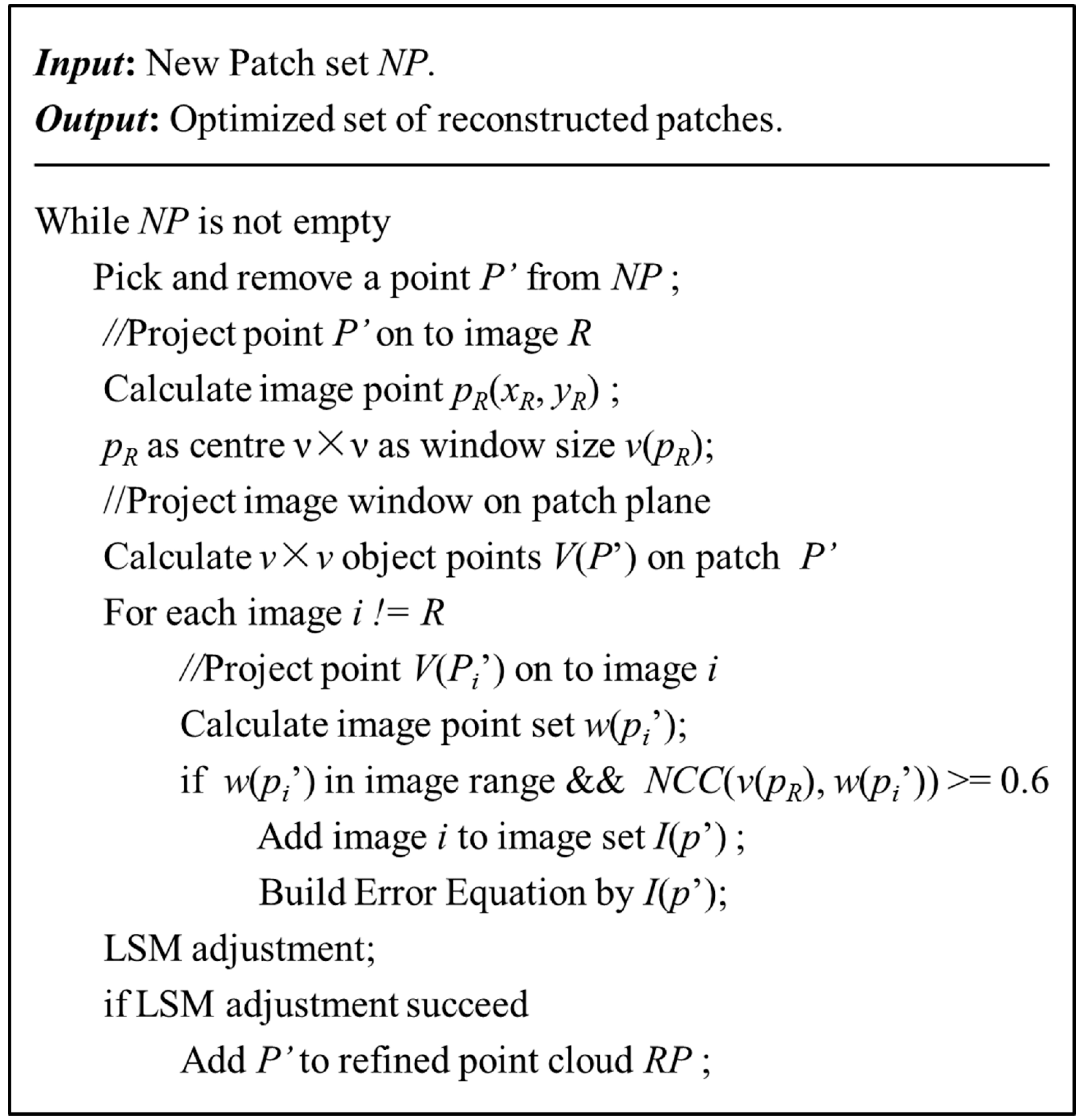
As with PMVS, the optimization algorithm in the proposed method is based on an individual patch, and each patch P′ is optimized separately in the following steps: (1) a matching window is selected in reference image R; (2) the matching window is projected onto the patch plane to calculate the corresponding object points V(P′) on patch P′; (3) V(P′) is projected onto each image except image R to obtain the corresponding points w(p_i′) on the search images; (4) if the matching window w(p_i′) is located in the range of image I and the Normalized Cross-correlation Coefficient (NCC) is larger than 0.6, then image i is collected into image set I(p′); (5) an error equation is built for each corresponding point in the image window between reference image R and search image set I(p′); (6) a least square adjustment is applied to calculate the optimal solution. The overall algorithm description for this step is illustrated in Figure 3.

The proposed method uses this patch-based MPGC algorithm to optimize the point cloud instead of the PMVS optimization method for the following reasons:

• Epipolar line constraint is the most strict constraint for a single-center projection, especially when the camera parameters are known;
• Least square adjustment can utilize redundant pixels to decrease the influence of the noise, and has a faster speed in the iterative convergence;
• Radiation distortion is taken into account.

3.4. Outliers Filter

To improve the accuracy and reduce the number of outliers in the point cloud, an erroneous point filter step is a prerequisite. The proposed method makes use of a density constraint [37] in the outliers filter step. A radius of one meter is used to compute the local neighborhood of each point. If the number of neighbor points around a center point is lower than a fixed threshold ε, the center point is considered as an outlier that should be removed. In the method of [37], ε was defined as half of the average neighbor number.

4. Experiments and Discussion

4.1. Input Data Sets

In order to evaluate the performance of the proposed method, three sets of low-altitude images were selected. Each image data set consists of five images. The data sets were captured from Northwestern University (a university in Shaanxi Province, China), Yangjiang (a city in Guangdong Province, China) and Hainan (a province in China), respectively. The parameters of the cameras (parameters of the K-matrix) were acquired from laboratory camera calibration and bundle adjustment. Commercial low altitude photogrammetric processing software called GodWork, which was developed by Wuhan University, was used to perform automatic aero-triangulation to acquire external orientation elements (parameters of the C-matrix and R-matrix) of the images. Detailed parameters of the input data sets are provided in

Table 1. The parameters of the photography from Northwest University (unmanned aerial vehicle images).

Camera Name	Area Size (m × m)	CCD Size (mm)	Image Size (pixel)	Pixel Size (μm)	Focal Length (mm)	Flying Height (m)	Ground Resolution (m)	Number of Images
Canon EOS 400D	415.8 × 339.5	22.16 × 14.77	3888 × 2592	5.7	24	600	0.118	5

,

Table 2. The parameters of the photography from Yangjiang (aerial image captured at nadir).

Camera Name	Area Size (m × m)	CCD Size (mm)	Image Size (pixel)	Pixel Size (μm)	Focal Length (mm)	Flying Height (m)	Ground Resolution (m)	Number of Images
SWDC-5	417 × 426	49.24 × 36.47	8206 × 6078	6	82	800	0.058	5

and

Table 3. The parameters of the photography from Hainan (unmanned aerial vehicle images).

Camera Name	Area Size (m × m)	CCD Size (mm)	Image Size (pixel)	Pixel Size (μm)	Focal Length (mm)	Flying Height (m)	Ground Resolution (m)	Number of Images
Canon EOS 5D	981.3 × 1004.4	36 × 24	5616 × 3744	6.4	24	650	0.174	5

, and the sample input images used in the experiments are shown in Figure 4.

4.2. Reconstructed Point Cloud

In the expansion step, expanded patch size μ is the only parameter which has to be set up, because the PMVS algorithm attempts to reconstruct at least one patch in each image cell with β × β pixels, where μ is usually less than β. From 1 to β, the density of the point cloud result is increased. Taking into account visualization and running speed, our experiments project an image window with 17 × 17 pixels on the PMVS patch and one pixel as the project interval. The comparison experiments compared the point cloud reconstructed by PMVS, SURE, Pixel4D and the proposed method. Each input data set experimented in the four comparison methods is exactly the same (same images, same camera parameters and same image parameters). The reconstructed point cloud and details are shown in Figure 5, Figure 6 and Figure 7.

As illustrated in the figures, due to the proposed method’s utilization of the PMVS result as a seed patch, the completeness of the point cloud reconstructed by PMVS and that of the proposed method are almost same. The point cloud reconstructed by the Pix4D software program has a better completeness; the point cloud reconstructed by the SURE software program was the poorest. Although SURE failed in the reconstruction of images with complex texture (i.e., the Yangjiang and Hainan data sets), for relatively simple images (the Northwestern University data set) the density of the point cloud was extremely high. From the cut figures on the right of the figure cells, it can be seen that when compared with the other three methods, the point cloud generated by the proposed method is much denser and contains more details. For instance, much plainer silhouettes and roads in the Northwestern University point cloud, cars parked on the side of the basketball court in the Yangjiang point cloud and much more meticulous roofs in the Hainan point cloud data are extracted. Detailed information of the reconstructed result is illustrated in

Table 4. Performance of dense point cloud generated by the proposed method.

Study Area	Seed Patch Number	Expanded Patch Size	Patch Number (after Expand)	Patch Number (after Filter)	Density (patches/m2)	Times (min)
Northwestern University	107514	17 × 17 (step: 2)	7890775	7802802	55.275	175
Yangjiang	324072	17 × 17 (step: 2)	24369048	24003611	135.122	627
Hainan	178317	17 × 17 (step: 2)	8481032	8474530	8.598	253

and

Table 5. Comparison of the point cloud performance.

Experimental Method	Northwestern University		Yangjiang		Hainan
	Point Number	Density (points/m2)	Point Number	Density (points/m2)	Point Number	Density (points/m2)
PMVS	107514	0.762	324072	1.824	178317	0.181
SURE	2053708	14.410	638032	3.592	770993	0.782
Pix4D	525402	3.686	2126320	11.970	1123166	1.140
The proposed method	7802802	55.275	24003611	135.122	8474530	8.598

.

The third column in Table 4 represents the experiments which used a 17 × 17 image window, and each other pixel in the image window was projected onto the patch. The computational times are recorded in the last column. All timings were obtained on a PC with Intel Core(TM) i7 3.60 GHz processors, 8 GB RAM and a 1 TB SCSI disk device for data storage, and the Microsoft Windows 7 operating system. All the processes were performed offline. From the comparison experiment results in Table 5, it can be noted that the proposed method achieves more than 40 times denser points per m² than PMVS and a more than eight times denser point cloud per m² than Pix4D. According to the image parameters and the reconstructed results, it can be seen that the density of the point cloud depends on the ground resolution of the input images. As long as the ground resolution is high enough, the proposed method can obtain much denser point clouds than laser scanning [4], such as the point cloud from Yangjiang.

4.3. Point Cloud Accuracy Evaluation

To evaluate the accuracy, each set of point clouds produced by the proposed method were registered into the PMVS model. A relative Euclidean distance (error) comparison between a point from the point cloud and the surface of the PMVS model where this point is supposed to be located is measured.

The accuracy evaluation is based on the method raised by Dai et al. [46]. Supposing m_j is the number of points, it should belong to the jth surface of the PMVS model which is denoted as a_jX + b_jY + c_jZ + d_j = 0. The ith point coordinate in point set m_j is denoted as (X_i ^j, Y_i ^j, Z_i ^j); n is the number of surfaces. The average error of the point cloud can be calculated as:

$$\text{error}=\frac{1}{{\displaystyle {\sum }_{j=1}^n{m}_j}}{\displaystyle \sum _{j=1}^n{\displaystyle \sum _{i=1}^{m_j}\frac{\left|a_j{X}_i^j+b_j{Y}_i^j+c_j{Z}_i^j+d_j\right|}{\sqrt{a_j^2+b_j^2+c_j^2}}}}$$

(9)

Note that if a point’s distance to the surface is far beyond the average value, it will be deemed as an outlier and removed from the point cloud set. Details of the accuracy evaluation are listed in

Table 6. Evaluation of accuracy.

Study Area	Point Cloud Number	Outlier Number	Outliers/Point Cloud	Average Error (m)
Northwestern University Campus	7802802	1780	2.281/104	0.332
Yangjiang region	24003611	919	3.827/105	0.166
Hainan urban district	8474530	8217	9.695/104	0.480

.

As illustrated in Table 6, it can be seen that the point clouds generated by the proposed method achieved exceptional results. Specifically, the Yangjiang point cloud data contains less than four outliers in 10⁵ points, and the other two data sets contains less than 10 outliers in 10,000 points. The average errors of the point cloud data registered into the PMVS model are all less than 0.5 m. For 3D reconstruction from low-altitude remote sensing images, the accuracy of the point cloud data is reliable. From comparison experiments of image ground resolution and accuracy between these three study areas, it can be noted that the study images which had the highest ground resolution (Yangjiang region) had the most accurate point cloud. With a decrease in ground resolution, the precision was also reduced. It should be noted that parts of the images with weak texture do not be reconstruct well under the proposed method (e.g., flat farmland in the Northwestern University data sets) because feature or seed points to expand these regions are not found. In the three data sets, topographic relief of the Northwestern University model (nearly 30 m) is lower than topographic relief of Yangjiang and Hainan models, which are almost same (nearly 50 m). The Yangjiang point cloud achieved higher accuracy than Northwestern University, which illustrates that, compared with the topographic relief, the influence of the ground resolution and remote sensing platform stability on the accuracy is greater.

5. Conclusions

In this study, a novel algorithm is presented for improving the density of point clouds generated from low-altitude remote sensing images. The proposed algorithm builds an expanded patch for each point in a PMVS point cloud. The method integrates the advantages of Multi-View Stereo and epipolar-based dense matching methods and generates a denser point cloud with more details.

The matching results have illustrated that the proposed approach can achieve a far denser point cloud than PMVS, and the matching accuracy of the proposed method is reliable when using low-altitude remote sensing images. It is important to note that the precision of the image orientation parameter can directly affect the results of the PMVS seed and MPGC refining. Thus, the proposed approach is more suitable for 3D reconstruction using calibrated images with high accuracy. From this work, two potential areas of future research are proposed: (1) raise the efficiency of image matching to extend this method to 3D reconstructions of larger scenes; and (2) improve the PMVS result in areas with little or no texture.

References

1. De Reu, J.; Plets, G.; Verhoeven, G.; De Smedt, P.; Bats, M.; Cherretté, B.; De Maeyer, W.; Deconynck, J.; Herremans, D.; Laloo, P. Towards a three-dimensional cost-effective registration of the archaeological heritage. J. Archaeol. Sci. 2013, 40, 1108–1121. [Google Scholar] [CrossRef]
2. Capra, A.; Dubbini, M.; Bertacchini, E.; Castagnetti, C.; Mancini, F. 3D reconstruction of an underwater archaelogical site: Comparison between low cost cameras. ISPRS-Int. Arch. Photogramm. Remote Sens. Spat. Inf. Sci. 2015, 1, 67–72. [Google Scholar] [CrossRef]
3. Gonçalves, J.; Henriques, R. UAV photogrammetry for topographic monitoring of coastal areas. ISPRS J. Photogramm. Remote Sens. 2015, 104, 101–111. [Google Scholar] [CrossRef]
4. Molina, J.-L.; Rodríguez-Gonzálvez, P.; Molina, M.C.; González-Aguilera, D.; Espejo, F. Geomatic methods at the service of water resources modeling. J. Hydrol. 2014, 509, 150–162. [Google Scholar] [CrossRef]
5. Beeler, T.; Bickel, B.; Beardsley, P.; Sumner, B.; Gross, M. High-quality single-shot capture of facial geometry. ACM Trans. Graphics (TOG) 2010, 29, 40. [Google Scholar] [CrossRef]
6. Tung, T.; Matsuyama, T. Geodesic mapping for dynamic surface alignment. IEEE Trans. Pattern Anal. Mach. Intell. 2014, 36, 901–913. [Google Scholar] [CrossRef] [PubMed]
7. Remondino, F. Heritage recording and 3d modeling with photogrammetry and 3d scanning. Remote Sens. 2011, 3, 1104–1138. [Google Scholar] [CrossRef] [Green Version]
8. Xu, Z.; Wu, L.; Shen, Y.; Li, F.; Wang, Q.; Wang, R. Tridimensional reconstruction applied to cultural heritage with the use of camera-equipped uav and terrestrial laser scanner. Remote Sens. 2014, 6, 10413–10434. [Google Scholar]
9. Rose, J.C.; Paulus, S.; Kuhlmann, H. Accuracy analysis of a multi-view stereo approach for phenotyping of tomato plants at the organ level. Sensors 2015, 15, 9651–9665. [Google Scholar] [CrossRef] [PubMed]
10. Tao, W. Multi-view dense match for forest area. ISPRS-Int. Archives Photogramm. Remote. Sens. Spat. Inf. Sci. 2014, 1, 397–400. [Google Scholar] [CrossRef]
11. Lin, B.; Sun, Y.; Qian, X.; Goldgof, D.; Gitlin, R.; You, Y. Video-based 3d reconstruction, laparoscope localization and deformation recovery for abdominal minimally invasive surgery: A survey. Int. J. Med. Robotics Computer Assist. Surg. 2015. [Google Scholar] [CrossRef] [PubMed]
12. Rau, J.-Y.; Jhan, J.-P.; Hsu, Y.-C. Analysis of oblique aerial images for land cover and point cloud classification in an urban environment. IEEE Trans. Geosci. Remote Sens. 2015, 53, 1304–1319. [Google Scholar] [CrossRef]
13. Vosselman, G. Automated planimetric quality control in high accuracy airborne laser scanning surveys. ISPRS J. Photogramm. 2012, 74, 90–100. [Google Scholar] [CrossRef]
14. García-Gago, J.; González-Aguilera, D.; Gómez-Lahoz, J.; San José-Alonso, J.I. A photogrammetric and computer vision-based approach for automated 3D architectural modeling and its typological analysis. Remote Sens. 2014, 6, 5671–5691. [Google Scholar] [CrossRef]
15. Tanskanen, P.; Kolev, K.; Meier, L.; Camposeco, F.; Saurer, O.; Pollefeys, M. Live Metric 3D Reconstruction on Mobile Phones. In Proceedings of the 2013 IEEE International Conference on Computer Vision (ICCV), Sydney, NSW, Australia, 1–8 December 2013; pp. 65–72.
16. Furukawa, Y.; Ponce, J. Dense 3D motion capture from synchronized video streams. In Proceeding of the IEEE Computer Society Conference on Computer Vision and Pattern Recognition, 2008. (CVPR 2008), Anchorage, AK, USA, 23–28 June 2008; pp. 193–211.
17. Remondino, F.; Spera, M.G.; Nocerino, E.; Menna, F.; Nex, F. State of the art in high density image matching. Photogramm. Rec. 2014, 29, 144–166. [Google Scholar] [CrossRef]
18. Harwin, S.; Lucieer, A. Assessing the accuracy of georeferenced point clouds produced via multi-view stereopsis from unmanned aerial vehicle (uav) imagery. Remote Sens. 2012, 4, 1573–1599. [Google Scholar] [CrossRef]
19. Turner, D.; Lucieer, A.; Watson, C. An automated technique for generating georectified mosaics from ultra-high resolution unmanned aerial vehicle (uav) imagery, based on structure from motion (sfm) point clouds. Remote Sens. 2012, 4, 1392–1410. [Google Scholar] [CrossRef]
20. Ai, M.; Hu, Q.; Li, J.; Wang, M.; Yuan, H.; Wang, S. A robust photogrammetric processing method of low-altitude uav images. Remote Sens. 2015, 7, 2302–2333. [Google Scholar] [CrossRef]
21. Furukawa, Y.; Ponce, J. Accurate, dense, and robust multiview stereopsis. IEEE Trans. Pattern Anal. Mach. Intell. 2010, 32, 1362–1376. [Google Scholar] [CrossRef] [PubMed]
22. Marr, D.; Poggio, T. Cooperative computation of stereo disparity. Science 1976, 194, 283–287. [Google Scholar] [CrossRef] [PubMed]
23. Büyüksalih, G.; Koçak, G.; Oruç, M.; Akçin, H.; Jacobsen, K. Accuracy analysis, dem generation and validation using russian tk-350 stereo-images. Photogramm. Rec. 2004, 19, 200–218. [Google Scholar] [CrossRef]
24. Vassilopoulou, S.; Hurni, L.; Dietrich, V.; Baltsavias, E.; Pateraki, M.; Lagios, E.; Parcharidis, I. Orthophoto generation using ikonos imagery and high-resolution dem: A case study on volcanic hazard monitoring of nisyros island (greece). ISPRS J. Photogramm. 2002, 57, 24–38. [Google Scholar] [CrossRef]
25. Remondino, F.; El-Hakim, S.; Gruen, A.; Zhang, L. Turning images into 3-D models. IEEE Signal Process Mag. 2008, 25, 55–65. [Google Scholar] [CrossRef]
26. Goesele, M.; Snavely, N.; Curless, B.; Hoppe, H.; Seitz, S.M. Multi-View Stereo for Community Photo Collections. In Proceeding of the IEEE 11th International Conference on Computer Vision, 2007 (ICCV 2007), Rio de Janeiro, Brazil, 14–21 October 2007; pp. 1–8.
27. Scharstein, D.; Szeliski, R. A taxonomy and evaluation of dense two-frame stereo correspondence algorithms. Int. J. Computer Vis. 2002, 47, 7–42. [Google Scholar] [CrossRef]
28. Rottensteiner, F.; Sohn, G.; Gerke, M.; Wegner, J.D.; Breitkopf, U.; Jung, J. Results of the isprs benchmark on urban object detection and 3D building reconstruction. ISPRS J. Photogramm. 2014, 93, 256–271. [Google Scholar] [CrossRef]
29. Shahbazi, M.; Sohn, G.; Théau, J.; Ménard, P. UAV-based point cloud generation for open-pit mine modeling. Int. Arch. Photogramm. Remote Sens. Spat. Inf. Sci. 2015, 40, 313. [Google Scholar] [CrossRef]
30. Yoon, K.-J.; Kweon, I.S. Adaptive support-weight approach for correspondence search. IEEE Trans. Pattern Anal. Mach. Intell. 2006, 4, 650–656. [Google Scholar] [CrossRef] [PubMed]
31. Lei, C.; Selzer, J.; Yang, Y.-H. Region-tree based stereo using dynamic programming optimization. In Proceeding of IEEE Computer Society Conference on Computer Vision and Pattern Recognition, New York, NY, USA, 2006; pp. 2378–2385.
32. Hirschmüller, H. Stereo processing by semiglobal matching and mutual information. IEEE Trans. Pattern Anal. Mach. Intell. 2008, 30, 328–341. [Google Scholar] [CrossRef] [PubMed]
33. Ahmadabadian, A.H.; Robson, S.; Boehm, J.; Shortis, M.; Wenzel, K.; Fritsch, D. A comparison of dense matching algorithms for scaled surface reconstruction using stereo camera rigs. ISPRS J. Photogramm. 2013, 78, 157–167. [Google Scholar] [CrossRef]
34. Yang, A.; Li, X.; Xie, J.; Wei, Y. Three-dimensional panoramic terrain reconstruction from aerial imagery. J. Appl. Remote Sens. 2013, 7, 073497. [Google Scholar] [CrossRef]
35. Snavely, N.; Seitz, S.M.; Szeliski, R. Modeling the world from internet photo collections. Int. J. Comput. Vis. 2008, 80, 189–210. [Google Scholar] [CrossRef]
36. Habbecke, M.; Kobbelt, L. A surface-growing approach to multi-view stereo reconstruction. In Proceeding of the IEEE Conference on Computer Vision and Pattern Recognition (CVPR’07), Minneapolis, MN, USA, 17–22 June 2007; pp. 1–8.
37. Liu, Y.; Dai, Q.; Xu, W. A point-cloud-based multiview stereo algorithm for free-viewpoint video. IEEE Trans. Visual Comput. Graphics 2010, 16, 407–418. [Google Scholar]
38. Hiep, V.H.; Keriven, R.; Labatut, P.; Pons, J.-P. Towards high-resolution large-scale multi-view stereo. In Proceeding of the IEEE Conference on Computer Vision and Pattern Recognition, 2009 (CVPR 2009), Miami, FL, USA, 20–25 June 2009; pp. 1430–1437.
39. Nelder, J.A.; Mead, R. A simplex method for function minimization. Comput. J. 1965, 7, 308–313. [Google Scholar] [CrossRef]
40. Baltsavias, E.P. Multiphoto Geometrically Constrained Matching. Doctoral Dissertation, ETH Zürich, Nr. 9561, Zürich, Switzerland, 1991. [Google Scholar]
41. Baltsavias, E.P. Digital ortho-images—A powerful tool for the extraction of spatial-and geo-information. ISPRS J. Photogramm. 1996, 51, 63–77. [Google Scholar] [CrossRef]
42. Ackermann, F. High precision digital image correlation. In Proceedings of the 39th Photogrammetric Week, Stuttgart, Germany, 19–24 September 1983; pp. 231–243.
43. Ackermann, F. Digital image correlation: Performance and potential application in photogrammetry. Photogramm. Rec. 1984, 11, 429–439. [Google Scholar] [CrossRef]
44. Zhang, L.; Gruen, A. Multi-image matching for dsm generation from ikonos imagery. ISPRS J. Photogramm. 2006, 60, 195–211. [Google Scholar] [CrossRef]
45. Baltsavias, E.; Gruen, A.; Eisenbeiss, H.; Zhang, L.; Waser, L. High-quality image matching and automated generation of 3D tree models. Int. J. Remote Sens. 2008, 29, 1243–1259. [Google Scholar] [CrossRef]
46. Dai, F.; Rashidi, A.; Brilakis, I.; Vela, P. Comparison of image-based and time-of-flight-based technologies for three-dimensional reconstruction of infrastructure. J. Constr. Eng. Manag. 2012, 1, 69–79. [Google Scholar] [CrossRef]
Figure 1. Diagrammatic sketch of the multi-view dense point cloud generation algorithm. (a) The result of the seed patch generated from PMVS; (b) The expanded patch from the PMVS patch; (c) The optimized patch to improve accuracy.
Remotesensing 08 00381 g001
Figure 2. (a) Projection relationship between pixels (grids) in image window and object points (dots) in patch; (b) Process of patch-based point cloud expansion algorithm.
Remotesensing 08 00381 g002
Figure 3. Process of point cloud optimization algorithm.
Remotesensing 08 00381 g003
Figure 4. Sample input images of all the data sets used in the experiments. (a) Northwestern University; (b) Yangjiang; (c) Hainan.
Remotesensing 08 00381 g004
Figure 5. Examples of reconstructed point cloud with Northwestern University images illustrated by software MeshLab. (a) Point cloud generated by PMVS; (b) Details of (a) in red; (c) Point cloud generated by SURE; (d) Details of (c) in red; (e) Point cloud generated by Pix4D; (f) Details of (e) in red; (g) Point cloud generated by proposed method; (h) Details of (g) in red.
Remotesensing 08 00381 g005
Figure 6. Examples of reconstructed point cloud with Yangjiang images illustrated by software MeshLab. (a) Point cloud generated by PMVS; (b) Details of (a) in red; (c) Point cloud generated by SURE; (d) Details of (c) in red; (e) Point cloud generated by Pix4D; (f) Details of (e) in red; (g) Point cloud generated by proposed method; (h) Details of (g) in red.
Remotesensing 08 00381 g006
Figure 7. Examples of reconstructed point cloud with Hainan images illustrated by software MeshLab. (a) Point cloud generated by PMVS; (b) Details of (a) in red; (c) Point cloud generated by SURE; (d) Details of (c) in red; (e) Point cloud generated by Pix4D; (f) Details of (e) in red; (g) Point cloud generated by proposed method; (h) Details of (g) in red.
Remotesensing 08 00381 g007