LiCHy: The CAF’s LiDAR, CCD and Hyperspectral Integrated Airborne Observation System

Abstract

We describe the design, implementation and performance of a novel airborne system, which integrates commercial waveform LiDAR, CCD (Charge-Coupled Device) camera and hyperspectral sensors into a common platform system. CAF’s (The Chinese Academy of Forestry) LiCHy (LiDAR, CCD and Hyperspectral) Airborne Observation System is a unique system that permits simultaneous measurements of vegetation vertical structure, horizontal pattern, and foliar spectra from different view angles at very high spatial resolution (~1 m) on a wide range of airborne platforms. The horizontal geo-location accuracy of LiDAR and CCD is about 0.5 m, with LiDAR vertical resolution and accuracy 0.15 m and 0.3 m, respectively. The geo-location accuracy of hyperspectral image is within 2 pixels for nadir view observations and 5–7 pixels for large off-nadir observations of 55° with multi-angle modular when comparing to LiDAR product. The complementary nature of LiCHy’s sensors makes it an effective and comprehensive system for forest inventory, change detection, biodiversity monitoring, carbon accounting and ecosystem service evaluation. The LiCHy system has acquired more than 8000 km² of data over typical forests across China. These data are being used to investigate potential LiDAR and optical remote sensing applications in forest management, forest carbon accounting, biodiversity evaluation, and to aid in the development of similar satellite configurations. This paper describes the integration of the LiCHy system, the instrument performance and data processing workflow. We also demonstrate LiCHy’s data characteristics, current coverage, and potential vegetation applications.

1. Introduction

Forests have complex vertical structure and spatial mosaic pattern, consistingof many vegetation species at a variety of dynamic succession stages. This makes the characterization of forest ecosystem complexity over large areas very challenging. With recent developments of remote sensing technologies, an increasing number of earth observation sensors can capture detailed forest information from horizontal, vertical, and spectral dimensions [1,2,3]. Laser altimeter systems provide a direct measurement of canopy height, the vertical structure of vegetation and the ground elevations beneath the canopies. The reflectance information at nanometer resolution from hyperspectral technology is associated with biophysical characteristics of vegetation. Aerial cameras are able to acquire data at increasingly fine spatial resolution with increasing radiometric resolution. Furthermore, with the aid of GNSS (Global Navigation Satellite System) and IMU (inertial measurement unit) system, the direct georeference accuracy of airborne remote sensing data can achieve accuracies at decimeter levels [4]. In addition, these sensors are becoming increasingly compact with decreasing cost, allowing opportunities for multiple sensor systems. A combination of LiDAR and optical remote sensing data therefore provides an excellent suite of technologies to characterize complex forest structures from vertical, horizontal, and physiological aspects.

LiDAR instruments have been proven capable of describing and estimating vegetation structure parameters in many different regions of the globe [5,6,7,8,9,10]. Zolkos et al. (2013) found LiDAR was more accurate than data from other sensors for forest biomass estimation [11]. With increasing availability of LiDAR data, regional and even national scale forest parameters estimation have become feasible [12].

Since forests are some of the most complex natural surfaces, multi-angle observations can describe the structure of forests vegetation more accurately through Bidirectional Reflectance Distribution Function (BRDF) characteristics. Hilker et al. (2007) developed a tower based multi-angular device to measure foliage conditions, called Automated Multiangular SPectro-radiometer for Estimation of Canopy reflectance (AMSPEC) [13], and Tortini et al. (2015) recently described its latest evolution (AMSPEC-III) using more cost effective alternatives [14]. Simic and Chen (2010) used airborne CASI data with tilting bracket to retrieve canopy structural parameters and chlorophyll [15].

Some studies explored the integration of LiDAR and hyperspectral scanner from different platforms. Koetz et al. (2008) used simulated imaging spectrometry and LiDAR data [16], whereas Geerling et al. (2007) and Liu et al. (2013) integrated the Compact Airborne Spectrographic Imager (CASI) image and LiDAR data to classify different vegetation types [17,18]. Pang et al. (2009) compared forest LAI estimation capability using airborne LiDAR and spaceborne hyperspectral data [19]. Because these data were acquired from different platforms and typically at different times, the changes between collections affected the fusion potentials.

With the development of sensor integration, laser and hyperspectral sensors mounted on the same system became possible. Asner et al. (2007) integrated Optech LiDAR and AVIRS hyperspectral sensors together in the Carnegie Airborne Observatory (CAO), which provided in-flight fusion of hyperspectral imaging and waveform light detection and ranging for three-dimensional studies of ecosystems [20]. The CAO system was used successfully in California, Hawaii, and several other tropical countries like Madagascar, Panama, Peru, and South Africa. Kampe et al. (2010) introduced an integration concept of the Airborne Observation Platform (AOP) for the National Ecological Observatory Network (NEON), which consists of a VIS/SWIR imaging spectrometer, a scanning small-footprint waveform LiDAR for 3-D canopy structure measurements and a high resolution airborne digital camera [21]. The NEON AOP is flying field sites in the 20 US ecoclimatic domains that represent regions of distinct landforms, vegetation, climate, and ecosystem dynamics [22]. Asner et al. (2012) further updated CAO system to Airborne Taxonomic Mapping System (AToMS), which provided better co-alignment among multiple sensors [23]. Cook et al. (2013) build a multi-sensor system called G-LiHT, which integrated scanning land profile LiDAR, hyperspectral and thermal sensors [24].

As LiDAR has been widely used for accurate estimation of forest structural parameters, some satellite mission concepts have been proposed to combine LiDAR and hyperspectral sensors on the same platform. Hese et al. (2005) proposed a satellite configuration with large footprint waveform LiDAR and multi-angle optical cameras for forest biomass estimation [25]. There are also some similar satellite missions under discussion. Chopping et al. (2008) used MISR data to estimate forest crown cover, canopy height and biomass over southeastern Arizona and southern New Mexico [26]. Chopping et al. (2009) compared canopy heights derived from discrete return LiDAR data with canopy heights retrieved from the Simple Geometric-optical Model (SGM) using red band surface bidirectional reflectance estimates from MISR [27]. Schlerf and Atzberger (2012) used spectro-directional satellite observations (PROBA/CHRIS) to estimate LAI in beech and spruce forests [28]. More benefits from these multiple sensors integration are to be explored and demonstrated before it is sent to space. An airborne system is helpful to do this work.

In this paper, we introduce the newly-built CAF’s (The Chinese Academy of Forestry) LiCHy (LiDAR, CCD and Hyperspectral) Airborne Observation System, which integrates commercial waveform LiDAR, CCD and hyperspectral sensors into a common platform system. Its unique design and multi-angle observation capability of the hyperspectrum are also introduced.

2. LiCHy Instrumentation

CAF’s LiCHy system is comprised of four major sensors and their associated onboard control and computing systems: (i) GNSS and Inertial Navigation System (INS); (ii) waveform LiDAR; (iii) CCD (Charge-Coupled Device) sensor; and (iv) hyperspectral sensor with multi-angular module.

Table 1. The sensor parameters of LiCHy system.

LiDAR: Riegl LMS-Q680i
Wavelength	1550 nm	Laser beam divergence	0.5 mrad
Laser pulse length	3 ns	Cross-track FOV	±30°
Maximum laser pulse repetition rate	400 KHz	Maximum scanning speed	200 lines/s
Waveform Sampling interval	1 ns	Vertical resolution	0.15 m
Point density @1000 m altitude	3.6 pts/m2
CCD: DigiCAM-60
Frame size	8956 × 6708	Pixel size	6 μm
Imaging sensor size	40.30 mm × 53.78 mm	Bit depth	16 bits
FOV	56.2°	Focal length	50 mm
Ground resolution @1000 m altitude	0.12 m
Hyperspectral: AISA Eagle II
Spectral range	400–970 nm	Spatial pixels	1024
Focal length	18.1 mm	Spectral resolution	3.3 nm
FOV	37.7°	IFOV	0.037°
Maximum bands	488	Frame rate	160 frames/s
Bit depth	12 bits	View zenith angle range of multi-angular module (MAM)	5–55°
Ground resolution (cross-track) @1000 m altitude, nadir view	0.68 m

displays the parameters of the three earth observation sensors.

2.1. GNSS and Inertial Navigation System (INS)

The GNSS-INS module is the foundation of direct georeferencing technique [4]. The AEROcontrol, a solution of IGI’s GPS/IMU system [29], was used for the precise determination of position and attitude of airborne sensors. This system is divided into airborne and office based parts. The airborne part contains the AEROcontrol computer hardware with firmware, the IMU and the GPS receiver. The IMU data (angular rate and acceleration), GPS data (raw measurements, position and velocity) are recorded in the airborne computer. A real-time platform status (position, attitude and velocity) can be calculated for navigation and flight line monitoring purposes. The integrated internal GPS is a NovAtel OEM4 with a 12-channel L1/L2/L-Band receiver and 2 Hz measurement rate. The IGI’s IMU-IIe is used, which has a data rate of 256 Hz.

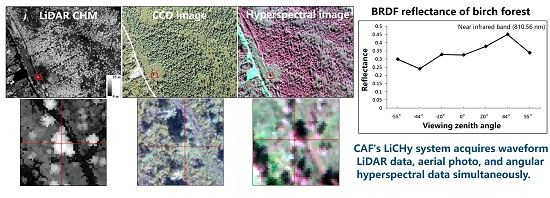
2.2. Airborne Scanning Waveform LiDAR

Full-waveform LiDAR data provide more control to users for vertical information analysis [30] as well as more complete attributes data [31]. The RIEGL LMS-Q680i was selected as laser sensor used in LiCHy. The LMS-Q680i is a full waveform LiDAR system, which gives access to detailed target parameters by digitizing the echo signal online during data acquisition and subsequent off-line waveform analysis. The waveform data recording interval is 1 ns (i.e., about 15 cm per waveform bin). This waveform recording method is especially useful when observing complex vertical distributed targets such as trees. The Multiple-time-around (MTA) technology allows the utilization of target echo signals, which have been detected out of the unambiguity range between two successive laser pulses. This allows the sensor to have a pulse repetition rate of 400 kHz with an effective measurement rate of up to 266 kHz (Riegl GmbH, 2010,) [32]. It is possible to select different pulse repetition rate according to the flight altitude and target reflectance. This system has a wavelength of 1550 nm, with a 0.5 mrad beam divergence and 3 ns pulse length. The maximum average output laser energy is about 40 mW. The scan angle is ±30° perpendicular to the flight direction. The LMS-Q680i uses a rotating polygon mirror with four facets to deflect a laser beam onto the ground. As the mirror moves in a linear angular speed, it results in an approximate even point spacing along the scanning direction.

The scan speed can be set from 10 lines/s to 200 lines/s. Each return from target is time tagged and accurately synchronized with the GPS using a 1 Hz Transistor-Transistor Logic (TTL) pulse. The IGI’s LiteMapper software provides a GUI for laser scanner control and real-time monitoring of laser and flying trajectory data. Ground footprint diameter at 1000 m altitude is about 0.5 m with 1155 m swath width. A point density of up to 4 points/m² can be achieved without considering multiple returns.

2.3. CCD Sensor

A medium-format airborne digital camera system (DigiCAM-60) was selected as the CCD sensor for LiCHy [33]. DigiCAM-60 has 60 million pixels (8956 × 6708), 1.6 s image repetition rate, and 16 bits recording depth. The focal lens is 50 mm. This camera gives a 12 cm spatial resolution with flying altitude of 1000 m.

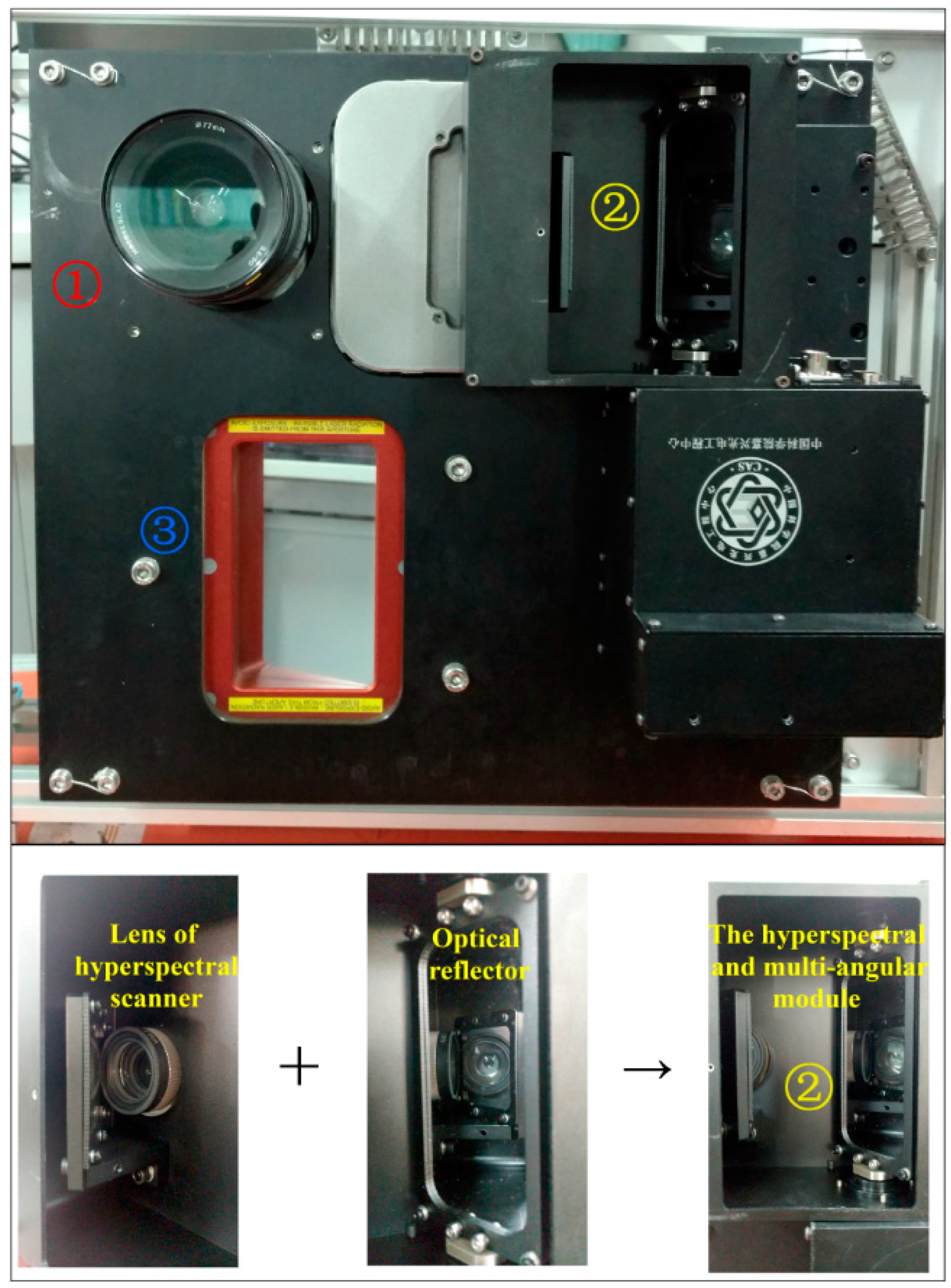
2.4. Hyperspectral Sensor

Hyperspectral sensors are very effective for mapping forest canopy chemical and taxonomic diversity [2]. The AISA Eagle II (Spectral Imaging Ltd., Oulu, Finland) was selected as the hyperspectral sensor for LiCHy system [34]. It is a push broom imaging system, comprising a hyperspectral sensor and a data acquisition unit housed in a rugged control computer. The AISA Eagle II covers the VNIR spectral ranges from 400 nm to 970 nm, with 512 or 1024 bins in spatial direction. The image rate can be up to 160 Hz, the focal length is 18.1 mm, and the field of view (FOV) is 37.7°. It can acquire up to 488 spectral bands at the maximum sample spectral resolution of 1.15 nm. The highest spectral resolution in terms of FWHM is 3.3 nm. Four modes of spectral binning options are provided, which are 1×, 2×, 4× and 8×, with corresponding band numbers of 488, 244, 122 and 60. The mode parameters of spatial and spectral resolution can be modified according to the flight altitude and speed. The maximum frame rate varies from 30 to 160 frames/s with different spectral and spatial resolution configurations. The ground resolution at 1000 m altitude is about 0.68 m with a swath width of 680 m. The instrument provides a radiometric calibration file for each band, which can help users to get the radiance of the target object.

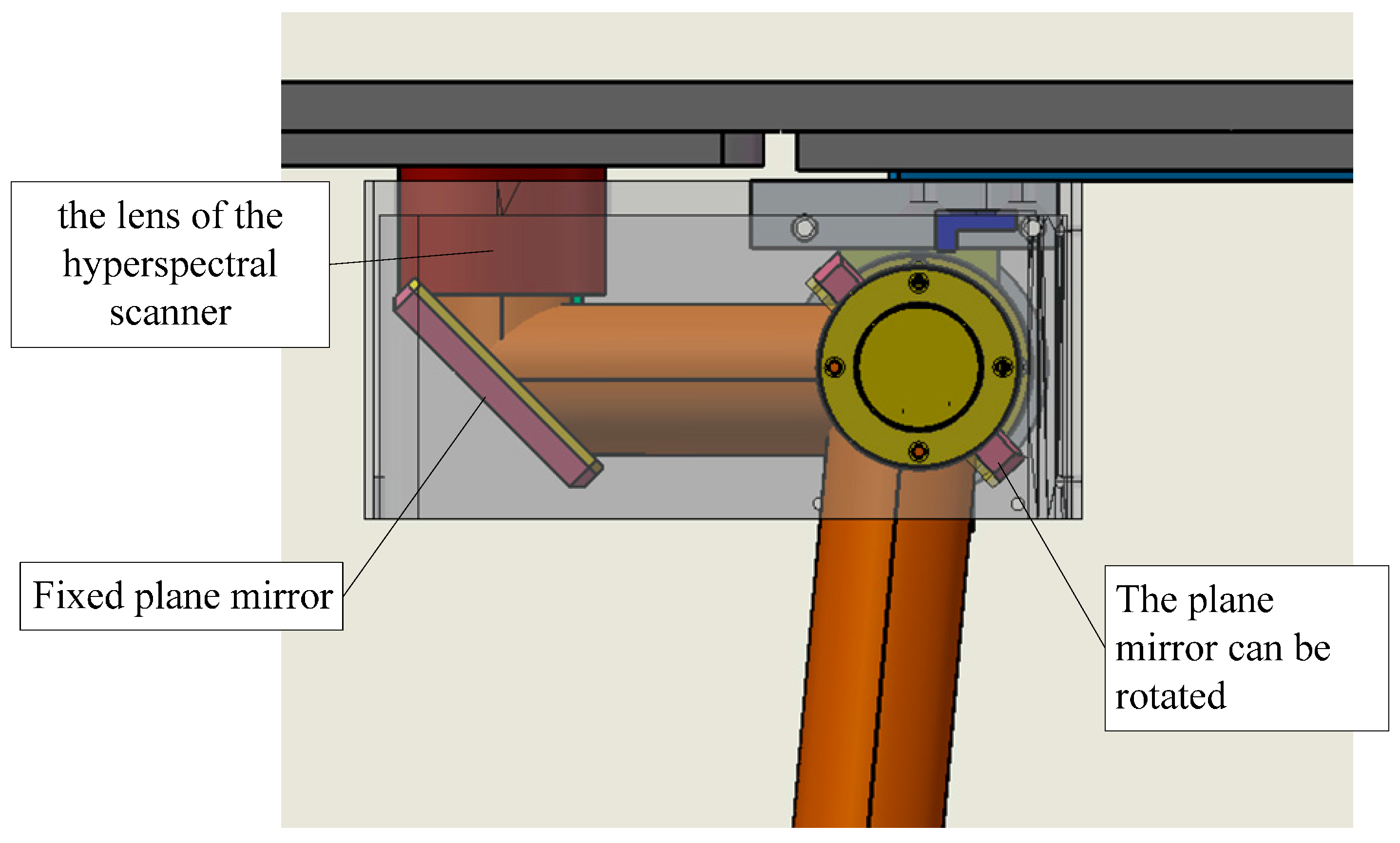
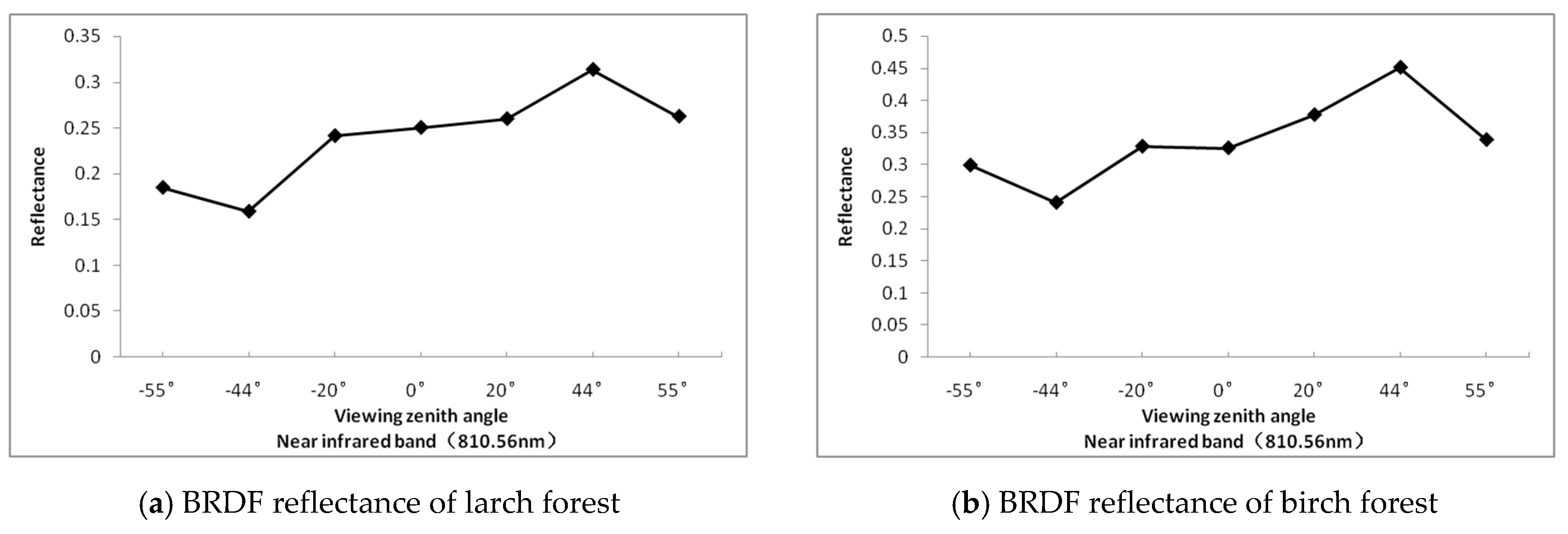
2.5. Multi-Angular Hyperspectral Module (MAM)

The multi-angular hyperspectral module (MAM) is an add-on component to the hyperspectral sensor, which is used to change the optical angle of the hyperspectral sensor, allowing targets to be scanned at multiple angles. The module has two plane mirrors to achieve a variable incidence angle (Figure 1). The first is a fixed plane mirror, which can change the optical direction from vertical to horizontal. The second plane mirror is rotated by an ultrasonic motor. The motor can change the angle of optical direction from 5 to 55 degrees, with a precision of 0.01 degree. The observation angle can be changed in real-time during the flight. This optical device is rigidly attached to the housing framework of the LiCHy system and shares the same power system with the other components. The hyperspectral instrument is installed on the steel plate in the front of the MAM. The MAM was then aligned successively to the plate so that the lens of the hyperspectral scanner and the multi-angle optical system are bound firmly.

As the mirrors change the optical path of light that enters the hyperspectral lens, the geometric model of the scanner is fundamentally distorted. To rebuild the correct geocoding procedure, the new “virtual” optical center of the hyperspectral scanner with respect to the IMU is estimated by considering the position and orientation of deflecting mirrors. The rotation angle of a scanning line is recorded from the readout of controlling interface and used in the georectification post-processing. To guarantee the geometric accuracy of geocoding, a strict geometric boresight flight is needed in the flight campaign to determine the mirror’s rotation error and mounting errors. Then the boresight parameters could be estimated and applied separately to data of each incident angle.

3. LiCHy System Integration

The IMU is set up on the top of laser scanner, which provides the fixed mount relationship between the center of the IMU and the laser scanner. The laser scanner, CCD and hyperspectral sensor are aligned on a single reinforced steel plate. This mount pattern keeps good relative mount relationships with the IMU. Further space is available for another optional sensor integration, such as a thermal camera or a shortwave infrared hyperspectral sensor in addition to ASIA Eagle. Currently, the multi-angular hyperspectral module (MAM) is mounted here.

Figure 2 shows the spatial distribution pattern of the three earth observation sensors. The configuration of the earth observation parts of the integrated system is similar in size as traditional photogrammetry cameras or stabilization platforms, which means the LiCHy system can be mounted easily on general purpose aircrafts with standard photogrammetry hatches. This is helpful for selecting an aircraft available within or near a project area, potentially saving significant time and cost. On the other hand, in this configuration, the three sensors were not along a single optical axis. As the hyperspectral sensor has the narrowest view angle of 37.7°, the three sensors still cover the same overlap area as hyperspectral sensor does (as shown in Figure 3).

The IGI’s Sensor Management Unit (SMU) within the AEROcontrol system was used to control and communicate among GNSS, IMU and the three earth observation sensors, in order to determine the position and status precisely for the data from each sensor. The IGI’s Computer Controlled Navigation System (CCNS) was used to manage flight lines and pilot navigation.

The onboard INS needs an initial alignment before the aircraft moving, in the order of 3–5 min. At the same time, the GNSS receiver can be started and in order to receive the GNSS signals correctly during the whole flight period. The AEROcontrol gives each individual instrument a PPS (pulse per second) cable that synchronizes the time stamps. When the instruments collect data, they store the time tags for every frame or pulse.

4. Sensor Calibration and Data Processing

The data flow of LiCHy airborne observation system is shown in Figure 4. It starts from flight lines planning, mission management and data collection. After on-board data exported to in-house hard drive, we firstly process GNSS and INS data for trajectories information, then process the three observation data from CCD, LiDAR and hyperspectral sensors.

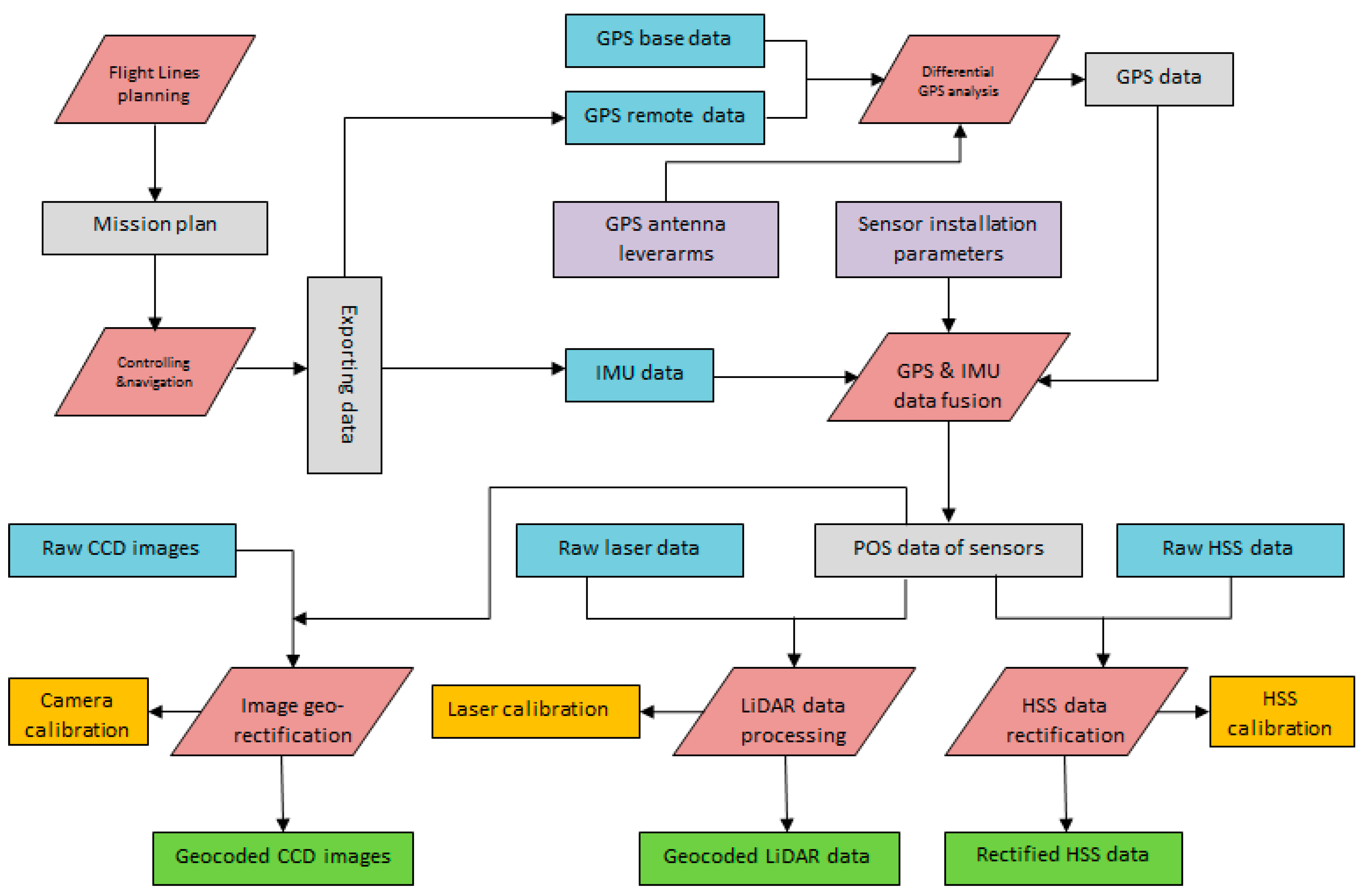
4.1. GNSS and INS Data Processing

The GNSS and INS data are the original reference for the LiCHy system to assign coordinates and orientation to all the sequential observations. The individual GNSS observation records the position of phase center of its antenna during the data acquisition. To achieve a more reliable GNSS solution, in the processing flow, two strategies of data collection are often used, i.e., post-differencing and precise point positioning (PPP). If ground GNSS references (e.g., ground station) are available, the absolute references are used to differentiate the GPS data onboard. Otherwise the precise ephemeris files will be used instead.

The differentiated GPS data and INS data are imported into the post-processing software (AEROoffice, Kreuztal, Germany). A Kalman filter (forward computation and backward computation) is used to produce accurate trajectory files. The post-processed data (positions, velocities and angles) can be output for selected sensors with discrete events (e.g., CCD camera) or continuously operating sensors (e.g., LiDAR and hyperspectral scanner).

4.2. LiDAR Data Processing

The workflow of LiDAR data post-processing is shown in Figure 5. The detailed steps are as follows:

(1)

Full Waveform Decomposition. As LiCHy always enables the continuous collection of full waveform signal, the raw waveform sample data are the first processing object for more advanced LiDAR information, also to reduce the data amount stored by separating the individual pulse returns. Three decomposition methods (i.e., Center Of Gravity estimation, Gaussian Pulse Fitting, and Gaussian Pulse Estimation) are implemented in the processing software of RiProcess [32], all for pulse ranging and extra waveform properties (e.g., pulse width, amplitude).

(2)

Geocoding. As the extracted discrete returns of the first step do not contain geographical properties, it is a prerequisite that all the pulses have to be assigned with correct geolocations. The pulse repeat rate (PRR) of the laser is much higher than the data rate of INS. In this step, the POS data are interpolated to provide position and orientation information for each laser pulses. By establishing the geometric model, all the pulse origins and directional vectors can be recovered with the aid of POS data. The LiDAR range ambiguity is resolved by an advanced processing strategy driven by a prior coarse resolution DEM [35].

(3)

Boresight Calibration. Limited techniques for integrating the laser and INS introduce errors between the axes of the LiDAR and the POS coordinate systems. To correct these misalignments, boresight calibration is needed with well-planned flight lines and careful post-processing. The boresight angles (i.e., roll, pitch and yaw) are estimated by recognizing identical solid targets in overlapping areas of different lines and applied them back to the laser instrument parameters. As the boresight angles directly change the former geocoding results, geocoding process for flight lines will be performed again to achieve better solutions. Normally these two steps need to be looped several times over the data from calibration flight lines before the residual errors of identical targets do not decrease significantly.

4.3. CCD Data Processing

The CCD images in the LiCHy system are stored with a series of stamps in the raw POS data where the exposure signals can also be associated with precise time stamps. The POS records are interpolated to calculate the elements of exterior orientation for each exposure. The CCD lens and mount parameters are usually refined in TerraPhoto software [36]. TerraPhoto was selected because it is specifically designed for handling images taken during laser scanning missions to produce accurate ground models, one of LiCHy’s main objectives. Orthorectified images are then produced as one of the final products of the LiCHy system.

4.4. Hyperspectral Data Processing

Figure 6 shows an overview of the hyperspectral data operational workflow, including radiometric correction and georeference correction.

The raw AISA Eagle hyperspectral images are calibrated and georeferenced using the CaligeoPRO software (SPECIM Spectral Imaging Ltd., Oulu, Finland). The atmospheric and illumination effects were corrected with ATCOR4 software (ReSe Applications Schläpfer, Wil, Switzerland), which is based on the MODTRAN5 code [37], to get surface reflectance products.

Since a small angular error in vertical alignment between the GNSS/INS system and the hyperspectral sensor could cause a significant pointing error over the long distance between the sensor platform and the ground, the GNSS/INS alignment is calibrated and precisely measured with a procedure known as boresight calibration. When the system is installed, re-installed, or moved within the aircraft, small changes in the alignment might occur, which requires a boresight calibration with special configuration of flight lines. At least three overlapping flight lines flown in different directions are needed in order to tie the points selected on overlapping strips. After running the boresight geometric calibration, the adjustment values (including roll, pitch, and yaw) are computed, then these values are used to optimize the hyperspectral images geometrically. To eliminate the GNSS/INS initial errors, a boresight geometric calibration is needed prior to normal flight data processing.

Georectification is of great importance when preprocessing multi-angle hyperspectral images, since the results influence the identification accuracy of same objects from different observation angles. Processing of multi-angle hyperspectral images is similar to nadir observations, with the difference that an off-nadir observation angle has to be applied as the initial pitch angle. After conducting boresight geometric calibration of the overlapping areas, we obtain the updated adjustment parameters including roll, pitch and yaw. Both of the pitched observation angle and boresight parameters were used together to process the rest of images in the CaligeoPro software package [34].

4.5. Data Products Accuracy

The POS data fusion progress is evaluated with the position/velocity differences between INS and GNSS. In most cases, the position difference is less than 1 cm in north, east, and up/down directions. The velocity difference is generally less than 1 m/s according to the POS processing results.

For each flight campaign, a small area with regular ground targets (e.g., urban areas) is selected for a calibration flight. Several flight lines are designed as the ‘‘#’’ shape with intersections and overlapping and flown with lower altitude for all sensors. One more flight line with diagonal direction across ‘‘#’’ shape is also needed for the hyperspectral sensor calibration. The geometrical calibration of the LiDAR is semi automatically performed by detecting plane tie objects and calculating the instrument orientation errors. Crossing lines are also used for the geometric calibration of the hypersectral scanner and the CCD camera.

After applying the appropriate calibration parameters to the whole dataset of a campaign, the matching errors in overlapping regions within a certain sensor product and between different sensor products are then reduced significantly. The matching errors of overlapping scan lines in LiDAR point cloud are generally less than 10 cm both vertically and horizontally at the altitude of 1000 m and can be reduced to less than 5 cm at lower altitudes. The average matching errors between LiDAR, HSS and CCD imagery are generally within 1–2 pixels, mainly dependent on the terrain situation and the calibration quality.

As the geo-location of LiDAR is directly determined by INS and DGPS system, the LiDAR products are used as a reference map for further product analyses. The horizontal accuracy of LiDAR is about 0.5 m and the vertical accuracy is about 0.3 m after comparing with typical observation targets. The consistency of LiDAR and CCD products is within 1 pixel for gentle slope areas and 1–2 pixels for hilly areas. The geo-location accuracy of hyperspectral image is within 2 pixels comparing to LiDAR product for nadir view observations and decreases to 5–7 pixels for large off-nadir observations of 55° with multi-angle modular.

5. Data Collection Using LiCHy System

CAF’s LiCHy (LiDAR, CCD and Hyperspectral) Airborne Observation System is a unique system that permits simultaneous measurements of vegetation vertical structure, horizontal pattern and foliar spectra at very high spatial resolution on a wide range of airborne platforms. The complementary nature of LiCHy sensors makes it valuable for comprehensive forest inventory, forest disturbance monitoring, biodiversity evaluation and carbon accounting. Figure 7 shows sample LiCHy measurements at a temperate forest with high vertical resolution data from full waveform LiDAR, high horizontal resolution images from CCD, and vegetation spectra from the hyperspectral sensor. These three types of data have good geolocation coincidence, a fundamental aspect for further processing like data fusion.

From June 2013 to September 2015, the LiCHy system acquired data over an area of 8000 km² in China (

Table 2. General descriptions of CAF-LiCHy data coverage sites from 2013 to 2015.

No.	Site Name with Central Coordinates	Date, Area and Vegetation Type	Objectives
1	Genhe, Inner Mongolia (121°35′ E, 50°56′ N)	August 2015; 120 km2 Temperate forest	LiDAR and multi-angle hyperspectral fusion
2	Maoershan, Heilongjiang Prov. (127°36′ E, 45°21′ N)	September 2015; 360 km2 Temperate forest	Forest inventory, productivity, carbon accounting
3	Ejina, Gansu Prov. (101°07′ E, 42°0′ N)	July 2014; 220 km2 Dry land forest	Watershed application
4	Beijing (115°58′ E, 40°27′ N)	September 2013; 80 km2 Temperate forest	Urban forestry, biomass
5	Anyang, Henan Prov. (114°20′ E, 36° 7′ N)	June 2013; 50 km2 Temperate forest	System calibration and testify, urban forestry, land cover
6	Yancheng, Jiangsu Prov. (120°49′ E, 32°52′ N)	November 2014; 320 km2 Coastal forest and wetland low vegetation	Wetland and coastal region application, plantation forest, land cover, habitat
7	Huangshan, Anhui Prov. (118°14′ E, 29°32′ N)	September to October 2014; 2900 km2 Subtropical forest	Regional scale forest biomass mapping, biodiversity application, change detection
8	Changshu, Jiangsu Prov. (120°42′ E, 31°40′ N)	August, 2013; 60 km2 Subtropical forest	Forest parameter estimation, fuel mapping
9	Puer, Yunnan Prov. (100°56′ E, 22°44′ N)	December 2013 to April 2014; 4060 km2 Subtropical and tropical forest	Regional scale forest biomass mapping, productivity, biodiversity application

). These sites were ordered from north to south, and the observations covered temperate forest, subtropical forest, tropical forest, coastal forest and dry land forest, providing a comprehensive dataset for data fusion and forest related investigations. The LiCHy system focuses on forest monitoring, but the system can also be effectively used for other vegetation types (e.g., wetland vegetation in site 6, shrubs in sites 3 and 6) and for other remote sensing applications.

The collection of these datasets was driven by some national and provincial scientific projects, and forest institutions and research organizations. The metadata and thematic outputs will be available on the National Forest Scientific Data Platform (http://www.forestdata.cn/). To access and share the original dataset, some signed data sharing agreements are needed according to the Chinese Survey Laws and related regulations.

Figure 8 showed multi-angle hyperspectral data collected in August 2015 in Greater Xing’an Mountains (Genhe site). The view angles include 0°, −20°, −44°, −55°, and 20°, 44°, 55°. These angles covered typical observation angles of multi-angle systems like MISR and CHRIS/PROBA [26,28]. The hot-spot and cold-spot angles were calculated according to the geo-location and observation date.

The BRDF curve showed that multi-angle data characterize well the directional reflectance information of vegetation (Figure 9). The hot-spot (i.e., highest reflectance value) was located at around 44° and the cold-spot (i.e., lowest reflectance value) was found at around −44° with lowest reflectance value. This is consistent with the sun elevation angle for the Genhe test site in the Greater Xing’an Mountains (site 1 in Table 2), which varied among 42°~46° during the flight period.

The data collected by the LiCHy system covered typical forests in China. These data will support the quantification analysis of forest parameters and the investigation of a satellite concept of LiDAR and passive optical sensor configuration.

6. Potential Forest Applications of Data from LiCHy System

The multiple types of observation data from LiCHy system provide extended potential for forest various applications. Hudak et al. (2009) reviewed LiDAR applications for natural resource management [38]. With increasing amounts and improved data quality, acquired simultaneously, LiCHy expands these possibilities.

Table 3. Potential forest applications of data from LiCHy sensors.

Sensor	Data Products	Potential Applications
Waveform LiDAR	Waveform and point cloud	Topography, hydrology, watershed
	DTM	Forest height, density, volume, biomass estimation
	DSM
	CHM
	LiDAR metrics (height, density, structural)	Structural estimation, biodiversity
CCD camera	Aerial photo	Forest distribution, gap
	Texture	Horizontal information
Hyperspectral sensor	Reflectance	Forest composition
	Vegetation indices	Health, vigor
	Species	Biodiversity
	Pigments
With Multi-angle	BRDF	Structural estimation, biodiversity
Modular	Structural indices	Forest height, volume, biomass
Fusion	Improved species classification with structural information integrated	Carbon accounting
	Improved forest parameter estimation with species stratification	Forest inventory and management
	Forest management unit segmentation	Biodiversity, ecosystem services
	Data extrapolation among sensors	Satellite mission concept development

lists a number of potential forest-related applications of LiCHy data. The three different types of earth observation sensors can be used separately, providing high quality waveform LiDAR data, high spatial resolution aerial photo, and multi-angle hyperspectral data. Besides all these traditional applications, the collection of simultaneous data provides a unique opportunity for novel data fusion techniques, with these multi-type data fusion providing better estimation accuracies and further potential applications. The vertical information from waveform LiDAR will improve our capabilities to accurately classify hyperspectral data, especially for more complex, multi-level forest structures. In addition, with the support of canopy height models (CHMs) from LiDAR data, hyperspectral data could be used to identify vegetation types among canopy gaps. As demonstrated by Tompalski et al. (2014), different species impact stand volume estimations dramatically. Improved forest species or species group classification can be used to build stratified model for LiDAR metrics, of crucial importance for accurate estimations of forest volume, biomass and carbon accounting [39].

Forest parameters from LiDAR data are widely used as reference data [7,12], but the extrapolation of these limited LiDAR estimates to a broad regions or continuous mapping is typically based on the currently available satellite data like MODIS or MISR [26,40]. Multi-angular hyperspectral observations can help validate these satellite products while being beneficial for future joint LiDAR and optical sensor satellite mission for forest monitoring purposes [25,27,41].

7. Conclusions

We presented the CAF’s multi-sensor airborne system LiCHy, which has unique observation capability of simultaneous waveform LiDAR, aerial photography, and spectra from different viewing angles. At the time of the writing, the CAF’s LiCHy system has collected more than 8000 km² data over typical forests across China. These simultaneous measurements of vegetation vertical structure, horizontal pattern, and foliar spectra will be integrated to further explore well-established applications of remote sensing in forestry, such as forest inventory, forest disturbance monitoring, and biodiversity evaluation, as well as to investigate the capabilities of novel approaches based on simultaneous LiDAR and optical remote sensing applications in forest management, the development of similar satellite configuration, and forest carbon accounting.

References

1. Wulder, M.A.; Bater, C.W.; Coops, N.C.; Hilker, T.; White, J.C. The role of LiDAR in sustainable forest management. For. Chron. 2008, 84, 807–826. [Google Scholar] [CrossRef]
2. Asner, G.P.; Martin, R.E. Airborne spectranomics: Mapping canopy chemical and taxonomic diversity in tropical forests. Front. Ecol. Environ. 2009, 7, 269–276. [Google Scholar] [CrossRef]
3. Riedler, B.; Pernkopf, L.; Strasser, T.; Lang, S.; Smith, G. A composite indicator for assessing habitat quality of riparian forests derived from Earth observation data. Int. J. Appl. Earth Obs. Geoinform. 2015, 37, 114–123. [Google Scholar] [CrossRef]
4. Ip, A.; El-Sheimy, N.; Mostafa, M. Performance analysis of integrated sensor orientation. Photogramm. Eng. Remote Sens. 2007, 73, 89–97. [Google Scholar] [CrossRef]
5. Næsset, E.; Gobakken, T.; Holmgren, J.; Hyyppä, H.; Hyyppä, J.; Maltamo, M.; Nilsson, M.; Olsson, H.; Persson, Å.; Söderman, U. Laser scanning of forest resources: The Nordic experience. Scand. J. For. Res. 2004, 19, 482–499. [Google Scholar] [CrossRef]
6. Vierling, K.T.; Vierling, L.A.; Gould, W.A.; Martinuzzi, S.; Clawges, R.M. Lidar: Shedding new light on habitat characterization and modeling. Front. Ecol. Environ. 2008, 6, 90–98. [Google Scholar] [CrossRef]
7. Wulder, M.A.; White, J.C.; Bater, C.W.; Coops, N.C.; Hopkinson, C.; Chen, G. Lidar plots—A new large-area data collection option: Context, concepts, and case study. Can. J. Remote Sens. 2012, 38, 600–618. [Google Scholar] [CrossRef]
8. Zhao, D.; Pang, Y.; Li, Z.; Liu, L. Isolating individual trees in a closed coniferous forest using small footprint lidar data. Int. J. Remote Sens. 2014, 35, 7199–7218. [Google Scholar] [CrossRef]
9. Duncanson, L.I.; Dubayah, R.O.; Cook, B.D.; Rosette, J.; Parker, G. The importance of spatial detail: Assessing the utility of individual crown information and scaling approaches for lidar-based biomass density estimation. Remote Sens. Environ. 2015, 168, 102–112. [Google Scholar] [CrossRef]
10. Hansen, E.H.; Gobakken, T.; Bollandsås, O.M.; Zahabu, E.; Næsset, E. Modeling aboveground biomass in dense tropical submontane rainforest using airborne laser scanner data. Remote Sens. 2015, 7, 788–807. [Google Scholar] [CrossRef] [Green Version]
11. Zolkos, S.G.; Goetz, S.J.; Dubayah, R. A meta-analysis of terrestrial aboveground biomass estimation using lidar remote sensing. Remote Sens. Environ. 2013, 128, 289–298. [Google Scholar] [CrossRef]
12. Asner, G.P.; Knapp, D.E.; Martin, R.E.; Tupayachi, R.; Anderson, C.B.; Mascaro, J.; Sinca, F.; Chadwick, K.D.; Higgins, M.; Farfan, W.; et al. Targeted carbon conservation at national scales with high-resolution monitoring. Proc. Natl. Acad. Sci. USA 2014, 111, E5016–E5022. [Google Scholar] [CrossRef] [PubMed]
13. Hilker, T.; Coops, N.C.; Nesic, Z.; Wulder, M.A.; Brown, M.; Black, A.T. Instrumentation and approach for unattended year round tower based measurements of spectral reflectance. Comput. Electron. Agric. 2007, 56, 72–84. [Google Scholar] [CrossRef]
14. Tortini, R.; Hilker, T.; Coops, N.C.; Nesic, Z. Technological advancement in tower-based canopy reflectance monitoring: The AMSPEC-III system. Sensors 2015, 15, 32020–32030. [Google Scholar] [CrossRef] [PubMed]
15. Simic, A.; Chen, J.M.; Freemantle, J.; Miller, J.R.; Pisek, J. Improving clumping and LAI algorithms based on multi-angle airborne imagery and ground measurements. IEEE Trans. Geosci. Remote Sens. 2010, 48, 1742–1759. [Google Scholar] [CrossRef]
16. Koetz, B.; Morsdorf, F.; Van der Linden, S.; Curt, T.; Allgöwer, B. Multi-source land cover classification for forest fire management based on imaging spectrometry and LiDAR data. For. Ecol. Manag. 2008, 256, 263–271. [Google Scholar] [CrossRef]
17. Geerling, G.W.; Abrador-Garcia, M.; Clevers, J.G.P.W.; Ragas, A.M.J.; Smits, A.J.M. Classification of floodplain vegetation by data fusion of spectral (CASI) and LiDAR data. Int. J. Remote Sens. 2007, 28, 4263–4284. [Google Scholar] [CrossRef]
18. Liu, L.J.; Pang, Y.; Fan, W.Y.; Li, Z.Y.; Zhang, D.R.; Li, M.Z. Fused airborne LiDAR and hyperspectral data for tree species identification in a natural temperate forest. J. Remote Sens. 2013, 17, 679–695. [Google Scholar]
19. Pang, Y.; Tan, B.; Solberg, S.; Li, Z. Forest LAI estimation comparison using LiDAR and hyperspectral data in boreal and temperate forests. SPIE Opt. Eng. Appl. 2009, 7454. [Google Scholar] [CrossRef]
20. Asner, G.P.; Knapp, D.E.; Kennedy-Bowdoin, T.; Jones, M.O.; Martin, R.E.; Boardman, J.; Field, C.B. Carnegie airborne observatory: In-flight fusion of hyperspectral imaging and waveform light detection and ranging for three-dimensional studies of ecosystems. J. Appl. Remote Sens. 2007, 1, 013536. [Google Scholar] [CrossRef]
21. Kampe, T.U.; Johnson, B.R.; Kuester, M.; Keller, M. NEON: The first continental-scale ecological observatory with airborne remote sensing of vegetation canopy biochemistry and structure. J. Appl. Remote Sens. 2010, 4, 043510. [Google Scholar] [CrossRef]
22. National Ecological Observatory Network (NEON). Available online: http://www.neoninc.org/science-design/collection-methods/airborne-remote-sensing (accessed on 12 October 2015).
23. Asner, G.P.; Knapp, D.E.; Boardman, J.; Green, R.O.; Kennedy-Bowdoin, T.; Eastwood, M.; Martin, R.E.; Anderson, C.; Field, C.B. Carnegie Airborne Observatory-2: Increasing science data dimensionality via high-fidelity multi-sensor fusion. Remote Sens. Environ. 2012, 124, 454–465. [Google Scholar] [CrossRef]
24. Cook, B.D.; Nelson, R.F.; Middleton, E.M.; Morton, D.C.; McCorkel, J.T.; Masek, J.G.; Ranson, K.J.; Ly, V.; Montesano, P.M. NASA Goddard’s LiDAR, hyperspectral and thermal (G-LiHT) airborne imager. Remote Sens. 2013, 5, 4045–4066. [Google Scholar] [CrossRef]
25. Hese, S.; Lucht, W.; Schmullius, C.; Barnsley, M.; Dubayah, R.; Knorr, D.; Neumann, K.; Riedel, T.; Schröter, K. Global biomass mapping for an improved understanding of the CO 2 balance—The Earth observation mission Carbon-3D. Remote Sens. Environ. 2005, 94, 94–104. [Google Scholar] [CrossRef]
26. Chopping, M.; Moisen, G.G.; Su, L.; Laliberte, A.; Rango, A.; Martonchik, J.V.; Peters, D.P. Large area mapping of southwestern forest crown cover, canopy height and biomass using the NASA Multiangle Imaging Spectro-Radiometer. Remote Sens. Environ. 2008, 112, 2051–2063. [Google Scholar] [CrossRef]
27. Chopping, M.; Nolin, A.W.; Moisen, G.G.; Martonchik, J.V.; Bull, M. Forest canopy height from Multiangle Imaging Spectro-Radiometer (MISR) assessed with high resolution discrete return lidar. Remote Sens. Environ. 2009, 113, 2172–2185. [Google Scholar] [CrossRef]
28. Schlerf, M.; Atzberger, C. Vegetation structure retrieval in beech and spruce forests using spectrodirectional satellite data. IEEE J. Sel. Top. Appl. Earth Obs. Remote Sens. 2012, 5, 8–17. [Google Scholar] [CrossRef]
29. AEROcontrol & AEROoffice. Available online: http://www.igi.eu/aerocontrol.html (accessed on 11 October 2015).
30. Mallet, C.; Bretar, F. Full-waveform topographic LiDAR: State-of-the-art. ISPRS J. Photogramm. Remote Sens. 2009, 64, 1–16. [Google Scholar] [CrossRef]
31. Anderson, K.; Hancock, S.; Disney, M.; Gaston, K.J. Is waveform worth it? A comparison of LiDAR approaches for vegetation and landscape characterization. Remote Sens. Ecol. Conserv. 2015, 2, 5–15. [Google Scholar] [CrossRef]
32. RIEGL LMS-Q680i. Available online: http://www.riegl.com/products/airborne-scanning/produktdetail/product/scanner/23/ (accessed on 9 October 2015).
33. DigiCAM-Digital Aerial Camera. Available online: http://www.igi.eu/digicam.html (accessed on 9 October 2015).
34. AISA Eagle II. Available online: http://www.specim.fi/index.php/products/airborne (accessed on 9 October 2015).
35. Lu, H.; Pang, Y.; Li, Z.; Chen, B. An automatic range ambiguity solution in high-repetition-rate airborne laser scanner using priori terrain prediction. IEEE Geosci. Remote Sens. Lett. 2015, 12, 2232–2236. [Google Scholar] [CrossRef]
36. Terrasolid Ltd., 2015. TerraPhoto User’s Guide. Available online: http://www.terrasolid.com/download/tphoto.pdf (accessed on 9 October 2015).
37. Richter, R.; Schläpfer, D. Atmospheric/Topographic Correction for Airborne Imagery. ATCOR-4 User Guide Version 7.0.3; ReSe Applications Schläpfer: Wil SG, Switzerland, 2016. [Google Scholar]
38. Hudak, A.T.; Evans, J.S.; Stuart Smith, A.M. LiDAR utility for natural resource managers. Remote Sens. 2009, 1, 934–951. [Google Scholar] [CrossRef]
39. Tompalski, P.; Coops, N.C.; White, J.C.; Wulder, M.A. Simulating the impacts of error in species and height upon tree volume derived from airborne laser scanning data. For. Ecol. Manag. 2014, 327, 167–177. [Google Scholar] [CrossRef]
40. Simard, M.; Pinto, N.; Fisher, J.B.; Baccini, A. Mapping forest canopy height globally with spaceborne lidar. J. Geophys. Res. Biogeosci. 2011, 116. [Google Scholar] [CrossRef]
41. Lefsky, M.A.; Ramond, T.; Weimer, C.S. Alternate spatial sampling approaches for ecosystem structure inventory using spaceborne lidar. Remote Sens. Environ. 2011, 115, 1361–1368. [Google Scholar] [CrossRef]
Figure 1. The optical structural design map of the multi-angular hyperspectral module (MAM).
Remotesensing 08 00398 g001
Figure 2. Layout of lenses of different sensors. ① lens of CCD camera and ② lens of hyperspectral sensor and multi-angular module. ③ reflecting mirror of laser scanner.
Remotesensing 08 00398 g002
Figure 3. Swath angles of different sensors in LiCHy airborne observation system. The observation angle of hyperspectral sensor changes with MAM module.
Remotesensing 08 00398 g003
Figure 4. The data flow of LiCHy airborne observation system.
Remotesensing 08 00398 g004
Figure 5. The workflow of waveform LiDAR data processing.
Remotesensing 08 00398 g005
Figure 6. The workflow of hyperspectral data processing.
Remotesensing 08 00398 g006
Figure 7. Coincident acquisition of LiDAR, CCD, and multi-angle hyperspectral data with LiCHy system in a temperate forest (29 August 2015; 50.931° N, 121.503° E). The top images in the left column are Canopy Height Model (CHM) from LiDAR data, CCD image and hyperspectral image of the same ground target. The middle column shows the enlarged view of the left pictures. The right column shows the side view of point cloud data from single tree, waveform of a single laser pulse and the spectrum of typical targets from hyperspectral data. The bottom images are multi-angle hyperspectral data for viewing zenith angle (VZA) of ±44°, and the derived Normalized Difference between Hotspot and Darkspot (NDHD) map using band of 849.30 nm. The spatial resolutions of CHM data, CCD data and hyperspectral data (VZA = 0°) are 0.5 m, 0.8 m and 0.2 m, respectively. The central wavelengths of displayed hyperspectral image for red, green and blue bands are 849.30, 694.91 and 543.72 nm.
Remotesensing 08 00398 g007
Figure 8. Multi-angle hyperspectral data from CAF-LiCHy AOP system in Greater Xing’an Mountains. The RGB false color channels are 858.99 nm, 647.19 nm, 553.02 nm respectively. The view angles include 0°, −20°, −44°, −55°, and 20°, 44°, 55°.
Remotesensing 08 00398 g008
Figure 9. BRDF reflectance of typical forest types (a,b) in the Greater Xing’an Mountains, Northeast China.
Remotesensing 08 00398 g009