Article

Examining Spectral Reflectance Saturation in Landsat Imagery and Corresponding Solutions to Improve Forest Aboveground Biomass Estimation

1
Key Laboratory of Carbon Cycling in Forest Ecosystems and Carbon Sequestration of Zhejiang Province, School of Environmental & Resource Sciences, Zhejiang Agriculture and Forestry University, Lin’an 311300, China
2
Center for Global Change and Earth Observations, Michigan State University, East Lansing, MI 48823, USA
3
Department of Geography, Southern Illinois University Carbondale, Carbondale, IL 62901, USA
4
Zhejiang Forestry Academy, Hangzhou 310023, China
5
School of Forestry and Biotechnology, Zhejiang Agriculture and Forestry University, Lin’an 311300, China
*
Author to whom correspondence should be addressed.
Remote Sens. 2016, 8(6), 469; https://doi.org/10.3390/rs8060469
Submission received: 3 March 2016 / Revised: 18 May 2016 / Accepted: 30 May 2016 / Published: 2 June 2016
(This article belongs to the Special Issue Digital Forest Resource Monitoring and Uncertainty Analysis)

Abstract

:
The data saturation problem in Landsat imagery is well recognized and is regarded as an important factor resulting in inaccurate forest aboveground biomass (AGB) estimation. However, no study has examined the saturation values for different vegetation types such as coniferous and broadleaf forests. The objective of this study is to estimate the saturation values in Landsat imagery for different vegetation types in a subtropical region and to explore approaches to improving forest AGB estimation. Landsat Thematic Mapper imagery, digital elevation model data, and field measurements in Zhejiang province of Eastern China were used. Correlation analysis and scatterplots were first used to examine specific spectral bands and their relationships with AGB. A spherical model was then used to quantitatively estimate the saturation value of AGB for each vegetation type. A stratification of vegetation types and/or slope aspects was used to determine the potential to improve AGB estimation performance by developing a specific AGB estimation model for each category. Stepwise regression analysis based on Landsat spectral signatures and textures using grey-level co-occurrence matrix (GLCM) was used to develop AGB estimation models for different scenarios: non-stratification, stratification based on either vegetation types, slope aspects, or the combination of vegetation types and slope aspects. The results indicate that pine forest and mixed forest have the highest AGB saturation values (159 and 152 Mg/ha, respectively), Chinese fir and broadleaf forest have lower saturation values (143 and 123 Mg/ha, respectively), and bamboo forest and shrub have the lowest saturation values (75 and 55 Mg/ha, respectively). The stratification based on either vegetation types or slope aspects provided smaller root mean squared errors (RMSEs) than non-stratification. The AGB estimation models based on stratification of both vegetation types and slope aspects provided the most accurate estimation with the smallest RMSE of 24.5 Mg/ha. Relatively low AGB (e.g., less than 40 Mg/ha) sites resulted in overestimation and higher AGB (e.g., greater than 140 Mg/ha) sites resulted in underestimation. The smallest RMSE was obtained when AGB was 80–120 Mg/ha. This research indicates the importance of stratification in mitigating the data saturation problem, thus improving AGB estimation.

Graphical Abstract

1. Introduction

Forests taking carbon dioxide from the atmosphere and accumulating biomass through photosynthesis are an important carbon sink of terrestrial ecosystems. Estimating and mapping forest biomass/carbon stocks become essential for greenhouse gas inventories, global carbon cycle, and climate change modeling [1,2,3]. Various methods such as process models and remote sensing-based approaches have been developed and used [4,5,6,7]. The process models-based methods do not generate spatially explicit predictions and often lead to a large amount of uncertainty for specific sites, partly because too many variables and input parameters are required to run the models and partly because different source data such as climate and soil data have very coarse spatial resolutions [8,9,10]. In contrast, remote sensing-based approaches have become popular due to their unique characteristics in data collection and presentation; that is, multitemporal remote sensing images not only reveal spatial variability, spatial distributions, and patterns of forests but also provide the potential to estimate their changes over time [4,5,6,7]. A large number of research papers on biomass estimation using remote sensing data have been published in the past three decades, as summarized in previous literature review papers (e.g., [4,6,11,12,13,14,15,16,17]).
Various remotely sensed images from optical sensors and radar and lidar systems have been utilized to estimate and map forest biomass/carbon by combining with ground sample plot data [5,6,11,12,13,14,15]. The optical imagery-based technologies are commonly used for biomass estimation due to high correlations between spectral bands and biomass [4,6,17,18,19,20,21,22,23,24,25,26,27,28]. In particular, Landsat images have been the most widely used for forest aboveground biomass (AGB) estimation in the past three decades [5,6,20,24,26,28,29,30,31,32,33,34,35,36], mainly because they are freely downloadable, have a long history, and have medium spatial resolution. The studies deal with different climate zones and forest ecosystems, from tropical to subtropical, temperate, and boreal forests [4,5,6,7,12,13,14,15,20,28,32,37,38,39,40,41,42,43]. However, one common problem is the data saturation in Landsat imagery; that is, spectral reflectance values are not sensitive to the change in biomass of dense and multilayer canopy forests, which results in low accuracy of AGB estimation, especially when AGB is high, such as greater than 130 Mg/ha [5,6,29]. Although this problem has been recognized for a long time, studies have rarely investigated the saturation values of forest AGB for various forest types. A major challenge is the difficulty in collecting sufficient numbers of sample plots for different vegetation types.
Many factors influence the data saturation of Landsat imagery [5,6,44,45,46,47,48]. The limitation of remote sensing data themselves in spectral, spatial, and radiometric resolutions may result in different saturation values of AGB. Data saturation varies depending on vegetation types because of the various capabilities of their surface reflectance in distinguishing vegetation characteristics, including tree species and forest stand structures [6,30]. Moreover, topographic features also affect the data saturation values of forest AGB due to the fact that elevation, slope, and aspect may affect the distribution and composition of tree species, as well as vegetation growth rates and, thus, spectral reflectance. Various methods have been explored to reduce the impacts of data saturation in Landsat imagery on AGB estimation accuracy (see the review paper by Lu et al. [6]). Vegetation indices and textures are often used [21,25,26,27,49,50,51,52,53]. In the moist tropical region of the Brazilian Amazon, Lu et al. [51] compared different vegetation indices—e.g., normalized difference vegetation index (NDVI), perpendicular vegetation index (PVI), soil adjusted vegetation index (SAVI)—from Landsat Thematic Mapper (TM) imagery and found that the vegetation indices including shortwave infrared spectral bands (SWIR) have higher correlation with AGB than others when the forest stand structure is complex, but the vegetation indices including near-infrared wavelength (NIR) improved correlations with AGB in relatively simple forest stand structures. However, high correlation between vegetation indices or spectral bands makes these variables less important in AGB modeling [6,31]. Time series of Landsat imagery is another method to increase AGB estimation accuracy and reduce saturation effects compared to use of a single NDVI [20,34,48].
The heterogeneity of forest stand structures may be the major reason for data saturation. Lu and Batistella [52] examined the relationships between AGB and grey-level co-occurrence matrix-based (GLCM) textural images from Landsat TM imagery in the Brazilian Amazon and found that textural images were especially useful for primary forest AGB estimation due to its complex forest stand structures. Incorporation of textures into spectral responses has proven useful in improving AGB estimation performance because textures can reduce the impacts of heterogeneity [30]. Nichol and Sarker [49] combined spectral variables from the images of two sensors (i.e., advanced visible and NIR radiometer types—AVNIR-2 and SPOT-5) and ratios of texture parameters from the image bands to explore methods for reducing the impacts of data saturation of optical imagery on AGB estimation accuracy. Their study area was located in the Hong Kong Special Administrative Region that lies on the southeast coast of China, just south of the Tropic of Cancer. Their results showed that using the ratios of texture parameters of both sensors together produced higher agreement between observed and estimated forest AGB values than utilizing the texture parameters or ratios of image bands from one sensor alone. They also suggested that the obtained maximum estimate was 500 t/ha, much higher than the saturation levels in other studies using optical sensors [6,31,44]. Other studies also indicated the importance of combining spectral responses and textures from optical or radar data in improving AGB estimation [21,25,26,27,53].
The existing and limited studies on mitigating the impacts of data saturation from optical images on AGB estimation focus mainly on how to extract and use vegetation indices and texture parameters [6,21,26,27,30]. There have been no published reports on how to model the relationships of forest biomass/carbon with spectral variables from remotely sensed images under different classification scenarios by taking into account the heterogeneity of forest stand structures due to tree species composition, tree ages, and topographic features (e.g., slope and aspect). An exception is that a study by Sanga-Ngoie et al. [54] in forest biomass/carbon estimation in Japan using NDVI from Landsat imagery showed that, in addition to forest types, taking tree ages into account could result in considerable improvement of the estimation. This study implied that the combinations of spatial modeling and forest classification by tree species composition, age, and topographic features may allow for a reduction of the data saturation. Therefore, this research aims at estimating the data saturation values in Landsat imagery for different vegetation types and exploring approaches to improving forest AGB estimation by conducting stratification of vegetation types or/and slope aspects in a subtropical region of Zhejiang Province, China.

2. Study Area and Materials

2.1. Description of the Study Area

The study area is located in Zhejiang province of Eastern China, neighboring Fujian, Anhui Jiangxi, and Jiangsu provinces, and Shanghai (Figure 1). Zhejiang has an area of 101,800 km2 and a population of 55 million [55]. This province has a subtropical moist monsoon climate, with annual temperature of 15~18 °C and the highest temperature in July or August, and annual precipitation of 980~2000 mm. Zhejiang has a varying topography, with montane regions in the west and south, hilly areas in the central part, and flat terrain in the northeast. Montane and hilly regions account for approximately 70% of the total area in this province, plains and basins cover 23%, and rivers and lakes occupy approximately 6% [56].
Zhejiang is characterized by rich vegetation types with typical subtropical evergreen broadleaf forests. The dominant vegetation types include coniferous forests (e.g., pine plantations, Chinese fir plantations), evergreen broadleaf forests, mixed needle and broadleaf forests, and bamboo forests. The forests occupy an area of 5,844,200 ha with a bamboo forest area of 782,900 ha. Forest canopy cover was 60.8% [57]. Young and middle-age forests dominate the forested lands. Zhejiang is one of the provinces that have the highest forest canopy cover percentages in China and, therefore, accurately estimating its forest biomass/carbon is necessary. This study area occupies most of the province, covering different terrains from mountainous regions in the south and west to flat terrains in the northeast (Figure 1).

2.2. Collection of Sample Plot Data and Calculation of Forest Aboveground Biomass

A total of 802 sample plots in the study area were inventoried in 2010 and 2011. These plots were systematically allocated on a previous spatial distribution map of forest types. The plots had a size of 20 m × 20 m. Within each plot, the diameter at breast height (DBH) of greater than 5 cm for each tree was measured. Three subplots of 2 m × 2 m were nested within each plot for measuring seedling and grass biomass [58]. A detailed description of forest inventory and AGB calculation through allometric equations by tree species or species group is provided in Yuan et al. [59]. The sample plots were allocated in different vegetation types, including pine, Chinese fir (hereafter fir), broadleaf forest, mixed forest, bamboo, and shrub. Table 1 summarizes the statistical features of the sample plots for the vegetation types. The sample plots had a mean AGB of 89.61 Mg/ha with a standard deviation of 38.39 Mg/ha and a coefficient of variation of 42.84%. The mixed forests had the highest mean AGB but the smallest coefficient of variation. Fir plantations had the largest standard deviation and pine forests had the largest maximum AGB values. Shrubs had the smallest mean AGB and standard deviation values but had the highest coefficient of variation.
The plot AGB values were divided into five groups with an interval of 40 Mg/ha, and the numbers of sample plots for the AGB groups are summarized in Table 2. Most sample plots fell in the three middle groups, that is, within the range of 40–160 Mg/ha. Of the 802 sample plots, 589 (approximately 75% of all plots) were randomly selected and used for developing AGB estimation models and the remaining 213 plots (25%) were utilized for evaluating AGB estimates. The sample plots are summarized in Table 3 according to different vegetation types and slope aspects. The slope aspects were divided into four groups: semi-sunny (45–135 degree), sunny (135–225 degree), semi-shady (225–315 degree), and shady (315–45 degree) based on the ASTER GDEM data. The number of sample plots for each vegetation type and for each slope aspect is also summarized in Table 3, according to modeling and evaluation purposes.

2.3. Collection of Remote Sensing and DEM Data and Preprocessing

Two Landsat 5 TM images (path/rows: 119/39 and 119/40) with L1T (systematic precision and terrain corrected) products, acquired on 24 May 2010, were used in this research. The images have six spectral bands consisting of three visible bands, one NIR band, and two SWIR bands. Both images have a Universal Transverse Mercator coordinate system with zone 50 north and were mosaicked into one image. The dark object subtraction approach [45] was used to conduct atmospheric calibration so that the surface reflectance values ranged from 0 to 1. The ASTER GDEM data with spatial resolution of 30 m × 30 m at the same coordinate system as the TM image were used to conduct topographic correction for the Landsat 5 TM image using the C-correction approach [46,60].

2.4. Preparation of Vegetation Classification Data

Table 4 provides the definitions of each vegetation type based in the forest inventory data. In order to conduct supervised classification, selection of sufficient numbers of representative sample plots is critical. In this research, three datasets—field survey data collected in 2014, forest inventory plot data collected in 2010 and 2011, and RapidEye images acquired in 2011—were used to select sample plots for this classification. Separability analysis of the vegetation classes was conducted using the transformed divergence algorithm [47]. Refinement of training sample plots for each class was conducted based on the analysis of spectral curves of sample plots for each vegetation type. Approximately 50% of the sample plots were used as training samples and the remaining sample plots were used for accuracy assessment of classification. Figure 2 illustrates the framework of mapping vegetation distribution using Landsat 5 TM imagery in this study area, including (1) preparation of training and test sample plots; (2) image preprocessing and extraction of non-vegetation classes (e.g., impervious surface area (ISA) and water bodies); (3) extraction of spectral signatures for vegetation types; (4) vegetation classification using maximum likelihood classifier (MLC); (5) evaluation of classification result.
Previous research has indicated that MLC is one of the best classification approaches, especially when a sufficient number of representative sample plots are available and spectral signatures are used [47,61]. Therefore, this research used MLC for vegetation classification after ISA and water bodies were masked out. Since ISA has a wide variation in spectral signatures, resulting in spectral confusion between ISA and other land covers such as bare soils in agricultural lands, water and wetlands, and shadows [62], ISA is first extracted from Landsat multispectral imagery using a hybrid approach consisting of linear spectral mixture analysis (LSMA), decision tree classifier, and unsupervised classifier (see details in Li et al. [63]). Water was extracted using the threshold-based approach from the modified normalized difference water index (MNDWI) [64]. The spectral imagery after masking out ISA and water classes was used to conduct vegetation classification using MLC.
Figure 3 illustrates the classification result. Broadleaf forests dominated the western part of the study area and were scattered in the central, southern, and southeastern parts. Pine, fir, and mixed forests were mainly distributed in the southern and southeastern parts. Farmlands and built-up areas were mainly distributed in the northern and northeastern flat area and the belt from the central to the southwestern parts called Jin-Ju basin. This vegetation classification result was used in the mapping of AGB distribution through the established AGB estimation models based on the stratification of vegetation types.
Based on test sample plots, the accuracy assessment result using the error matrix approach is summarized in Table 5, in which overall classification accuracy, kappa coefficient, producer’s accuracy (PA) and user’s accuracy (UA) were also calculated [65]. An overall accuracy of 78.4% and kappa coefficient value of 0.74 were obtained. Bamboo forest had high UA and PA and shrub had low accuracies. Mixed forest is a complex type that can be confused with pine, fir, and broadleaf forests, resulting in low PA.

3. Methods

3.1. Estimation of AGB Saturation Values

In Landsat TM imagery, different vegetation types show their own AGB saturation values due to their different forest stand structures and species compositions. The spectral surface reflectance values of sample plots were extracted from each Landsat spectral band. Pearson product-moment correlation coefficient between plot AGB and each spectral band was analyzed. The image band with the highest correlation coefficient was selected to examine the data saturation value of AGB for each vegetation type. This analysis was initially conducted through analysis of scatterplots; that is, the values of spectral reflectance (Y axis) with the highest correlation coefficient were graphed against the values of AGB at plot level (X axis). A semi-variogram-based approach that is used to model spatial autocorrelation of a variable of interest in geostatistics was utilized to fit the relationship between vegetation AGB and the selected spectral band. Here, the change in values of selected spectral bands was attributed to spatial autocorrelation, and vegetation AGB was regarded as the spatial distance in geostatistics. To determine the saturation value of vegetation AGB, the range parameter of spatial distance was established, that is, the maximum distance of spatial autocorrelation or variability. In this study, a spherical model was used to fit the relationship between AGB and the selected band for each vegetation type
y ( x ) = { c 0 + c { 3 x 2 B S x 3 2 B S 3 } 0 x B S c 0 + c x > B S
where y is the selected spectral band; x is the AGB; BS is the value of AGB saturation; C0 is the nugget parameter indicating the spectral reflectance value at x = 0; c is the change rate in spectral reflectance of the selected band as the AGB, i.e., x, increases. C0 + C is the maximum or minimum spectral reflectance when the AGB reaches its saturation value, BS. Let b0 = C0, b1 = 3C/2BS, b2 = C3/2BS3, x1 = x, and x2 = x3, the spherical model is linearized and its coefficients of linear regression can be obtained using the least square regression:
y = b 0 + b 1 x 1 + b 2 x 2

3.2. Selection of Textural Images

The remote sensing variables for AGB modeling can be spectral responses (spectral bands, vegetation indices, and transformed images using such algorithms as principal component analysis), spatial features such as textures, and subpixel features such as fractional images which have been decomposed from multispectral imagery using unmixing algorithms, as summarized in the review paper by Lu et al. [6]. For the AGB estimation, reduction of spatial heterogeneity of forest stand structures is regarded as an effective way to improve the AGB estimation accuracy [30]. Image texture measures are often used for this purpose, especially when forest sites have complex forest stand structures [31,52]. GLCM-based texture measures are the most common approach to producing textural images [6,21,25,26,31,52]. In this research, we examined mean, angular second moment, contrast, correlation, dissimilarity, entropy, homogeneity, and variance with different window sizes (e.g., 3 × 3, 5 × 5, …, 15 × 15 pixels) based on Landsat 5 TM spectral bands. Pearson product-moment correlation coefficients between these textural images and AGB were calculated and the textural images having significant correlation coefficients were selected as independent variables in stepwise regression modeling.

3.3. Development and Comparison of AGB Estimation Models Based on Stratification

Data saturation values of AGB in Landsat imagery vary depending on forest stand structures, species compositions, and topographic features (slope and slope aspect). Given a study area, the heterogeneity of forest stand structures and species compositions gives to differences in spectral reflectance. Given a vegetation type, slope aspect may be the major factor that affects the data saturation value of AGB. Therefore, six vegetation types including pine, fir, broadleaf forest, mixed forest, bamboo forest, and shrub were used (see Table 4). A slope aspect map was derived from a GDEM image with 30-m spatial resolution. Four slope aspects, including east (semi-sunny: 45–135 degree), south (sunny: 135–225), west (semi-shady: 225–315), and north (shady: 315–45), were determined.
Spectral bands and selected textural images were used as independent variables, stepwise regression analysis was used to develop AGB estimation models based on different scenarios by considering the potential impacts of forest types and topographic features on AGB saturation values:
(1)
one population without stratification of sample plots;
(2)
stratification of sample plots based on vegetation types;
(3)
stratification of sample plots based on slope aspects;
(4)
stratification of sample plots based on the combination of vegetation types and slope aspects.
The adjusted coefficient of determination (Radj2) takes into account the impacts of extra explanatory variables added to the model and is regarded as a better coefficient to compare the performances among different regression models. Therefore, the Radj2 values for these scenarios were summarized and compared in order to identify the best AGB estimation model for each scenario. The selected AGB estimation models were then used to predict AGB for the entire study area.

3.4. Evaluation of AGB Models and Estimates

The evaluation of the obtained AGB models and corresponding estimates is an important part in the AGB modeling procedure [6]. In this research, root mean square error (RMSE) between the estimated and observed values of AGB (see Equation (3)) and relative RMSE (RMSEr) [4,6] (see Equation (4)) were employed to compare the accuracies of the models and their estimates based on the test plots in Table 2 and Table 3, which were based on different scenarios.
R M S E = 1 n i = 1 n ( y ^ i y i ) 2
R M S E r = R M S E y ¯ × 100
The relationships between AGB estimates and reference data and residuals were used to evaluate the model performances. Meanwhile, the RMSEs for different AGB groups were also calculated in order to understand which AGB ranges have high errors. In this study, the obtained maps were utilized as intermediate products to conduct the comparison of estimation accuracies from these scenarios. The maps were also used as stand-alone products that demonstrate the spatial distribution of forest AGB. Therefore, for the final applications of the maps, we examined the accuracy of spatial prediction of AGB by calculating the AGB map means (see Equation (5)) and their variances (see Equation (6)) for the scenarios using the model-assisted regression estimators [66].
μ ^ = 1 N i = 1 N y ^ i 1 n i = 1 n ( y ^ i y i )
V a r ^ ( μ ^ ) = 1 n ( n 1 ) i = 1 n ( y ^ i y i ) 2

4. Results

4.1. Estimation of AGB Saturation Values of Six Vegetation Types

The correlation analysis in Table 6 revealed that the SWIR2 (i.e., spectral band 7 in Landsat 5 TM imagery) had the strongest negative correlation coefficient with AGB for the All-vegetation category and for specific vegetation types except mixed forest. Thus, band 7 was used to analyze AGB saturation values for the vegetation types. The scatterplots in Figure 4 show that vegetation types except bamboo forest have similar trends; that is, the surface reflectance values of band 7 decreased and eventually became stable as AGB increased. The shrub has a relatively weak trend and bamboo forest lacks this trend. The value of AGB at which the value of band 7 became stable can be regarded as the saturation value.
In order to quantitatively estimate AGB saturation values for different vegetation types, we used the spherical models of spectral band 7 against AGB (Figure 5). Based on the characteristics of the range parameter for the spherical models, the saturation values of AGB were obtained and are summarized in Table 7. Overall, when all vegetation types were pooled together, the AGB saturation was 156 Mg/ha. Pine forests had the largest AGB saturation value, then mixed forests and fir; bamboo forest and shrubs have the lowest AGB saturation values. Because of limited space, the nugget and change rate parameters of the models were omitted.

4.2. Regression Models from Different Scenarios

The Radj2 values that explain the variances of the AGB models are summarized in Table 8. For the vegetation group with non-stratification, the Radj2 for the AGB model was 0.39. If the stratification was based on vegetation types, the Radj2 values decreased for all vegetation types except fir, which did not change, and broadleaf forest, which had a slight increase of 0.04. The Radj2 values for bamboo forest and shrub were very small, indicating that these two models explained very little variance in the plot AGB observations. When the stratification was conducted based on slope aspects, the Radj2 values for the models of shady slope and semi-sunny slope increased by 0.06 and 0.14, respectively, implying slope aspect slightly increased the percentages of explained variances. If the stratification was made based on both vegetation types and slope aspects, the shady slope and semi-sunny slope had improved Radj2 values for fir, mixed forest, and broadleaf forest. In the semi-shady category, the Radj2 value improved only in the mixed forest, and in the sunny-slope category, the Radj2 values increased only in the pine and broadleaf forests. This implies that stratification of both vegetation types and slope aspects will increase the percentages of explained variances for some vegetation types in certain aspects, but not always for other vegetation types. Because of limited sample plots of shrub and the very weak relationship between AGB and remote sensing variables for bamboo forest, no Radj2 were obtained. The Radj2 values in Table 8 imply that stratification based on slope aspects or vegetation types or a combination of both have the potential to increase the percentages of the explained variances in some cases, but may not in other cases, depending on the complexity of forest stand structures and species composition caused by topography and vegetation types.
The AGB estimation models with non-stratification and with stratification based on vegetation types using stepwise regression analysis are summarized in Table 9, and models with stratification based on the combination of vegetation types and slope aspects are in Table 10. When all-vegetation is used as one population with non-stratification, the best variables for AGB estimation model are spectral band 7 and its two textural images. The standard coefficients indicate that spectral signature is more important than textures, similar to conclusions in tropical forests [30]. For the AGB estimation model corresponding to each vegetation type (i.e., based on the stratification of vegetation types), a combination of spectral signature and textural image is needed for pine, fir, mixed forest, and broadleaf forest, but not for bamboo forest and shrub. This result confirmed previous conclusions [30,31] that textures play an important role in improving AGB estimation, especially for the forest sites with complex forest stand structures, such as mixed forest in this research.
For the AGB estimation models based on stratification of slope aspects, the combination of spectral variables and texture measures is also needed, except for the shady-slope aspect. Spectral signature is more important than textures except in sunny-slope regions. If the AGB estimation models are based on the stratification of both vegetation types and slope aspects, their forest stand structures become more homogeneous; thus, only spectral bands are needed, for example, pine and fir forests in shady and semi-shady aspect regions. For mixed forest or broadleaf forest where forest stand structures are relatively complex, texture measures are still needed in AGB estimation models. This result implies that stratification of both vegetation and slope aspects can reduce the heterogeneity, thus reducing the data saturation problem. On the other hand, Table 10 also indicates that the regression models in pine and fir in shade and semi-shady slopes look similar, which used the same spectral band (i.e., the band 7 in Landsat TM imagery) with similar intercept and slope values, implying that one regression model may be used to represent both pine and fir forest types in shady and semi-shady slopes, instead of four regression models as used in this table.
According to the AGB estimation models summarized in Table 9 and Table 10, four AGB distributions were developed (Figure 6) based on four scenarios: non-stratification (Figure 6a), stratification based on vegetation types (Figure 6b), stratification based on slope aspects (Figure 6c), and stratification based on the combination of vegetation types and slope aspects (Figure 6d). These maps have similar spatial patterns of AGB distributions. The large AGB values (>90 Mg/ha) were mainly distributed in the southern and southeastern areas where fir, pine, and mixed forests were dominant. The middle AGB values were found in the northwestern and western areas where broadleaf forests existed. The small AGB values were scattered everywhere. In the northern flat area and the belt from the central to the southwestern areas, AGB estimates were close to zero because of farm land and built-up areas.

4.3. Assessment and Comparison of AGB Estimates from Regression Models

The AGB estimates from four kinds of models were assessed and compared using RMSE and RMSEr based on test sample plots (Table 11). If the AGB estimation results based on non-stratification were used as a baseline, the stratification based on either vegetation types or slope aspects reduced the estimation errors; in particular, the stratification based on the combination of vegetation types and slope aspects provided the smallest estimation errors. The RMSE decreased from 29.3 Mg/ha for the model with non-stratification to 24.5 Mg/ha for the model with stratification based on the combination of vegetation types and slope aspects, and the RMSEr decreased from 32.0% to 26.8%. Considering the RMSEr values from the models of different vegetation types without stratification of slope aspects, bamboo forest and shrub had the greatest values (37.4% and 40.4%, respectively), and were larger with non-stratification (Table 11). The models of pine, fir, mixed, and broadleaf forests had RMSEr values of 26.0%–31.6%, and smaller with non-stratification (32%). The RMSEr values were further decreased to values between 23.8% and 28.1% by stratifying both vegetation types and slope aspects (Table 11). This result points to the value of using the stratification approach to improve AGB estimation performance.
Figure 7 provides a comparison of the relationships between the AGB estimates and corresponding AGB reference data, and their residuals of four AGB maps derived using the models from four scenarios: non-stratification, stratification based on vegetation types, stratification based on slope aspects and stratification based on the combination of vegetation types and slope aspects. Overall, the linear relationship between estimates and reference data for each scenario is obvious, implying the capability of using Landsat TM images in AGB estimation. However, overestimations and underestimations occurred for the smaller and greater AGB observations, respectively, especially when AGB was less than approximately 40 Mg/ha and greater than approximately 150 Mg/ha. This over/underestimation problem was slightly improved by stratification approaches, especially the stratification based on both vegetation types and slope aspects (d1 and d2 in Figure 7), implying the important role of stratification in reducing AGB estimation errors.
Overall, the sites with the smallest AGB values (less than 40 Mg/ha) have the greatest values of RMSEr; the RMSEr values then decline in the sites with AGB values of 40–80 Mg/ha (Table 12). The sites with AGB values of 80–120 Mg/ha have the smallest RMSEr. Specifically, when AGB is less than 40 Mg/ha and stratification is not used, RMSEr is as large as 137% and the stratification of slope aspects only slightly reduce the RMSEr; but the stratification of vegetation types and the stratification of both vegetation types and slope aspects greatly reduce the RMSEr. In this case of AGB values less than 40 Mg/ha, the canopy density might not be dense enough; thus, soil and moisture conditions under the canopy would have a significant impact on surface reflectance and considerably influence AGB estimation. Similar reductions of RMSEr due to the stratifications took place when AGB was larger than 160 Mg/ha. This implies that when AGB reaches a certain value, optical sensor data are not able to estimate AGB properly, thus resulting in large estimation errors. In fact, when a model performs badly in the high-AGB domain, it also performs badly in the low-AGB domain. When AGB is in the range of 80–120 Mg/ha, both RMSE and RMSEr are the smallest and the effects of stratifications for reducing RMSE and RMSEr are not significant (Table 12). This implies that when AGB values fall within this interval, a Landsat TM image performs well in AGB estimation. This finding is similar to those in tropical forests; that is, TM performs well for secondary forests, but very poorly in estimating primary forests in the Brazilian Amazon basin [30,31]. Because of these complementary features, stratification based on vegetation type can reduce the estimation errors for sites with low amounts of AGB, stratification based on slope aspects can do the same for the sites with high amounts of AGB, and stratification based on the combination of vegetation types and slope aspects can further improve AGB estimation for the sites with either small or high amounts of AGB (Table 12).
Table 13 indicates that the stratifications based on both vegetation types and slope aspects indeed improved AGB estimation performance according to the values of R2, RMSE, and RMSEr from the test sample plots. All the map means μ ^ fell within the confidence intervals at a significance level of 0.05. The relatively small means μ ^ from the results of stratification based on vegetation types or on both vegetation types and slope aspects point to an improvement in the overestimation problem when AGB is small, in addition to underestimation when AGB is very high (greater than 160 Mg/ha), as shown in Table 12. Also, the relatively small variances in the map means further confirm the effectiveness of these stratifications in reducing estimation uncertainty.

5. Discussion

5.1. Data Saturation Problem in Landsat Imagery and Potential Solution in Reducing the Saturation

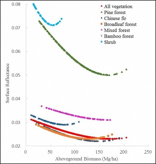
In this study, we estimated the data saturation values of Landsat 5 TM imagery for six vegetation types using a spherical model in geostatistics. We obtained and compared the values of asymptote for spherical, exponential and Gaussian models, and then derived the threshold values of the X axis, that is, saturation values of forest AGB. The idea behind these models is that as forest AGB increases, the spectral reflectance changes quickly at the beginning and then slowly and eventually becomes stable. When the spectral reflectance becomes stable, the corresponding AGB value can be regarded as the saturation value. In geostatistics, these models are used to model the spatial autocorrelation of a random variable and find the maximum distance of spatial autocorrelation. In this study, these models are considered as general models that are characterized by asymptote of the Y axis in which, by seeking the values of asymptote for the Y axis (that is, spectral reflectance of Landsat TM band 7), the range parameter values of the X axis (that is, forest AGB) are estimated. The results showed that the spherical model led to the smallest residuals and the exponential and Gaussian models resulted in much larger and unreasonable saturation values (78 Mg/ha–423 Mg/ha) than the spherical model (55 Mg/ha–159 Mg/ha). The reason is mainly because the exponential and Gaussian models theoretically have smaller change rates of the Y axis and much larger values of asymptote than the spherical model. This implies that when the spectral reflectance of Landsat band 7 becomes insensitive to the increase of forest AGB, the asymptote values of the exponential and Gaussian models are not obtained and, thus, the data saturation values are enlarged. Our results for the spherical model show that pine forests had the greatest saturation value, then mixed forests, fir, and broadleaf forests. The shrubs had the smallest saturation value. The findings are consistent with the forest status of this study area. This is a novel examination of data saturation in a subtropical region and further studies are needed in other forest ecosystems such as in tropical and temperate regions. A better understanding of the data saturation problem in different vegetation types provides a foundation to find ways to reduce saturation.
As data saturation may be caused by different factors such as remote sensing data themselves (e.g., spatial, spectral, radiometric, and temporal resolutions in optical sensor data), vegetation (e.g., species composition, stand structure, growth stages), and topography (e.g., aspects, elevation, slope), many potential solutions may be used to reduce the data saturation problem. Saturation occurs when the spectral values remain insensitive to increases in AGB beyond a certain value. An optical sensor is not able to penetrate a dense tree canopy. When all canopy gaps have been closed by leaves and branches, trees may continuously grow and their biomass continuously increases in volume without changing the spectral signature of the canopy. The AGB saturation level varies with sensor types. C-band (6 cm wavelength) synthetic aperture radar (SAR) sensors may capture canopy roughness but they are not able to penetrate beyond the top layer of leaves and thin branches. L-band (24 cm) SAR is better at penetrating the canopy, and P-band (70 cm) is even better and may capture the entire tree structure. As a rule of thumb, SAR signals may be able to penetrate structures that are narrower than the wavelength. The integration of Landsat TM and SAR data may lead to the mitigation of the data saturation problem and, thus, improve AGB estimation [21]. Further research is needed in the future to explore approaches to integrating multisensor data [67,68], especially the fusion of optical and radar or lidar data [6,21].
Lu’s study [30] has shown the importance of incorporating textures into spectral responses in improving AGB estimation performance and this research also proved the necessity of image textures. Other research using textures from the optical or SAR data provided similar conclusions [20,25,26,27,53]. The critical point is to identify specific textures for given vegetation types. This is because a good texture image for a given vegetation type depends on different factors such as spatial resolution of the remote sensing data, the complexity of forest stand structure, species composition, and the window size used for extraction of a textural image [6,30,52]. The difficulty in identifying the best textural images was encountered in this research as different textural images were used for specific vegetation types, depending on the combination of texture measures, window size, and spectral bands. Another potential approach to reducing the data saturation problem is to use different seasonal Landsat images or time series [20,34,48]. This is important because vegetation types such as pine forest, broadleaf forest, and bamboo forest have their own phenology, thus incorporation of different features inherent in vegetation phenology may be beneficial to AGB estimation.
This research indicates the important role of stratification of vegetation types and slope aspects in reducing the data saturation problem. More research is needed to identify suitable stratification approaches such as the optimal number of vegetation types and topographic factors. The key is to obtain a sufficient number of sample plots for each stratum. More strata require more sample plots, which is often a challenge because of the difficulty, time-consumption, and cost of collecting sample plots for AGB calculation. Also, a number of strata may be unnecessary, as shown in Table 10 whereby the regression models look similar for pine and fir in shady and semi-shady slopes. This raises a new question of how many strata are optimal considering the required number of sample plots for each stratum, the accuracy of AGB estimates, vegetation types, and the time and labor involved in developing AGB estimation models. To date, no studies have identified the optimal strata based on availability of sample plots, vegetation data, and ancillary data. Since vegetation types are required for stratification, accurate classification is needed, and 85% is regarded as a standard [
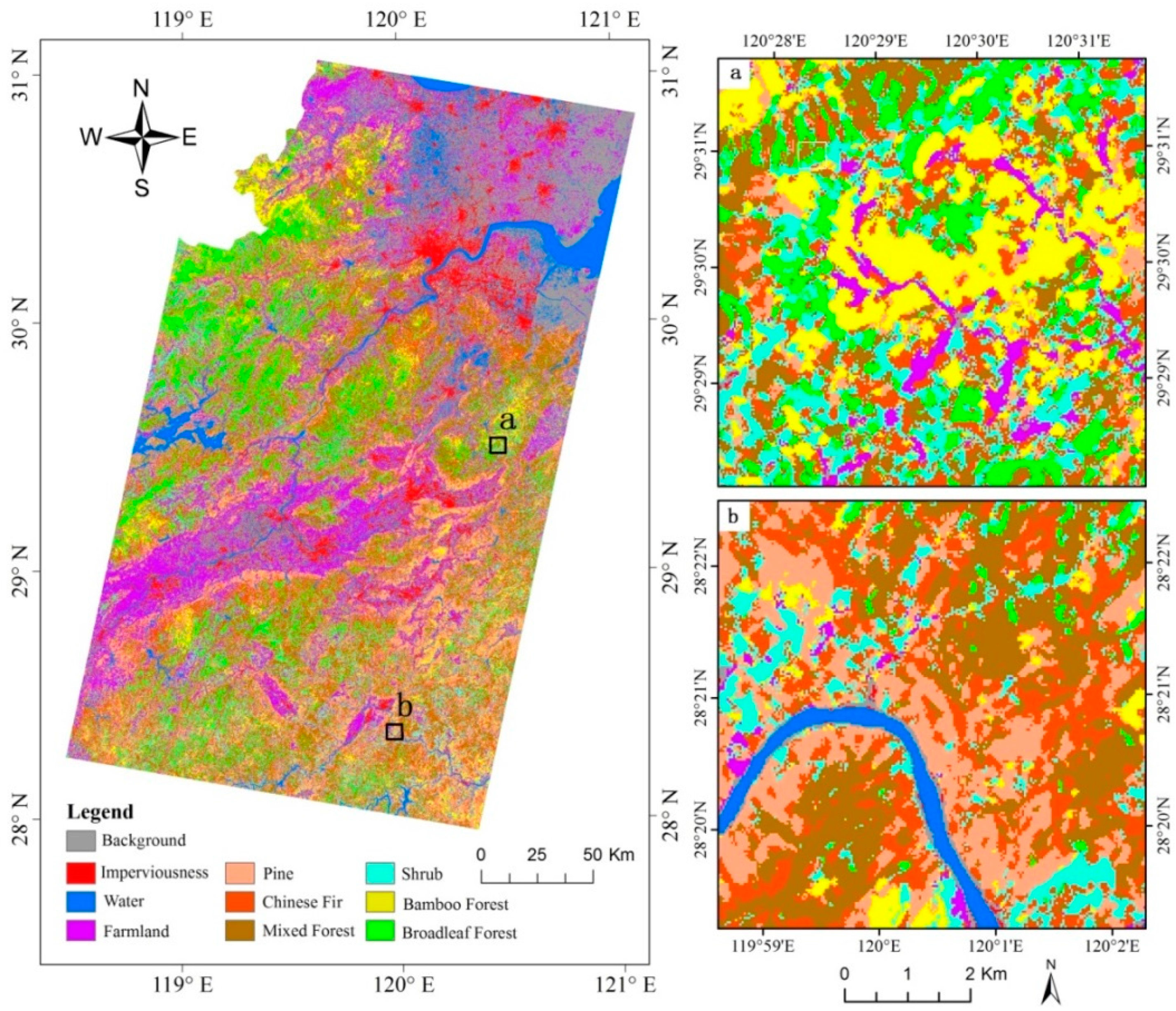
69]. In this research, six vegetation types—pine, fir, broadleaf, mixed forest, bamboo, and shrub—were classified using MLC with an overall classification accuracy of 78%. Because the vegetation types were used as stratification for developing AGB estimation models for each vegetation type, higher classification accuracy of these vegetation types is needed; but in reality, it is a challenge to produce highly accurate classification results based on Landsat TM spectral signatures due to the spectral confusion between the vegetation types and the impacts of topographic factors. In the near future, we will incorporate other data sources such as DEM, Landsat, and SAR to improve classification accuracy.
The findings about the data saturation values in different vegetation types and potential solutions to reduce the saturation problem may provide new insights into the selection of remote sensing data or design of spectral wavelengths in the future. This research indicated that shortwave infrared bands such as Landsat 5 TM bands 5 and 7 have strong relationships with AGB. More research is needed to relate this research to hyperspectral data to identify more sensitive spectral bands corresponding to different vegetation types.

5.2. Selection of Suitable Algorithms to Establish the Relationship between AGB and Remote Sensing Variables

Linear regression analysis is often used to develop AGB estimation models [4,6]. In this study, most of the determination coefficients R2 varied from 0.35 to 0.5 for all the forest AGB models and, as expected, the results are similar to those in other studies [
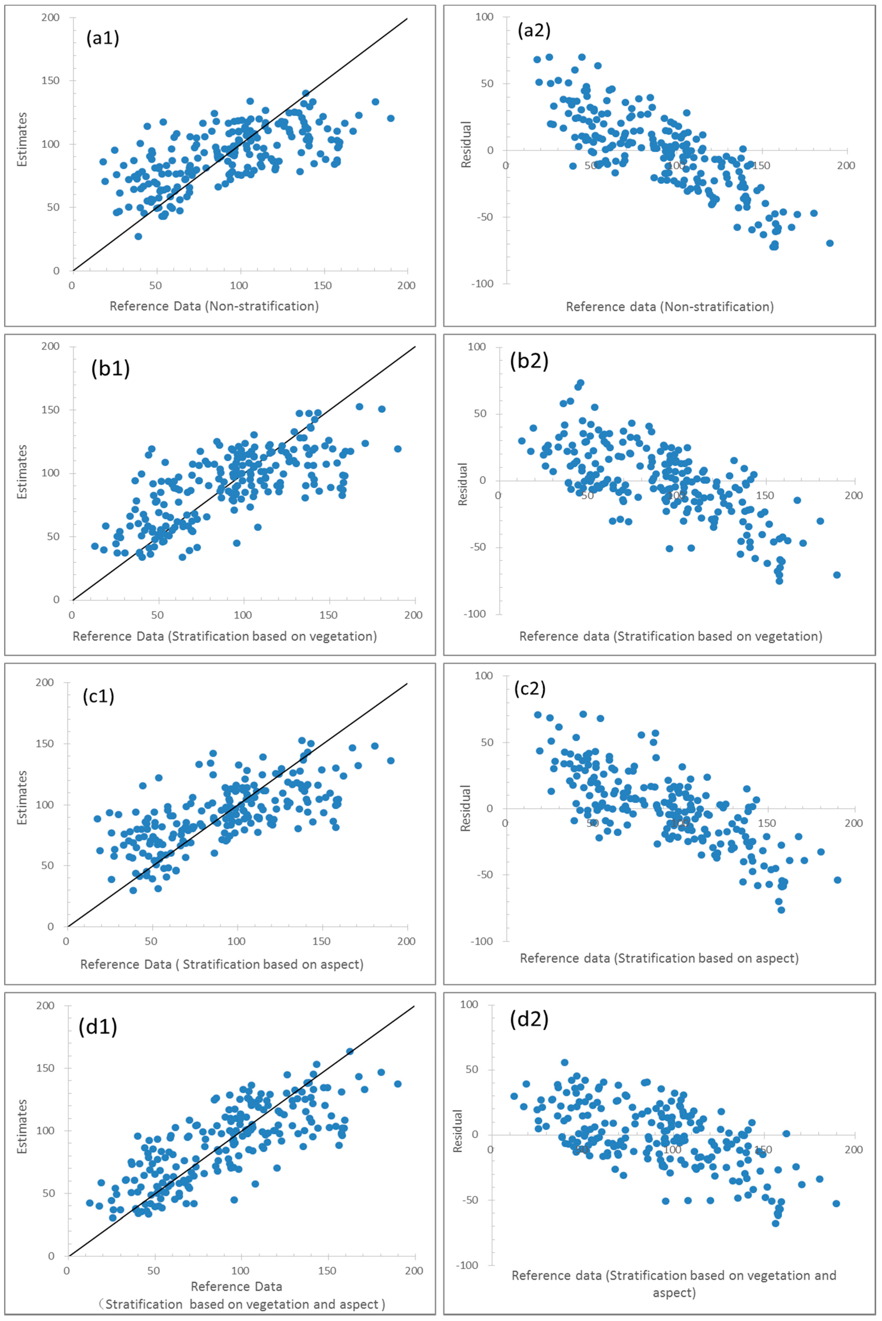
70]. However, the relationship between residuals and AGB reference data has linear features, that is, overestimations and underestimations for the smaller and larger observations, respectively (see Figure 7), pointing to the problem of using linear-based regression models. The overestimations and underestimations were mainly caused by global regression modeling. Moreover, the data saturation of Landsat spectral reflectance may have greatly contributed to the underestimations of AGB for the larger observations. Appropriate algorithms should be further studied to reduce the overestimations and underestimations. There are several potential alternatives in algorithms. First, different source data such as optical images and their textural variables, radar, lidar, topographic variables (slope and aspect) from DEM, soil properties, and vegetation types can be combined to model their relationships with AGB and improve the accuracy of predictions [6,32]. Second, the relationships between AGB and independent variables can be modeled after stratification of a study area [71].
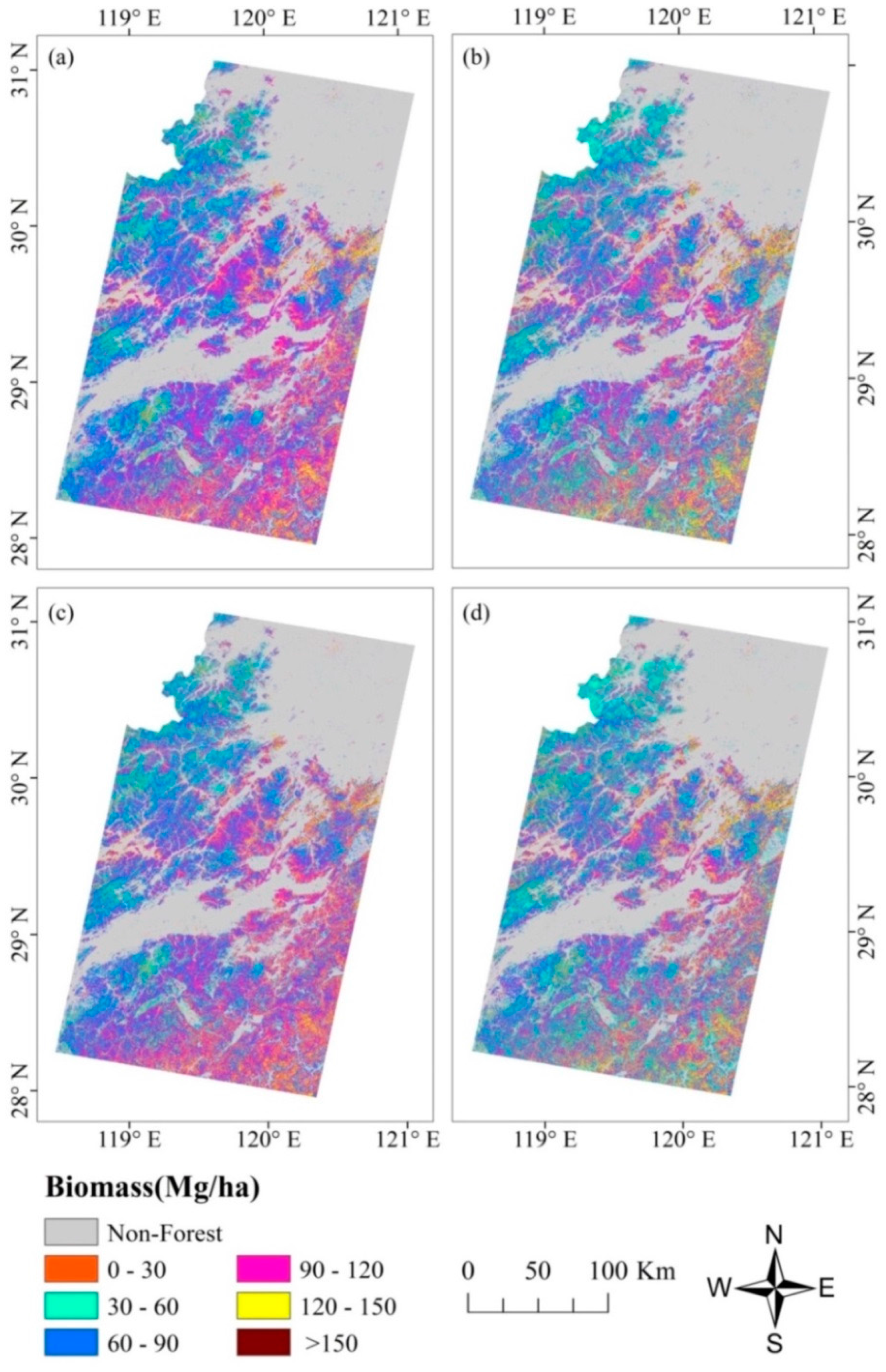
In this study, compared to non-stratification, the stratification of vegetation types and slope aspects led to the decrease of RMSEr based on the validation dataset. However, the obvious overestimations and underestimations for the smaller and larger observations, respectively, were still noticed. One purpose of stratification is to reduce the errors due to the global regression modeling by minimizing the within-strata variability and maximizing the between-strata variance [71]. In this study, the stratification of vegetation types and slope aspects did, to some extent, increase the accuracy of AGB estimates. However, because of the large area and complicated landscapes, the within-strata variability of AGB for each of the vegetation types was still large and this was especially true for the young and mature forests, resulting in high overestimations in young forests and underestimations in mature forests. Therefore, the third set of alternative algorithms may be the use of local modeling methods such as geographically weighted regression, co-kriging, and spatial co-simulation in geostatistics. In these local modeling algorithms, models are developed using the nearest sample plots within a neighborhood of a given radius. The neighborhood can be determined using the range of spatial autocorrelation. For the geographically weighted regression, the parameters of obtaining regression models will vary from place to place. Similarly, the co-kriging and spatial co-simulation will lead to variable weights of sample data. That is, the local modeling algorithms can capture the spatial variability of local areas and, thus, have great potential to reduce the overestimations and underestimations [7,71,72,73,74]. There is also a simple way to reduce the linear bias of AGB estimates in which the sample plots that are at saturation can be excluded and a simple linear regression of the data that are not saturated in Landsat imagery can be then developed for each vegetation type. With this approach, the saturated data in Landsat imagery could be flagged as saturated. This research indicated that overestimation is obvious when AGB is less than 40 Mg/ha. When AGB is small, the sites are mainly shrub, bamboo forest, new plantations, and young broadleaf forests, where vegetation canopy is not sufficiently dense, thus soil will influence surface reflectance. Previous research has indicated that a forest site can be assumed as a combination of green vegetation, shade, soil, and nonphotosynthetic vegetation (e.g., stem, braches), and these components can be decomposed using spectral mixture analysis [22,31].
Stratification led to a decrease of sample plots for each stratum, and decreasing the number of sample plots generally improves the performance of the model. Thus, the improvement of the models based on the stratifications is related to not only the relationships between forest AGB and spectral variables, but also the sample size effect. To map AGB of African forests using a sample size of 26 plots, for example, Bastin et al. [75] tested the effect of sample size on performance of the models. However, the effect of sample size may be obvious when a small sample size (such as <30 plots) is utilized. As the sample size increases, the effect of sample size should gradually disappear. In this study, 589 sample plots and 213 sample plots were respectively used for developing and validating the models (Table 3). When modeling was carried out based on stratification of vegetation types, large sample sizes were employed for all vegetation types except shrub. When modeling was conducted based on stratification of both vegetation types and slope aspects, most sample sizes were larger than 30 except bamboo and shrub relevant strata (Table 3). Thus, in this study, we discarded the development of the models based on the stratification of slope aspects for bamboo and shrub, and the effects of sample sizes on performance of the models for other strata were ignored. In this study, pixel level predictions were conducted partly because spatially explicit estimates are needed for advanced and digital forest inventory, monitoring, and management, and partly because the detailed spatial distributions of forest AGB estimates can provide the opportunity to identify the areas with smaller and larger values of biomass and corresponding uncertainties of potential overestimations and underestimation. Especially, the areas of greater estimates indicate a higher possibility of data saturation. If only the estimates of large or small areas are of interest, and not pixel level predictions, combining post-stratification and spatial modeling or other synthetic or small area estimation methods may constitute more feasible approaches. Data saturation analyses may be less important. On the other hand, the estimates obtained with the approach used in this study may be improved using some kind of calibration technique.
In addition, the stepwise regression approach used in this study tends to increase the risk of overfitting, that is, a model accounts for random error or noise instead of the underlying relationship. When too many independent variables relative to the number of used observations are involved, overfitting will very likely take place and the resulting model will perform poorly in making predictions. In this study, in the case of non-stratification, a large number of observations was used and overfitting would not have occurred. However, in the case of stratification of vegetation types and slope aspects, the number of observations for some strata such as bamboo and shrub were relatively small and the overfitting probably would have happened, which might have led to uncertainties of the estimates. Algorithms that can be used to avoid overfitting include the use of cross-validation, regularization, pruning, and model comparison. This issue should be examined in future research.

5.3. Uncertainties Due to Sample Plots

In this study, field observations of AGB were collected from 20 m × 20 m sample plots, which were smaller than the 30 m × 30 m spatial resolution of the Landsat TM images. The small plot size tends to increase the coefficient of variation of AGB, consequently leading to potential underestimations or overestimations of forest AGB at the plot level and potential non-normal distribution of AGB at the landscape level [76]. Unfortunately, the number of uncertainties due to the small plots in this study could not be quantified. However, the analysis of histograms based on plot-level observations and landscape level estimates of forest AGB showed that the distributions of AGB were close to normal. Moreover, although in this study the central coordinates of the sample plots were utilized to extract the values of image pixels, the small plot size and its inconsistency with the spatial resolution of Landsat TM images have probably induced errors in plot geolocalization and match with image pixels, and, thus, uncertainties of forest AGB estimates [77]. This could become more serious as the texture measures from the windows of 3 × 3 pixels, 5 × 5 pixels, etc., are employed. Wang and Zhang [78,79] studied the uncertainty due to error of plot geolocalization and mismatch of sample plots with image pixels and found that, as the distance of the mismatch increased, the estimation accuracy of forest AGB or carbon density obviously decreased.
In reality, the plot size of 20 m × 20 m is commonly used in forest inventory considering the work load required during fieldwork and its representativeness in a forest site. In order to reduce the errors between geolocalization of sample plots and Landsat imagery, a window size of 3 × 3 pixels was often used [6,30] to extract the remotely sensed mean values [30]. In this research, each sample plot was first examined to make sure each plot was located within the forest sites and had good representation of the surveyed forest stand. In addition to the plot size and geolocation error, another critical factor is the use of allometric models for AGB calculation for each plot based on field measurement [80]. Improper selection of the allometric models for specific tree species may produce high uncertainty of AGB calculation at the plot level, thus affecting the AGB estimation performance using the remote sensing data.

6. Conclusions

Data saturation in Landsat imagery is well recognized as a major problem resulting in poor AGB estimation, but the exact saturation value has not been fully examined mainly due to the unavailability of sufficient groundtruth data. This research examined the Landsat 5 TM data saturation problem in a subtropical region in Zhejiang province of Eastern China using sample plots for six vegetation types. Results indicate that vegetation in this study area had AGB saturation of 156 Mg/ha, pointing to the difficulty of AGB estimation using Landsat imagery when the AGB is higher than this saturation value. Meanwhile, different vegetation types have various AGB saturation values, for example, pine has the highest value of 159 Mg/ha, followed by mixed forest with an AGB saturation value of 152 Mg/ha. The bamboo forest and shrub have the lowest AGB saturation values of 75 and 55 Mg/ha, respectively. This research implies the importance of addressing the data saturation problem to improve AGB estimation when Landsat imagery is used.
Because different vegetation types have various forest stand structures and tree species compositions, they have various AGB saturation values. Meanwhile, topography produces different moisture and soil conditions, as well as solar illumination conditions, thus resulting in different growth rates and forest stand structures. This research explored the AGB estimation models using the stratification of vegetation types and slope aspects, and has shown that this kind of stratification is useful in improving AGB estimation performance. The RMSE can be reduced from 29.3 to 24.5 Mg/ha by stratification of vegetation type and slope aspect compared with the results of non-stratification. The stratification of vegetation types is especially valuable for improving AGB estimation for the forest sites with small AGB values, and the stratification of slope aspects is valuable for improving AGB estimation when AGB is greater than 160 Mg/ha, that is, when AGB reaches saturation in Landsat TM imagery. This research implies that stratification based on vegetation types and/or slope aspects can reduce the AGB saturation problem in Landsat TM imagery, thus, improving AGB estimation performance. More research is needed to address the data saturation problem by integrating multisensor/resolution remotely sensed data and ancillary data such as from DEM.

Acknowledgments

This study was financially supported by the National Natural Science Foundation of China (grant #41571411), Zhejiang Agriculture and Forestry University’s Research and Development Fund for the talent startup project (grant #2013FR052). Chuping Wu and Yujie Huang acknowledge the financial support from the Zhejiang Provincial Forestry Department (grant #2014SY01) and Shuquan Yu acknowledges the financial support from the Zhejiang Provincial Center for Forestry Ecosystem and Engineering Management for the collection of sample plots.

Author Contributions

Panpan Zhao performed the experiments and analyzed the data; Dengsheng Lu and Guangxing Wang conceived and designed the experiments, analyzed the data, and wrote the paper; Chuping Wu, Yujie Huang, and Shuquan Yu conducted sample plot collection and calculation of aboveground biomass at the plot level.

Conflicts of Interest

The authors declare no conflicts of interest. The funding sponsors had no role in the design of the study; the collection, analyses, or interpretation of data; the writing of the manuscript; or the decision to publish the results.

References

  1. IPCC (Intergovernmental Panel on Climate Change). Land Use, Land-Use Change and Forestry; Cambridge Univ. Press: Cambridge, UK, 2000. [Google Scholar]
  2. Smith, J.E.; Heath, L.S. Carbon Stocks and Stock Changes in U.S. Forests and appendix C. In U.S. Agriculture and Forestry Greenhouse Gas Inventory: 1990–2005; Global Change Program Office, Office of the Chief Economist: Washington, DC, USA; Technical Bulletin No. 1921; 2008. Available online: http://www.usda.gov/oce/global_change/ AFGGInventory1990_2005.htm (accessed on 28 August 2015). [Google Scholar]
  3. US Climate Change Science Program. The North American Carbon Budget and Implications for the Global Carbon Cycle. 2007. Available online: http://www.cfr.org/climate-change/north-american-carbon-budget-implications-global-carbon-cycle/p14868 (accessed on 28 August 2015).
  4. Lu, D. The potential and challenge of remote sensing-based biomass estimation. Int. J. Remote Sens. 2006, 27, 1297–1328. [Google Scholar] [CrossRef]
  5. Lu, D.; Chen, Q.; Wang, G.; Moran, E.; Batistella, M.; Zhang, M.; Laurin, G.V.; Saah, D. Aboveground forest biomass estimation with Landsat and LiDAR data and uncertainty analysis of the estimates. Int. J. For. Res. 2012, 1–16. [Google Scholar] [CrossRef]
  6. Lu, D.; Chen, Q.; Wang, G.; Liu, L.; Moran, E. A survey of remote sensing-based aboveground biomass estimation methods. Int. J. Digit. Earth 2016, 9, 63–105. [Google Scholar] [CrossRef]
  7. Wang, G.; Oyana, T.; Zhang, M.; Adu-Prah, S.; Zeng, S.; Lin, H.; Se, J. Mapping and spatial uncertainty analysis of forest vegetation carbon by combining national forest inventory data and satellite images. For. Ecol. Manag. 2009, 258, 1275–1283. [Google Scholar] [CrossRef]
  8. Landsberg, J.J.; Waring, R.H. A generalized model of forest productivity using simplified concepts of radiation-use efficiency, carbon balance, and partitioning. For. Ecol. Manag. 1997, 95, 209–228. [Google Scholar] [CrossRef]
  9. Running, S.W.; Coughlan, J.C. A general model of forest ecosystem processes for regional applications I. hydrologic balance, canopy gas exchange and primary production processes. Ecol. Model. 1988, 42, 125–154. [Google Scholar] [CrossRef]
  10. Kimball, J.S.; Keyser, A.R.; Running, S.W.; Saatch, S.S. Regional assessment of boreal forest productivity using an ecological process model and remote sensing parameter maps. Tree Physiol. 2000, 20, 761–775. [Google Scholar] [CrossRef] [PubMed]
  11. Kumar, L.; Sinha, P.; Taylor, S.; Alqurashi, A.F. Review of the use of remote sensing for biomass estimation to support renewable energy generation. J. Appl. Remote Sens. 2015, 9, 29. [Google Scholar] [CrossRef]
  12. Barbosa, J.M.; Broadbent, E.N.; Bitencourt, M.D. Remote sensing of aboveground biomass in tropical secondary forests: A review. Int. J. For. Res. 2014, 14. [Google Scholar] [CrossRef]
  13. Timothy, D.; Onisimo, M.; Cletah, S.; Adelabu, S.; Tsitsi, B. Remote sensing of aboveground forest biomass: A review. Trop. Ecol. 2016, 57, 125–132. [Google Scholar]
  14. Timothy, D.; Onisimo, M.; Riyad, I. Quantifying aboveground biomass in African environments: A review of the trade-offs between sensor estimation accuracy and costs. Trop. Ecol. 2016, 57, 393–405. [Google Scholar]
  15. Vashum, K.T.; Jayakumar, S. Methods to estimate aboveground biomass and carbon stock in natural forests—A review. J. Ecosyst. Ecogr. 2012, 2, 116. [Google Scholar] [CrossRef]
  16. Goetz, S.J.; Baccini, A.; Laporte, N.T.; Johns, T.; Walker, W.; Kellndorfer, J.; Houghton, R.A.; Sun, M. Mapping and monitoring carbon stocks with satellite observations: A comparison of methods. Carbon Balance Manag. 2009, 4, 2. [Google Scholar] [CrossRef] [PubMed]
  17. Song, C. Optical remote sensing of forest leaf area index and biomass. Prog. Phys. Geogr. 2012, 37, 98–113. [Google Scholar] [CrossRef]
  18. Muukkonen, P.; Heiskanen, J. Estimating biomass for boreal forests using ASTER satellite data combined with standwise forest inventory data. Remote Sens. Environ. 2005, 99, 434–447. [Google Scholar] [CrossRef]
  19. Muukkonen, P.; Heiskanen, J. Biomass estimation over a large area based on standwise forest inventory data and ASTER and MODIS satellite data: A possibility to verify carbon inventories. Remote Sens. Environ. 2007, 107, 617–624. [Google Scholar] [CrossRef]
  20. Gasparri, N.I.; Parmuchi, M.G.; Bono, J.; Karszenbaum, H.; Montenegro, C.L. Assessing multitemporal Landsat 7 ETM+ images for estimating aboveground biomass in subtropical dry forests of Argentina. J. Arid Environ. 2010, 74, 1262–1270. [Google Scholar] [CrossRef]
  21. Cutler, M.E.J.; Boyd, D.S.; Foody, G.M.; Vetrivel, A. Estimating tropical forest biomass with a combination of SAR image texture and Landsat TM data: An assessment of predictions between regions. ISPRS J. Photogramm. Remote Sens. 2012, 70, 66–77. [Google Scholar] [CrossRef] [Green Version]
  22. Fernández-Manso, O.; Fernández-Manso, A.; Quintano, C. Estimation of aboveground biomass in Mediterranean forests by statistical modelling of ASTER fraction images. Int. J. Appl. Earth Observ. Geoinf. 2014, 31, 45–56. [Google Scholar] [CrossRef]
  23. Güneralp, I.; Filippi, A.M.; Randall, J. Estimation of floodplain aboveground biomass using multispectral remote sensing and nonparametric modeling. Int. J. Appl. Earth Observ. Geoinf. 2014, 33, 119–126. [Google Scholar] [CrossRef]
  24. Gömez, C.; White, J.C.; Wulder, M.A.; Alejandro, P. Historical forest biomass dynamics modelled with Landsat spectral trajectories. ISPRS J. Photogramm. Remote Sens. 2014, 93, 14–28. [Google Scholar] [CrossRef] [Green Version]
  25. Sarker, L.R.; Nichol, J.E. Improved forest biomass using ALOS AVNIR-2 texture indices. Remote Sens. Environ. 2011, 115, 968–977. [Google Scholar] [CrossRef]
  26. Dube, T.; Mutanga, O. Investigating the robustness of the new Landsat-8 Operational Land Imager derived texture metrics in estimating plantation forest aboveground biomass in resource constrained areas. ISPRS J. Photogramm. Remote Sens. 2015, 108, 12–32. [Google Scholar] [CrossRef]
  27. Kelsey, K.C.; Neff, J.C. Estimates of aboveground biomass from texture analysis of Landsat imagery. Remote Sens. 2014, 6, 6407–6422. [Google Scholar] [CrossRef]
  28. Dube, T.; Mutanga, O. Evaluating the utility of the medium-spatial resolution Landsat 8 multispectral sensor in quantifying aboveground biomass in uMgeni catchment, South Africa. ISPRS J. Photogramm. Remote Sens. 2015, 101, 36–46. [Google Scholar] [CrossRef]
  29. Foody, G.M.; Boyd, D.S.; Cutler, M.E. Predictive relations of tropical forest biomass from Landsat TM data and their transferability between regions. Remote Sens. Environ. 2003, 85, 463–474. [Google Scholar] [CrossRef]
  30. Lu, D. Aboveground biomass estimation using Landsat TM data in the Brazilian Amazon. Int. J. Remote Sens. 2005, 26, 2509–2525. [Google Scholar] [CrossRef]
  31. Lu, D.; Batistella, M.; Moran, E. Satellite estimation of aboveground biomass and impacts of forest stand structure. Photogramm. Eng. Remote Sens. 2005, 71, 967–974. [Google Scholar] [CrossRef]
  32. Avitabile, V.; Baccini, A.; Friedl, M.A.; Schmullius, C. Capabilities and limitations of Landsat and land cover data for aboveground woody biomass estimation of Uganda. Remote Sens. Environ. 2012, 117, 366–380. [Google Scholar] [CrossRef]
  33. Ji, L.; Wylie, B.K.; Nossov, D.R.; Peterson, B.; Waldrop, M.P.; McFarland, J.W.; Rover, J.; Hollingsworth, T.N. Estimating aboveground biomass in interior Alaska with Landsat data and field measurements. Int. J. Appl. Earth Observ. Geoinf. 2012, 18, 451–461. [Google Scholar] [CrossRef]
  34. Powell, S.L.; Cohen, W.B.; Healey, S.P.; Kennedy, R.E.; Moisen, G.G.; Pierce, K.B.; Ohmann, J.L. Quantification of live aboveground forest biomass dynamics with Landsat time-series and field inventory data: A comparison of empirical modeling approaches. Remote Sens. Environ. 2010, 114, 1053–1068. [Google Scholar] [CrossRef]
  35. Hall, R.J.; Skakun, R.S.; Arsenault, E.J.; Case, B.S. Modeling forest stand structure attributes using Landsat ETM+ data: Application to mapping of aboveground biomass and stand volume. For. Ecol. Manag. 2006, 225, 378–390. [Google Scholar] [CrossRef]
  36. Labrecque, S.; Fournier, R.A.; Luther, J.E.; Piercey, D. A comparison of four methods to map biomass from Landsat-TM and inventory data in western Newfoundland. For. Ecol. Manag. 2006, 226, 129–144. [Google Scholar] [CrossRef]
  37. Duncanson, L.I.; Niemann, K.O.; Wulder, M.A. Integration of GLAS and Landsat TM data for aboveground biomass estimation. Can. J. Remote Sens. 2010, 36, 129–141. [Google Scholar] [CrossRef]
  38. Baccini, A.; Laporte, N.; Goetz, S.J.; Sun, M.; Dong, H. A first map of tropical Africa’s above-ground biomass derived from satellite imagery. Environ. Res. Lett. 2008, 3, 045011. [Google Scholar] [CrossRef]
  39. Blackard, J.A.; Finco, M.V.; Helmer, E.H.; Holden, G.R.; Hoppus, M.L.; Jacobs, D.M.; Lister, A.J.; Moisen, G.G.; Nelson, M.D.; Riemann, R.; et al. Mapping U.S. forest biomass using nationwide forest inventory data and moderate resolution information. Remote Sens. Environ. 2008, 112, 1658–1677. [Google Scholar] [CrossRef]
  40. Boyd, D.S.; Foody, G.M.; Curran, P.J. The relationship between the biomass of Cameroonian tropical forests and radiation reflected in middle infrared wavelengths (3.0-5.0 mu m). Int. J. Remote Sens. 1999, 20, 1017–1023. [Google Scholar] [CrossRef]
  41. Tian, X.; Su, Z.; Chen, E.; Li, Z.; van der Tol, C.; Guo, J.; He, Q. Estimation of forest aboveground biomass using multi-parameter remote sensing data over a cold and arid area. Int. J. Appl. Earth Observ. Geoinf. 2012, 14, 160–168. [Google Scholar] [CrossRef]
  42. Zheng, D.; Rademacher, J.; Chen, J.; Crow, T.; Bresee, M.; le Moine, J.; Ryu, S. Estimating aboveground biomass using Landsat 7 ETM+ data across a managed landscape in northern Wisconsin, USA. Remote Sens. Environ. 2004, 93, 402–411. [Google Scholar] [CrossRef]
  43. Xie, Y.; Sha, Z.; Yu, M.; Bai, Y.; Zhang, L. A comparison of two models with Landsat data for estimating above ground grassland biomass in Inner Mongolia, China. Ecol. Model. 2009, 220, 1810–1818. [Google Scholar] [CrossRef]
  44. Foody, G.M.; Cutler, M.E.; McMorrow, J.; Pelz, D.; Tangki, H.; Boyd, D.S.; Douglas, I. Mapping the biomass of Bornean tropical rain forest from remotely sensed data. Glob. Ecol. Biogeogr. 2001, 10, 379–387. [Google Scholar] [CrossRef]
  45. Chander, G.; Markham, B.L.; Helder, D.L. Summary of current radiometric calibration coefficients for Landsat MSS, TM, ETM+, and EO-1 ALI sensors. Remote Sens. Environ. 2009, 113, 893–903. [Google Scholar] [CrossRef]
  46. Reese, H.; Olsson, H. C-correction of optical satellite data over alpine vegetation areas: A comparison of sampling strategies for determining the empirical c-parameter. Remote Sens. Environ. 2011, 115, 1387–1400. [Google Scholar] [CrossRef]
  47. Lu, D.; Weng, Q. A survey of image classification methods and techniques for improving classification performance. Int. J. Remote Sens. 2007, 28, 823–870. [Google Scholar] [CrossRef]
  48. Zhu, X.; Liu, D. Improving forest aboveground biomass estimation using seasonal Landsat NDVI time-series. ISPRS J. Photogramm. Remote Sens. 2015, 102, 222–231. [Google Scholar] [CrossRef]
  49. Nichol, J.E.; Sarker, M.L.R. Improved biomass estimation using the texture parameters of two high-resolution optical sensors. IEEE Trans. Geosci. Remote Sens. 2011, 49, 930–948. [Google Scholar] [CrossRef]
  50. Sarker, M.L.R.; Nichol, J.; Ahmad, B.; Busu, I.; Rahman, A.A. Potential of texture measurements of two-date dual polarization PALSAR data for the improvement of forest biomass estimation. ISPRS J. Photogram. Remote Sens. 2012, 69, 146–166. [Google Scholar] [CrossRef]
  51. Lu, D.; Mausel, P.; Brondízio, E.; Moran, E. Relationships between forest stand parameters and Landsat Thematic Mapper spectral responses in the Brazilian Amazon basin. For. Ecol. Manag. 2004, 198, 149–167. [Google Scholar] [CrossRef]
  52. Lu, D.; Batistella, M. Exploring TM image texture and its relationships with biomass estimation in Rondônia, Brazilian Amazon. Acta Amazôn. 2005, 35, 249–257. [Google Scholar] [CrossRef]
  53. Kuplich, T.M.; Curran, P.J.; Atkinson, P.M. Relating SAR image texture to the biomass of regenerating tropical forests. Int. J. Remote Sens. 2005, 26, 4829–4854. [Google Scholar] [CrossRef]
  54. Sanga-Ngoie, K.; Iizuka, K.; Kobayashi, S. Estimating CO2 sequestration by forests in Oita prefecture, Japan, by combining Landsat ETM plus and ALOS Satellite remote sensing data. Remote Sens. 2012, 4, 3544–3570. [Google Scholar] [CrossRef]
  55. Zhejiang. Available online: https://en.wikipedia.org/wiki/Zhejiang/ (accessed on 26 February 2016).
  56. Zhu, T.; Shen, C.; Ji, B.; Lin, Y.; Wang, X.; Zhang, G.; Yuan, W. Biomass conversion coefficients of Chinese fir forests of Zhejiang Province based on LULUCF greenhouse gas emission. Acta Ecol. Sin. 2013, 33, 3925–3932. (In Chinese) [Google Scholar]
  57. Forestry Department of Zhejiang Province: Introduction of Forestry. Available online: http://baike.baidu.com/view/4532835.htm#5 (accessed on 26 February 2016).
  58. Qia, Y.; Yi, L.; Zhang, C.; Yu, S.; Shen, L.; Pan, D.; Deng, C. Bioass and carbon stocks of commonwealth forests for Central Zhejiang. For. Sci. 2013, 49, 17–23. (In Chinese) [Google Scholar]
  59. Yuan, W.; Jiang, B.; Ge, Y.; Zhu, J.; Shen, A. Study on biomass models of important commonwealth forests for Zhejiang Province. J. Zhejiang For. Technol. 2009, 29, 1–5. (In Chinese) [Google Scholar]
  60. Li, C.; Fan, J.; Fu, X.; Fan, H. Analysis and comparison test on C-correction strategies and their scale effects with TM images in rugged mountainous terrain. J. Geo-Inf. Sci. 2014, 16, 134–141. [Google Scholar]
  61. Li, G.; Lu, D.; Moran, E.; Sant’Anna, S.J.S. A comparative analysis of classification algorithms and multiple sensor data for land use/land cover classification in the Brazilian Amazon. J. Appl. Remote Sens. 2012, 6, 061706. [Google Scholar] [CrossRef]
  62. Lu, D.; Li, G.; Kuang, W.; Moran, E. Methods to extract impervious surface areas from satellite images. Int. J. Digit. Earth 2014, 7, 93–112. [Google Scholar] [CrossRef]
  63. Li, L.; Lu, D.; Kuang, W. Examining urban impervious surface distribution and its dynamic change in Hangzhou metropolis. Remote Sens. 2016, 8, 265. [Google Scholar] [CrossRef]
  64. Xu, H. A study on information extraction of water body with the modified normalized difference water index (MNDWI). J. Remote Sens. 2005, 5, 589–595. [Google Scholar]
  65. Congalton, R.G.; Green, K. Assessing the Accuracy of Remotely Sensed Data: Principles and Practices, 2nd ed.; CRC Press: Boca Raton, FL, USA, 2008. [Google Scholar]
  66. McRoberts, R.E.; Næsset, E.; Gobakken, T. Inference for lidar-assisted estimation of forest growing stock volume. Remote Sens. Environ. 2013, 128, 268–275. [Google Scholar] [CrossRef]
  67. Zhang, J. Multi-source remote sensing data fusion: Status and trends. Int. J. Image Data Fusion 2010, 1, 5–24. [Google Scholar] [CrossRef]
  68. Khaleghi, B.; Khamis, A.; Karray, F.O.; Razavi, S.N. Multisensor data fusion: A review of the state-of-the-art. Inf. Fusion 2013, 14, 28–44. [Google Scholar] [CrossRef]
  69. Andersen, J.R.; Hardy, E.E.; Roach, J.T.; Witmer, R.E. A Land Use and Land Cover Classification System for Use with Remote Sensor Data; U.S. Geological Survey Professional Paper 964; United States Government Printing Office: Washington, DC, USA, 1976. Available online: http://www.pbcgis.com/data_basics/anderson.pdf (accessed on 7 April 2016).
  70. Fleming, A.; Wang, G.; McRoberts, R. Comparison of methods toward multi-scale forest carbon mapping and spatial uncertainty analysis: Combining national forest inventory plot data and Landsat TM images. Eur. J. For. Res. 2015, 134, 125–137. [Google Scholar] [CrossRef]
  71. Wang, G.; Wente, S.; Gertner, G.; Anderson, A.B. Improvement in mapping vegetation cover factor for universal soil loss equation by geo-statistical methods with Landsat TM images. Int. J. Remote Sens. 2002, 23, 3649–3667. [Google Scholar] [CrossRef]
  72. Fotheringham, A.S.; Brunsdon, C.; Charlton, M. Geographically Weighted Regression: The Analysis of Spatially Varying Relationships; John Wiley & Sons Ltd.: West Sussex, UK, 2002. [Google Scholar]
  73. Gao, X.; Asami, Y.; Chung, C.F. An empirical evaluation of spatial regression models. Comput. Geosci. 2006, 32, 1040–1051. [Google Scholar] [CrossRef]
  74. Zhang, L.; Gove, J.H.; Health, L.S. Spatial residual analysis of six modeling techniques. Ecol. Model. 2005, 186, 154–177. [Google Scholar] [CrossRef]
  75. Bastin, J.F.; Barbier, N.; Couteron, P.; Adams, B.; Shapiro, A.; Bogaert, J.; de Canniere, C. Aboveground biomass mapping of African forest mosaics using canopy texture analysis: Toward a regional approach. Ecol. Appl. 2014, 24, 1984–2001. [Google Scholar] [CrossRef]
  76. Clark, D.B.; Clark, D.A. Landscape-scale variation in forest structure and biomass in a tropical rain forest. For. Ecol. Manag. 2000, 137, 185–198. [Google Scholar] [CrossRef]
  77. Réjou-Méchain, M.; Muller-Landau, H.C.; Detto, M.; Thomas, S.C.; le Toan, T.; Saatchi, S.S.; Barreto-Silva, J.S.; Bourg, N.A.; Bunyavejchewin, S.; Butt, N.; et al. Local spatial structure of forest biomass and its consequences for remote sensing of carbon stocks. Biogeosciences 2014, 11, 6827–6840. [Google Scholar] [CrossRef] [Green Version]
  78. Wang, G.; Zhang, M.; Gertner, G.Z.; Oyana, T.; McRoberts, R.E.; Ge, H. Uncertainties of mapping forest carbon due to plot locations using national forest inventory plot and remotely sensed data. Scand. J. For. Res. 2011, 26, 360–373. [Google Scholar] [CrossRef]
  79. Zhang, M.; Lin, H.; Zeng, S.; Li, J.; She, J.; Wang, G. Impacts of plot location errors on accuracy of mapping and up-scaling aboveground forest carbon using sample plot and Landsat TM data. IEEE Geosci. Remote Sens. Lett. 2013, 10, 1483–1487. [Google Scholar] [CrossRef]
  80. Chen, Q.; Vaglio Laurin, G.; Valentini, R. Uncertainty of remotely sensed aboveground biomass over an African tropical forest: Propagating errors from trees to plots to pixels. Remote Sens. Environ. 2015, 160, 134–143. [Google Scholar] [CrossRef]
Figure 1. Location of study area—partial Zhejiang Province, eastern China (Note: (a) the study area is located in Eastern China; (b) the study area occupies most part of Zhejiang province; and (c) a false color composite of Landsat Thematic Mapper (TM) band 4 in red, band 3 in green, and band 2 in blue, highlighting vegetated areas in red color).
Remotesensing 08 00469 g001
Figure 2. Strategy of vegetation classification from Landsat 5 Thematic Mapper (TM) image (Note: LSMA, linear spectral mixture analysis).
Remotesensing 08 00469 g002
Figure 3. Classified map (left) of land use and land cover types for the whole study area using Landsat 5 Thematic Mapper imagery, and the selected portions (a) and (b) at a large scale to highlight the complexity and spatial distribution of vegetation types.
Remotesensing 08 00469 g003
Figure 4. The relationships between aboveground biomass (AGB) and Landsat 5 Thematic Mapper (TM) spectral band 7 surface reflectance for different vegetation types: (a) pine forest; (b) Chinese fir; (c) broadleaf forest; (d) mixed forest; (e) bamboo forest; and (f) shrub.
Remotesensing 08 00469 g004
Figure 5. The modeled relationships of Landsat 5 Thematic Mapper (TM) spectral band 7 surface reflectance against forest aboveground biomass using spherical model for estimation of the data saturation value for each vegetation type (indicated using different symbols).
Remotesensing 08 00469 g005
Figure 6. A comparison of spatial distributions of forest aboveground biomass estimates among the models using four stratification scenarios: (a) non-stratification; (b) stratification based on vegetation types; (c) stratification based on slope aspects; and (d) stratification based on the combination of vegetation types and slope aspects.
Remotesensing 08 00469 g006
Figure 7. The relationships between forest aboveground biomass (AGB) estimates and reference data (a1d1); and residuals of AGB estimates against reference data (a2d2) using four stratification scenarios: (a1,a2) non-stratification; (b1,b2) stratification based on vegetation types; (c1,c2) stratification based on slope aspects; and (d1,d2) stratification based on the combination of vegetation types and slope aspects.
Remotesensing 08 00469 g007
Table 1. A statistical summary of aboveground biomass for the sample plots.
Vegetation TypesNo. of Sample PlotsMean (Mg/ha)Standard DeviationMinimum (Mg/ha)Maximum (Mg/ha)Coef. of Variation
Pine246100.05 36.71 27.00 204.83 36.69
Fir12395.79 37.73 22.15 190.76 39.39
BLF19286.98 35.05 20.51 175.71 40.29
MDF124104.58 34.30 31.92 180.70 32.80
Bamboo8754.08 20.06 10.47 108.04 37.08
Shrub3036.68 16.71 15.12 72.60 45.55
All samples80289.61 38.39 10.47 204.83 42.84
Note: BLF, broadleaf forest; MDF, mixed forest.
Table 2. A summary of sample plots for different aboveground biomass groups.
Number of Sample PlotsNumber of Sample Plots for Each AGB Group (Mg/ha)
<4040–8080–120120–160>160
Number of sample plots8027628025516526
Sample plots for modeling5895921018111821
Sample plots for evaluation213177074475
Table 3. A summary of sample plots at different vegetation types and slope aspects for development and evaluation of aboveground biomass models.
Vegetation TypesSample Plots for Modeling Sample Plots for Modeling at Different AspectsSample Plots for Evaluation
ShadySemi-ShadySunnySemi-Sunny
Pine1854454404761
Fir912028321132
BLF1383640303254
MDF922026301632
Bamboo62221861625
Shrub2145939
All sample plots589146171147125213
Note: BLF, broadleaf forest; MDF, mixed forest.
Table 4. Descriptions of vegetation types and their forest parameters.
Vegetation TypeDescriptionAverage DBH (cm)Average Height (m)Average Age (Year)
Pine Pure or Pinus Massoniana dominant forests with a small mixture of broadleaf trees and shrubs10.67.524
Fir Pure or Cunnigjamia lanceolate (Lamb.) Hook dominant forests with very small mixture of Pinus Massoniana and shrubs 11.27.523
Mixed forestsDominant species including Schima superba Gardn. et Cham, Pinus Massoniana, Cunnigjamia lanceolate (Lamb.) Hook, Cyclobalanopsis glauca and shrubs10.27.126
Broadleaf forests Tree species including Schima superba Gardn. et Cham, Castanopsis sclerophylla (Lindl.) Schott, Cyclobalanopsis glauca, Acer, Cinnamomum camphora9.06.426
Bamboo Dominant Phyllostachys heterocycla (Carr.) Mitford cv. Pubescens forests9.310.64
Shrubshrubs8.94.312
Note: DBH, diameter at breast height.
Table 5. Accuracy assessment results of a vegetation classification.
Vegetation TypesClassification DataTotalUA%
PineFirBLFMDF Bamboo ShrubFarmland
Reference dataPine172731445721281.13
Fir14771935010970.64
BLF 3515025012019576.92
MDF 137715807019282.29
Bamboo 600385319886.73
Shrub3410636319070.00
Farmland511333476374.60
Total216101172218989856
PA%79.6376.2487.2172.4886.7364.2983.93
Note: overall classification accuracy = 78.42%; kappa coefficient = 0.74. PA, Producer’s accuracy; UA, user’s accuracy; BLF, broadleaf forest; MDF, mixed forest.
Table 6. Correlation coefficients between aboveground biomass and spectral bands.
Landsat TM Spectral BandsAll-VegetationSpecific Vegetation Types
PineFirBLFMDFBambooShrub
Green (b2)−0.43 **−0.39 **−0.38 **−0.33 **−0.27*−0.03−0.32
Red (b3)−0.35 **−0.33 **−0.34 **−0.27 **−0.07−0.16−0.19
Near infrared (NIR) (b4)−0.35 **−0.27 **−0.46 **−0.37 **−0.41 **0.09−0.07
Shortwave infrared (SWIR1) (b5)−0.54 **−0.47 **−0.59 **−0.61 **−0.50 **−0.02−0.24
Shortwave infrared (SWIR2) (b7)−0.62 **−0.51 **−0.63 **−0.65 **−0.48 **−0.18−0.40*
Note: TM, Thematic Mapper; BLF, broadleaf forest; MDF, mixed forest. ** indicates significant at 0.01 and * indicates significant at 0.05.
Table 7. A summary of aboveground biomass saturation values for different vegetation types.
All vegetationDifferent Vegetation Types
PineFirBLFMDFBambooShrub
Saturation value (Mg/ha)1561591431231527555
Note: BLF, broadleaf forest; MDF, mixed forest.
Table 8. Comparison of the adjusted coefficient of determination (Radj2) among the aboveground biomass regression models based on different scenarios.
No stratification Based on AspectsStratification Based on Slope Aspects
Shady Semi-ShadySunny Semi-Sunny
No stratification based on vegetation types0.390.450.340.390.53
Stratification based on vegetation typesPine0.340.260.340.490.36
Fir0.390.490.350.320.69
MDF0.340.550.560.170.45
BLF 0.430.510.350.460.61
Bamboo *0.06
Shrub * 0.17
Note: The * behind Bamboo and Shrub indicate that the Radj2 values based on stratification of slope aspects for bamboo forest and shrub are not listed in this table because no variables can be used in the regression models for bamboo forest and not enough sample plots were available for shrub. BLF, broadleaf forest; MDF, mixed forest.
Table 9. Summary of aboveground biomass estimation models with stratification of vegetation types.
Regression ModelRadj2Standard Coefficient
Non-stratification y = 200.657 − 1107.3Sb7 − 13.195Tb7w5ME + 19.801Tb7w9CC + ε0.39−0.398; −0.248; 0.105
Stratification based on vegetation typesPiney = 213.120 − 1465.878Sb7 − 172.253Tb5w9SM − 18.857Tb3w9ME + 27.674Tb7w9CC + ε0.34 −0.457; −0.197; −0.226; 0.152
Firy = 214.532 − 1771.135Sb7 − 16.290Tb3w5CC + ε0.39 −0.668; −0.217
MDFy = 246.916 − 376.179Sb5 − 10.721Tb5w9ME + ε0.34 −0.242; −0.403
BLF y = 195.727 − 2320.487Sb7 + 1798.578Sb3 + ε0.43 −0.788; 0.241
Bamboo y = 115.334 − 6.289Tb5w9ME + ε0.06 −0.276
Shrub y = 75.827 − 542.561Sb7 + ε0.17 −0.465
Note: Sbi, spectral band i of Landsat 5 TM imagery; Tbiwjxx, textural image developed from spectral band i with a window size of jxj pixels using texture measures mean (ME), correlation (CC), or second moment (SM); ε, the residual. BLF, broadleaf forest; MDF, mixed forest.
Table 10. Summary of aboveground biomass estimation models with stratification of the combined vegetation types and slope aspects.
Shady SlopeSemi-Shady Slope
Regression ModelRadj2Std. coef.Regression ModelRadj2Std. coef.
Non-stratificationy = 232.486 − 2161.441Sb7 + ε0.45−0.673y = 205.790 − 1222.626Sb7 − 12.269Tb7w9ME + ε0.34−0.410; −0.240
Stratification based on vegetation typePiney = 229.333 − 2121.672Sb7 + ε0.26 −0.523y = 185.550 − 1733.399Sb7 + ε0.34 −0.594
Firy = 243.811 − 2380.771Sb7 + ε0.49 −0.716y = 208.571 − 1766.397Sb7 + ε0.35 −0.612
MDFy = 250.259 − 826.914Sb5 − 55.726Tb2w9SM + ε0.55 −0.604; −0.411y = 235.731 − 42.403Tb7w9ME + ε0.56 −0.763
BLFy = 349.489-927.201Sb5 − 30.386Tb7w5ME + ε0.51 −0.420; −0.401y = 236.037 − 2305.834Sb7 + ε0.35 −0.601
Sunny slopeSemi−sunny slope
Non- stratificationy = 209.005-428.519Sb5 − 17.648Tb7w5ME + 24.818Tb7w9CC + ε0.39−0.319; −0.334; 0.143y = 217.710 − 1660.365Sb7 + 1539.191Sb3 − 32.588Tb4w5CC − 26.282Tb3w9ME − 27.517Tb2w5SM + ε0.53−0.717; 0.263; −0.212; −0.306; −0.183;
Stratification based on vegetation typePiney = 189.670 − 1355.797Sb7 + ε0.49 −0.708y = 207.651 − 1016.638Sb5 + 41.957Tb7w9CC + ε0.36 −0.571; 0.241
Firy = 206.696 − 712.373Sb5 − 35.088Tb2w5CC + ε0.32 −0.500; −0.319y = 177.688 − 1482.658Sb7 + ε0.69 −0.846
MDFy = 195.701 − 26.585Tb7w5ME + ε0.17 −0.445y=226.899 − 14.984Tb5w5ME + ε0.45 −0.699
BLFy = 203.738 − 1845.973Sb7 + ε0.46 −0.693y = 188.577 − 1294.233Sb7 − 37.938Tb4w5CC + ε0.61 −0.681; −0.281
Note: Sbi, ith band of Landsat 5 TM image; Tbiwjxx, textural image from the ith band with a window size of j by j pixels using texture measures mean (ME), correlation (CC), or second moment (SM); ε, the residual. BLF, broadleaf forest; MDF, mixed forest.
Table 11. Summary of accuracy assessment results based on different stratification scenarios.
Non-Aspects StratificationStratification Based on Slope Aspects
RMSERMSErRMSERMSEr
Non-vegetation stratification29.3 32.028.2 30.8
Stratification based on vegetation types27.4 30.024.5 26.8
Vegetation typesPine29.5 29.028.6 28.1
Fir32.7 31.628.5 27.5
MDF 28.7 26.026.3 23.8
BLF24.8 28.623.4 27.0
Bamboo20.4 37.4
Shrub 15.4 40.4
Note: RMSE, root mean squared errors between estimated and observed values; RMSEr, relative RMSE value in percentage. BLF, broadleaf forest; MDF, mixed forest.
Table 12. Summary of root mean squared error (RMSE) and relative root mean squared error (RMSEr) results at different aboveground biomass (AGB) ranges among stratification scenarios.
AGB Range (Mg/ha)Non-StratificationStratification Based on the Following
Vegetation Type Slope AspectsVegetation Type & Slope Aspect
RMSERMSErRMSERMSErRMSERMSErRMSERMSEr
<4042.1137.028.391.941.6135.423.175.2
40–8025.544.026.044.925.343.725.143.2
80–12016.816.716.816.818.118.117.417.3
120–16039.128.037.126.636.826.333.924.3
>16054.631.345.626.238.722.239.022.4
Table 13. A summary of accuracy assessment results and the evaluation of map applications by estimating the map means of aboveground biomass and their variances using model-assisted regression estimators.
Statification MethodsMeanR2RMSERMSEr μ ^ V a r ^ ( μ ^ ) Confidence Interval
Non-stratification90.480.4229.332.086.114.0982.07–90.15
Stratification based on vegetation90.110.4927.430.082.493.5978.70–86.28
Stratification based on aspects91.500.4628.230.886.873.7882.98–90.76
Stratification based on both89.870.6024.526.881.492.8278.13–84.85
Note: R2, coefficient of determination; RMSE, root mean squared error; RMSEr, relative root mean squared error.

