Article

Characteristics and Diurnal Cycle of GPM Rainfall Estimates over the Central Amazon Region

1
Centro de Previsão de Tempo e Estudos Climáticos (CPTEC), Instituto Nacional de Pesquisas Espaciais (INPE), São Jos é dos Campos, SP 12227-010, Brazil
2
Department of Civil, Environmental, and Infrastructure Engineering, George Mason University (GMU), Fairfax, VA 22030, USA
3
Departamento de Ciências Atmosféricas (DCA), Instituto de Astronomia, Geofísica e Ciências Atmosféricas (IAG), Universidade de São Paulo (USP), São Paulo, SP 05508-900, Brazil
*
Author to whom correspondence should be addressed.
Remote Sens. 2016, 8(7), 544; https://doi.org/10.3390/rs8070544
Submission received: 1 April 2016 / Revised: 31 May 2016 / Accepted: 7 June 2016 / Published: 25 June 2016
(This article belongs to the Special Issue Uncertainties in Remote Sensing)

Abstract

:
Studies that investigate and evaluate the quality, limitations and uncertainties of satellite rainfall estimates are fundamental to assure the correct and successful use of these products in applications, such as climate studies, hydrological modeling and natural hazard monitoring. Over regions of the globe that lack in situ observations, such studies are only possible through intensive field measurement campaigns, which provide a range of high quality ground measurements, e.g., CHUVA (Cloud processes of tHe main precipitation systems in Brazil: A contribUtion to cloud resolVing modeling and to the GlobAl Precipitation Measurement) and GoAmazon (Observations and Modeling of the Green Ocean Amazon) over the Brazilian Amazon during 2014/2015. This study aims to assess the characteristics of Global Precipitation Measurement (GPM) satellite-based precipitation estimates in representing the diurnal cycle over the Brazilian Amazon. The Integrated Multi-satellitE Retrievals for Global Precipitation Measurement (IMERG) and the Goddard Profiling Algorithm—Version 2014 (GPROF2014) algorithms are evaluated against ground-based radar observations. Specifically, the S-band weather radar from the Amazon Protection National System (SIPAM), is first validated against the X-band CHUVA radar and then used as a reference to evaluate GPM precipitation. Results showed satisfactory agreement between S-band SIPAM radar and both IMERG and GPROF2014 algorithms. However, during the wet season, IMERG, which uses the GPROF2014 rainfall retrieval from the GPM Microwave Imager (GMI) sensor, significantly overestimates the frequency of heavy rainfall volumes around 00:00–04:00 UTC and 15:00–18:00 UTC. This overestimation is particularly evident over the Negro, Solimões and Amazon rivers due to the poorly-calibrated algorithm over water surfaces. On the other hand, during the dry season, the IMERG product underestimates mean precipitation in comparison to the S-band SIPAM radar, mainly due to the fact that isolated convective rain cells in the afternoon are not detected by the satellite precipitation algorithm.

Graphical Abstract

1. Introduction

Satellite rainfall estimates have been widely used for various purposes (e.g., real-time weather monitoring and forecasting, hydrological modeling and climate studies, among others). The quality of satellite rainfall products has improved significantly in recent decades, especially with the advent of satellites/missions, such as the Tropical Rainfall Measuring Mission (TRMM [1]) and the Global Precipitation Measurement (GPM [2]), as reported by Levizzani et al. [3].
As TRMM’s successor, the GPM mission is an effort of the National Aeronautics and Space Administration (NASA) and the Japan Aerospace Exploration Agency (JAXA) to provide quasi-global high quality and fine resolution rainfall estimates, both at the sensor level (Level-2), in terms of active and passive microwave (PMW), and at the final gridded level (Level-3). This is possible thanks to several instruments on board the GPM core observatory, i.e., a dual-frequency precipitation radar (DPR; Ku-band at 13.6 GHz and Ka-band at 35.5 GHz) and a conical-scanning multichannel GPM Microwave Imager (GMI; frequencies range between 10 and 183 GHz), and to its other constellation satellites (e.g., the Defense Meteorological Satellite Program (DMSP) F16, F17 and F18 satellites; the National Oceanic and Atmospheric Administration (NOAA)-18 and 19 satellites; among others). The two official GPM era algorithms are the Level-2 Goddard Profiling Algorithm (GPROF2014) and the Level-3 Integrated Multi-satellitE Retrievals for GPM (IMERG).
Satellite rainfall algorithms require careful validation studies, which aim to provide information about their quality, limitations and associated uncertainties. In this context, the Program to Evaluate High Resolution Precipitation Products (PEHRPP), established within the International Precipitation Working Group (IPWG; [4]), is a collaborative effort to evaluate, intercompare and validate currently-available and operational high-resolution precipitation algorithms (Level-2 and Level-3) [5].
Uncertainties in satellite rainfall estimates arise from different factors, including limitations in the sensor itself and in the algorithm, as well as spatial and temporal sampling [6,7]. Surface type can affect the performance of satellite retrievals, and the land cover/land use factor can also be a source of uncertainty. Over oceans, given their low and nearly uniform emissivities (ε ~0.4–0.5), precipitation detection is relatively simple, and the PMW algorithms usually take advantage of the contrast between raindrops and ocean surface, by using low-frequency channels (10–30 GHz). Over land, detecting precipitation is more complex, due its higher and spatio-temporally-variable emissivity values (ε ~0.9), associated with the soil property and vegetation. Thus, PMW algorithms commonly estimate rainfall over land from the scattering of high-frequency microwave radiation (e.g., 85.5 GHz).
Many recent studies have evaluated the accuracy of satellite precipitation products, for example against ground-based radar rainfall estimates [8]. Validation studies generally compare satellite precipitation products to a reference using traditional error metrics (e.g., correlation coefficient, root mean square error, probability of detection, false alarm [9,10,11,12,13,14]). In addition, probability distribution functions (PDFs) of rainfall have been largely used for satellite-based precipitation evaluation [15,16,17]. Specifically, PDFs of both occurrence (PDFc) and rain volume (PDFv) can be used to easily identify the occurrence and magnitude of extremes, i.e., light and heavy rain rates [18]. Other studies have been directed to estimate and characterize satellite precipitation uncertainties via error modeling [19].
Recent studies have investigated the characteristics of satellite rainfall uncertainties and their high spatial and temporal variability for different precipitation rates and over distinct surface types. Petković and Kummerow [8] showed that the GPROF2014 PMW rainfall retrievals provide sufficient sampling and coverage to reproduce the rainfall rate and its accumulation over the central Balkan region during a flood event in 2014. Despite the good agreement between satellite estimates, ground radars and rain gauges, the PMW rainfall estimates significantly underestimate the accumulated rainfall, due the differences between the expected and observed ice-scattering signals. Tang et al. [13] and Prakash et al. [14] evaluated IMERG over Mainland China and India, respectively, and found that its performance depends on the study region, precipitation regime and topography. Even though IMERG outperformed other satellite rainfall products, improvements are still recommended, particularly for regions at high altitudes [13,14].
Various efforts to quantify the errors characteristic of satellite-based precipitation estimation have emerged through the GPM field measurement campaigns over several regions of the globe. The CHUVA project (Cloud processes of tHe main precipitation systems in Brazil: A contribUtion to cloud resolVing modeling and to the GlobAl Precipitation Measurement) is a research project that aims to study the clouds and precipitation processes, through six field experiments under different precipitation regimes in Brazil. One of the major goals of the CHUVA project is to evaluate and improve the quality of satellite-based precipitation estimates from the GPM constellation [20]. More about the CHUVA project and its field campaigns can be found in [21]. The last CHUVA field experiment, held in Manaus (Amazon, Brazil) in 2014, was organized in cooperation with another research project named GoAmazon (Observations and Modeling of the Green Ocean Amazon). The GoAmazon experiment was motivated by the need for gaining a better understanding of aerosol-cloud-precipitation interactions and processes over the largest tropical rain forest on Earth [22,23].
The key goal of this study is to evaluate the ability of two GPM rainfall products in reproducing the main characteristics and the diurnal cycle of precipitation observed by ground-based radar, in the Manaus region. The main scientific questions that this work seeks to answer are: (1) How good is the ground-based reference for evaluating satellite precipitation products? (2) How are the main precipitation patterns over the Manaus region captured by ground-based radars and satellite rainfall products? (3) Is the final IMERG product able to reproduce the diurnal cycle of precipitation over the Manaus region?
This paper is organized as follows. In Section 2, we describe the study area, the datasets and the methodology. In Section 3, we assess the performance of the S-band SIPAM radar, subsequently used as a reference, against the X-band CHUVA radar. In the same section, we present results of the satellite algorithms’ (IMERG and GPROF2014) validation, through statistical and diurnal cycle analyses, by focusing on two distinct seasons (wet and dry, using the S-band SIPAM radar as a reference. Finally, a summary of the main results is presented in the Conclusion Section (Section 4).

2. Study Area, Data and Methodology
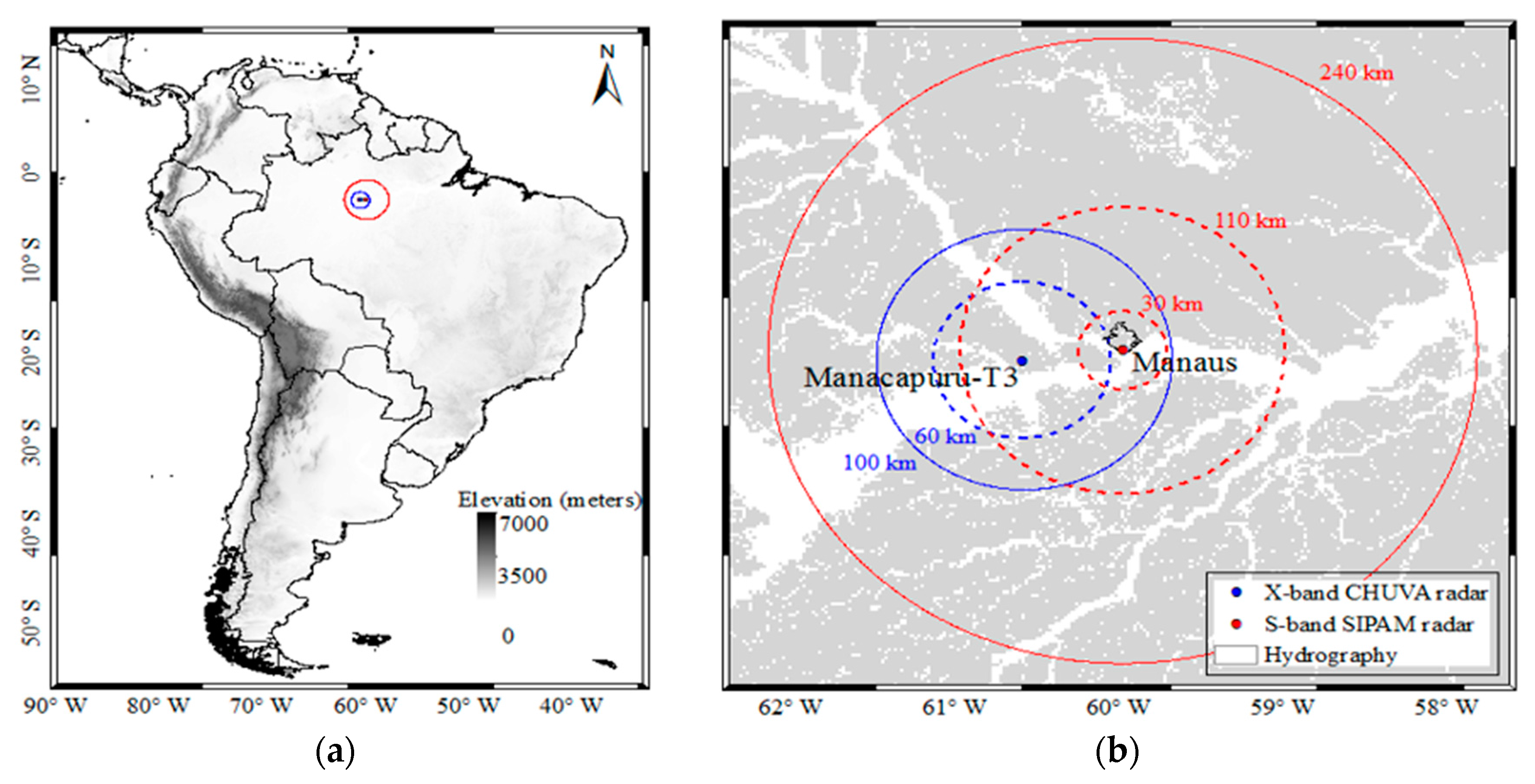
2.1. Study Area

This work focuses on an area in the middle of the Amazon basin, around the city of Manaus in the state of Amazonas, Brazil. The area covers a circle of 110 km in radius centered at 3.15°S and 59.99°W, where the S-band weather radar from the Amazon Protection National System (SIPAM) is located (Figure 1). The study period goes from March–September 2014, which includes part of the two GoAmazon/CHUVA Intensive Operating Periods (IOPs): IOP1 (wet season) from 1 February to 31 March 2014 and IOP2 (dry season) from 15 August to 15 October 2014 [22]. The Aerosol, Cloud, Precipitation, and Radiation Interactions and Dynamics of Convective Cloud Systems (ACRIDICON) campaign was also held during I0P2.
The precipitation pattern over the study region is closely linked to the South American monsoon system (SAMS [24,25,26]), which is related to several factors ranging from the local to the synoptic scale. The first factor is local convection, triggered by forest-pasture, river breeze, topography and the urban heat island affect [27,28,29]. Secondly, mesoscale factors, such as squall lines [30,31], although most frequent in the eastern portion of the Amazon basin, penetrate and propagate from the northeastern region to the center of the basin and produce synoptic convective events, which are most common and intense during wet-to-dry and dry-to-wet transitions. Thirdly, the synoptic scale Intertropical Convergence Zone (ITCZ) and the influence of biomass aerosol [32] are the major weather systems/conditions responsible for affecting the rainfall frequencies and intensities and cloud cover (lowest in July and August and highest in February and March). Thus, several precipitation systems and local factors are responsible for modulating the diurnal cycle of precipitation (often leading to late night or early morning precipitation in Manaus) and for controlling the wet-dry seasons in the region around Manaus [33,34].
According to Martin et al. [22], who used TRMM rainfall estimates (3B42_V7 product) from 2000–2014 over the Amazon basin, the 2014 wet season (IOP1) presented rainfall amounts greater than the fifteen-year mean (~200 mm) around Manaus, except over the southern region, which presented values between 100 and 150 mm less than the mean accumulated precipitation. On the other hand, spatially-distributed positive and negative anomalies of accumulated precipitation were observed around Manaus during the 2014 dry season (IOP2), when precipitation patterns are mainly associated with local characteristics.

2.2. Data Sources

Two GPM rainfall products, Level-3 IMERG and Level-2 GPROF2014, are evaluated over the central Brazilian Amazon, considering the S-band SIPAM weather radar in the city of Manaus as a reference. The S-band SIPAM is evaluated with respect to the X-band dual polarization weather radar from the CHUVA project (X-band CHUVA radar). A brief description of the datasets used in this study is provided next.

2.2.1. Radar Rainfall Estimates

The X-band CHUVA radar takes advantage of polarimetric variables for rainfall estimates based on the Dual Polarization Surface Rainfall Intensity (DPSRI) algorithm [35]. The DPSRI algorithm uses a combination of reflectivity (Z), specific differential propagation phase (Kdp) and rain rate (R) variables (a Z-Kdp-R relation), for X-band radars at a specific Constant Altitude Plan Position Indicator (CAPPI) level. A detailed description of the precipitation retrievals technique used by the X-band CHUVA radar and its performance in representing surface precipitation compared to rain gauges can be found in Gematronik [36] and Oliveira et al. [17].
The rainfall estimates from the SIPAM Manaus radar used in this study are processed by Texas A & M University. The rainfall estimates are obtained through the CAPPI product, based on the 240-km radial dataset. CAPPI products are available for 0.5–20 km of vertical level. The vertical and horizontal resolutions are 500 m and 2 km, respectively. In order to eliminate spurious data (e.g., noise, ground clutter) and improve the quality of the CAPPI products, a correction of the reflectivity field is performed. A calibration constant is applied to the CAPPI files during the following periods: from 9 February 2014 to 27 August 2014 (+2.0 dB), from 28 August 2014 to 16 October 2014 (−3.0 dB) and from 17 October 2014 to 17 August 2015 (−6.0 dB). The calibration constants are derived based on a comparison with TRMM PR data [37], providing the 56 dBZ baseline for IOP1, and a study of ground clutter pixels to determine the stability of the radar dataset [38]. Calibration is determined using base scan information from gridded Plan Position Indicator (PPI) scans.
The rainfall estimates are generated using the radar corrected reflectivity data at the 2.5-km CAPPI level within a radius of 160 km of coverage. A power law relation (Mismo relationship), which was found to be the most appropriate relation for GoAmazon based on comparisons with rain gauge measurements, is used for the conversion of radar reflectivity values to rain rates (Equation (1)):
Z = 178.0 R1.44
where Z is the horizontal reflectivity (in dBZ) and R is the radar rain rate (in mm·h−1). A final radar rainfall product with a spatial/temporal resolution of 2 km/10 min is then provided.

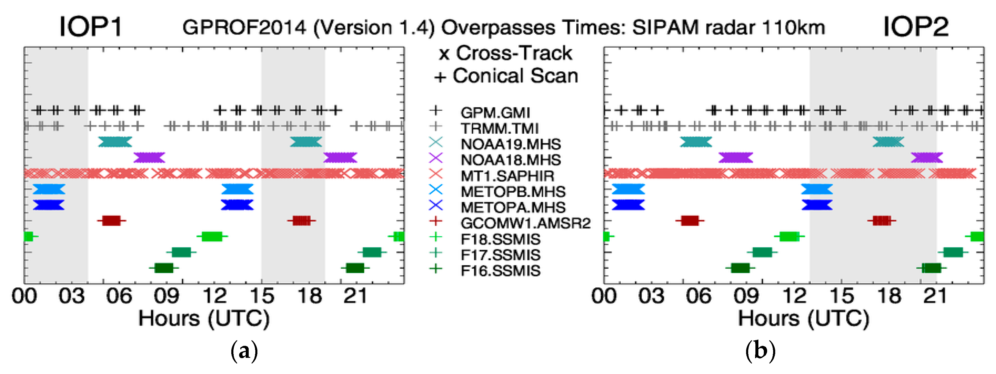
2.2.2. Goddard Profiling Algorithm

GPROF is a multichannel physical approach for retrieving both the instantaneous rain rate and the vertical structure information using PMW radiometers on board low-orbiting satellites. GPROF uses a Bayesian statistical approach to retrieve the vertical structure of precipitation over land and ocean and has been developed and enhanced for GPM. GPROF was originally developed for Special Sensor Microwave/Imager (SSM/I), but also applied to the TRMM Microwave Imager (TMI) using the 2A12 algorithm [39,40] and adapted for the Special Sensor Microwave Imager/Sounder (SSMI/S) for the F16, F17 and F18 satellites [41].
GPROF aims to retrieve the instantaneous rainfall rate and the rainfall vertical structure by using the response functions in different channels peaking at different depths within the raining column. According to Bayes’ theorem, the probability of a particular rain profile (R) given the brightness temperature vector (Tb) is defined as Equation (2):
Pr(R | Tb) = Pr(R) × Pr(Tb | R)
where Pr(R) is the probability with which a certain profile R is observed and derived using cloud-resolving models (CRM). The second term on the right-hand side of Equation (2), Pr(Tb | R), is the probability of observing Tb, given a particular rain profile R. This conditional probability is obtained using radiative transfer schemes to compute the brightness temperatures corresponding to the CRM output. Together, the radiative transfer and the convolution of these temperatures to the appropriate sensor resolution scheme comprise the forward modeling portion of the retrieval algorithm. In its current version (2014, Version 1.4), GPROF is applicable to different PMW sensors (imagers and sounders) and scan types (conical and cross-track), such as SSMI/S sensor on the DMSP(F16/F17/F18) satellites; Advanced Microwave Scanning Radiometer 2 (AMSR2) on board the Global Change Observation Mission-Water 1 (GCOMW1) satellite; GMI on board the GPM core observatory; TMI on TRMM satellite; Sondeur Atmosphérique du Profil d'Humidité Intertropicale par Radiométrie (SAPHIR) on Megha-Tropiques 1 (MT1); Microwave Humidity Sounder (MHS) on board the European Meteorological Operational A and B (METOP(A/B)) and the NOAA 18 and 19, as described by Kummerow et al. [42] and Kidd et al. [43]. The GPROF2014 algorithm Version 1.4, applied to the GPM database [44], is analyzed in this work. Table 1 lists some of the basic characteristics of the GPM constellation PMW sensors and the respective satellites that carry them.

2.2.3. Integrated Multi-SatellitE Retrievals for GPM

IMERG is a Level-3 algorithm that is intended to intercalibrate, merge and interpolate all available PMW estimates of the GPM constellation (e.g., GMI, TMI, SSMIS, AMSR2 and MHS), with PMW-calibrated IR estimates and gauge observations, to produce a quasi-global (60°N–S) 0.1° × 0.1° and 30-min dataset, from 1998 to the present [45,46].
Rainfall estimates, initially retrieved by the PMW sensors through the GPROF2014 algorithm, are combined and inter-calibrated with three prior multi-satellite algorithms: (i) TRMM Multi-satellite Precipitation Analysis (TMPA; [47,48,49]); (ii) Climate Prediction Center (CPC) Morphing-Kalman Filter Lagrangian time interpolation scheme (CMORPH-KF; [50,51]); and (iii) the Precipitation Estimation from Remotely Sensed Information using Artificial Neural Networks-Cloud Classification System re-calibration scheme (PERSIANN-CCS; [52]). In parallel, CPC assembles the zenith-angle-corrected, intercalibrated “even-odd” geo-IR fields and forwards them to Precipitation Processing System (PPS) for use in the CMORPH-KF Lagrangian time interpolation scheme and the PERSIANN-CCS computation routines. The PERSIANN-CCS estimates are computed (supported by an asynchronous re-calibration cycle) and sent to the CMORPH-KF Lagrangian time interpolation scheme. The CMORPH-KF Lagrangian time interpolation (supported by an asynchronous KF weights updating cycle) uses the PMW and IR estimates to create half-hourly estimates. Then, the IMERG ‘‘Final” run combines the interpolated observational precipitation data from the Global Precipitation Climatology Center (GPCC) Monitoring Product (currently Version 4). The Level-3 IMERG Final Run (research) product at 0.1° × 0.1° and half-hourly resolutions, from March–September 2014, is adopted in this study.

2.3. Evaluation Methods

2.3.1. Radar Rainfall Estimates as Reference

A validation analysis during March 2014 (CHUVA-GoAmazon, IOP1) is performed to assure that those S-band SIPAM radar retrievals accurately represent the instantaneous rain pattern observed over the region and can be used further for satellite evaluations. The S-band SIPAM radar evaluation is performed spatially (pixel-by-pixel), by comparison with the more accurate radar-based rainfall estimates by the X-band CHUVA radar. The comparison between X-band CHUVA and S-band SIPAM is performed over the X-band CHUVA radar coverage area (60-km radius).
Given the different spatial-temporal resolutions, the X-band CHUVA radar data are resampled from their native 200-m resolution to the S-band SIPAM 2-km spatial resolution. X-band CHUVA radar pixels are averaged within the S-band CHUVA radar pixel. A maximum time interval of 2 min between both datasets is considered. A minimum threshold is set to 0.2 mm·h−1, and 804 coincident time steps (cases) are analyzed, with a total of 2,173,212 grid points. The S-band SIPAM radar is chosen over the X-band CHUVA radar because of its longer record and larger area. The S-band SIPAM radar is an operational weather radar, which provides real-time monitoring. X-band CHUVA radar is only available during the specific IOPs, and it is limited up to 60 km due the attenuation effects.

2.3.2. Satellite-Radar Comparison

In order to evaluate the GPM satellite rainfall estimates over Manaus, IMERG and GPROF2014 are compared to the S-band SIPAM radar rainfall estimates, for coincident (spatial and temporal) points during the period from March–September 2014. A radar coverage area of 30–110 km in radius is adopted because of radar physical limitations in detecting signals directly above it (“cone of silence”) and far at the constant altitude of 2.5 km. A minimum threshold of 0.2 mm·h−1 for radar and satellite datasets is used. Considering that IMERG is a half-hourly precipitation product, with the precipitation being an average of all observations in the 30-min range, the S-band SIPAM radar estimates are integrated to the same temporal resolution. Such an integration criterion considers a minimum of 3 time steps of S-band SIPAM radar for a 30-min radar final product. For the GPROF2014-radar comparisons, the native (instantaneous) radar-rainfall estimates are used as a reference, and a maximum time interval of 5 min between those datasets is considered. Matching in space is performed by converting the S-band SIPAM radar to the satellite product grid. Given that the total rain amount, the rain area and/or the PDF shape can be affected by the resampling technique [53], the mean of the S-band SIPAM radar pixels inside the IMERG and GPROF2014 pixels is computed. Thereby, the original satellite rainfall estimates are preserved in their native spatial/temporal resolutions: (i) IMERG regular grid at 0.1° × 0.1° half-hourly; and (ii) GPROF2014 satellite projection (conical and cross-track) with a spatial resolution varying depending on the sensor (Table 1) and up to two sampling overpasses per day in a given region. The total number of cases and samples for each product is shown in Table 2.

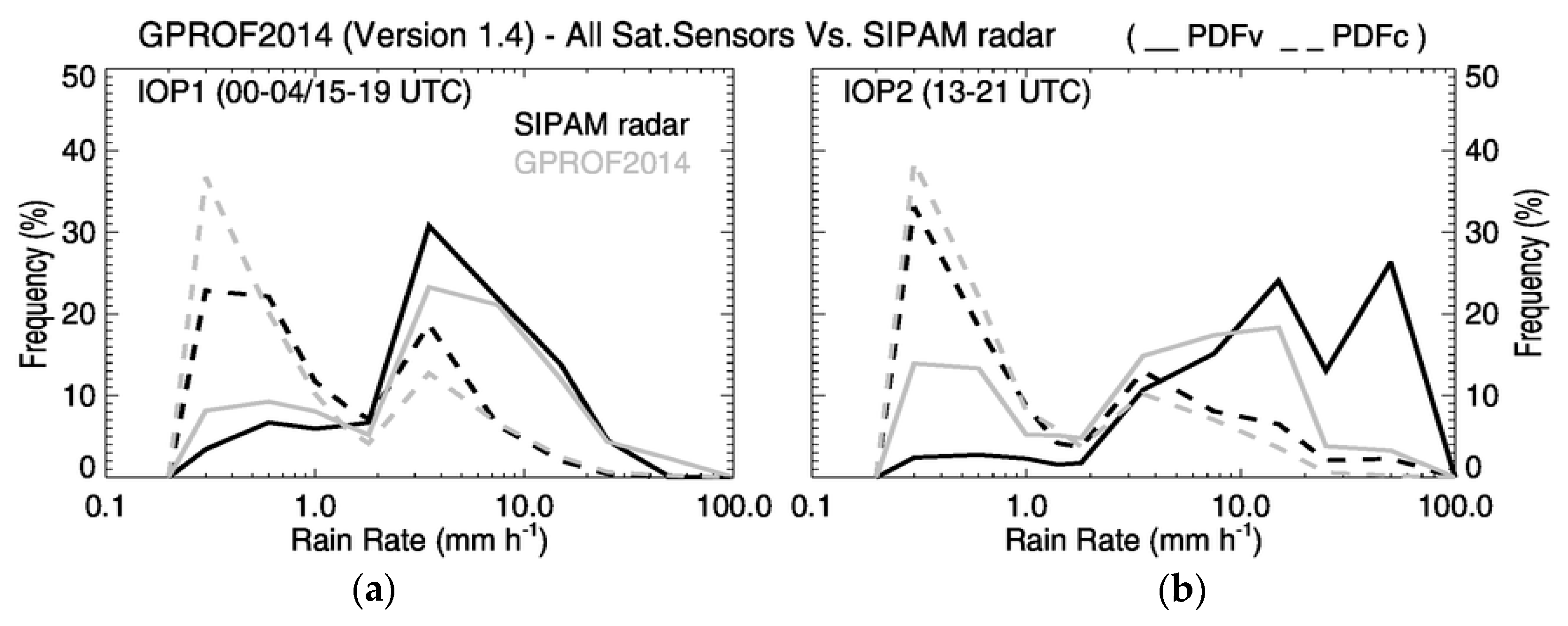
2.3.3. Probability Distributions by Rainfall Volumes and Occurrences

In order to study the satellite precipitation error distributions, we looked at volumetric (PDFv) and occurrence (PDFc) probability density function analyses [15,16,17,18,53]. The PDFv represents the relative contribution of each rain rate bin to the total rainfall volume. Similarly, the PDFc provides the frequency occurrences of each rain rate bin to the total number of occurrences. PDFc normally tends to emphasize lighter rainfall rates, due its high frequency of occurrence. We consider the following precipitation classes: 0.2–0.4, 0.4–0.8, 0.8–1.2, 1.2–1.6, 1.6–2, 2–5, 5–10, 10–20, 20–30 and ≥30 (in mm·h−1). The analysis is performed monthly from March–September and hourly for both wet (IOP1) and dry (IOP2) seasons over the S-band SIPAM radar coverage.

2.3.4. Statistical Analysis

The performance of satellite-based precipitation estimates is evaluated based on continuous and categorical statistical metrics [54,55]. To quantify the error between the estimate (A) and the reference (B) and their linear agreement, the following continuous verification statistics are investigated: correlation coefficient (COR), mean error (bias), root mean square error (RMSE) and standard deviation (SD). On the other hand, the categorical statistical scores include: (i) the probability of detection (POD), which measures the fraction of precipitation events that are correctly detected by A; (ii) the false alarm ratio (FAR), which gives the fraction of events that were misinterpreted as events; (iii) the success ratio (SR), which is the ratio of hits to the total number of estimated events; (iv) the critical success index (CSI) that measures the fraction of all estimated events that were correctly diagnosed; (v) and the bias score (BIAS), which gives the ratio of the estimated/observed rain pixels [56,57]. For both the continuous and categorical analyses, a minimum threshold of 0.2 mm·h−1 for A-B pairs is considered.
Continuous and categorical analyses can be graphically consolidated into the Taylor [58] and performance [59] diagrams. The Taylor diagram provides a way to summarize how closely a set of patterns matches observations, using COR, RMSE and SD. In Taylor diagrams, the SD increases with the radial distance from the origin and is normalized by the reference datasets, where 1.0 is the best reference value. In this performance analysis, bias values are also included in the Taylor diagram. The performance diagram utilizes the geometric relationship between SR, POD, BIAS and the CSI to display all four metrics simultaneously, with a perfect forecast lying in the upper right region of the diagram.

3. Results and Discussion

In this section, we present and discuss the performance of IMERG and GPROF2014 rainfall algorithms over the Manaus region in the Brazilian Amazon, using the S-band SIPAM radar as a reference. To ensure that the S-band SIPAM radar retrievals accurately represent the instantaneous rain pattern observed over the region, a comparison with the X-band CHUVA radar is performed in Section 3.1. The abilities of GPM IMERG and GPROF2014 to reproduce general precipitation characteristics and rainfall diurnal cycles are both analyzed with respect to the S-band SIPAM radar from March–September 2014.

3.1. How Good Is Our Reference for Evaluating Satellite Precipitation Products?

Figure 2 depicts a density scatterplot of the rain rate for S-band SIPAM radar against the X-band CHUVA radar (coincident area within a 60-km radius of the X-band CHUVA radar location). The corresponding PDFs and cumulative density function (CDFs), both in terms of volumes and occurrences, are also shown for March 2014. X-band CHUVA and S-band SIPAM radars show similar distribution patterns. COR, BIAS, RMS, POD and FAR recorded values of 0.7, 0.03 mm·h−1, 0.71 mm·h−1, 0.75 and 0.38, respectively.
The S-band SIPAM radar presents a slight overestimation of precipitation, mainly for light intensities (between 0.2 and 1 mm·h−1), which are the most frequent, i.e., high occurrence density (~45%). On the other hand, an underestimation of heavy rainfall volumes (greater than 10 mm·h−1) is observed. In terms of CDF distributions, about 76% and 80% of CHUVA and SIPAM rainfall occurrences are from rain intensity <1.0 mm·h−1 and 96% and 98% from rain intensity <10 mm·h−1. In terms of volumes, about 20% and 25% (70% and 78%) for rain intensity <1 mm·h−1 (<10 mm·h−1) are observed by CHUVA and SIPAM radars. These results demonstrate a good agreement between S-band SIPAM and X-band CHUVA radars, especially for the more frequent light events. The maximum differences in cumulative frequency between SIPAM and CHUVA occurrence and volume distributions are about 4% from light rain (<5 mm·h−1).
In summary, the S-band SIPAM radar shows similar rainfall patterns when compared to the X-band CHUVA radar in terms of PDF/CDF of rain occurrence and volume and is therefore considered suitable to use as a reference for evaluating satellite precipitation products. Specifically, light to heavy rainfall volumes and occurrences are well represented by S-band SIPAM, even though a slight overestimation in the frequency of light rainfall volume/occurrence and an underestimation of heavy rainfall volumes are observed. Such behavior might be related to the fact that S-band SIPAM radar retrieval assumes a constant particle size distribution (see Equation (1)), which may cause a misinterpretation of the correct drop size distribution (DSD) and, consequently, a better quantification of instantaneous rain rate. However, the general pattern of rainfall distribution proved to be consistent in representing the maximum frequencies of occurrence and volume over distinct rainfall classes. A good alternative to investigate this effect is the assumption of more appropriate Z-R relationships for SIPAM rainfall retrievals. Although the X-band CHUVA radar is resampled to the same resolution of S-band SIPAM radar (2 km × 2 km), the accurate physical capability of the X-band radar in capturing smaller and more intense rain cells is limited over distances where attenuation is not major [60].

3.2. Assessment of GPM-Based Products

Figure 3 summarizes the monthly performances of IMERG relative to the S-band SIPAM radar, through continuous and categorical analyses using Taylor and performance diagrams over the Manaus region for March–September 2014. Both Taylor and performance diagrams show a seasonal dependence, which is strongly linked to the precipitation regime in the region. The Taylor diagram, which uses a combination of COR, SD, RMSE and bias parameters to represent the performance of the product compared to the reference, shows an under-performance of IMERG during all months (Figure 3a). A slight wet-to-dry influence in monthly COR is noted, with values ranging from 0.1 (dry) to 0.4 (wet). This wet-to-dry dependence is even more evident in the RMSE, SD and bias, which vary from 1.0 to 2.0, 0.0–2.0, and −0.18–0.15 mm·h−1, respectively, going from the wet to the dry season. The wetter (drier) months show higher (lower) RMSE and SD and positive (negative) bias. In the performance diagram, optimal values of SR, POD, BIAS and CSI score combinations lie in the upper right region (Figure 3b). The wetter months present the highest CSI and the lowest FAR compared to drier months, which implies better categorical performance during the wet months, compared to the drier months.
Figure 4 depicts monthly PDFs (both PDFv and PDFc) analysis for S-band SIPAM radar and IMERG during March–September 2014. Overall, for both rainfall products, volumes between 5 and 20 mm·h−1 largely contribute to the total rainfall accumulated during the study period, representing about 20%–35% of the total monthly rainfall. In terms of precipitation occurrences, the largest relative contribution is provided by light rains (<1 mm·h−1) at around 35%, with events between 2 and 5 mm·h−1 also largely contributing (~20%) to the total number of events. Distinct seasonal characteristics are also observed over the Manaus region, especially in the heavy rainfall classes (i.e., >20 mm·h−1). Drier months are mainly characterized by volumes of rains above 20 mm·h−1, whereas wetter months are characterized mainly by events between 5 and 10 mm·h−1. The frequency of light (0.2–0.4 mm·h−1) and heavy (i.e., >20 mm·h−1) rainfall increases from March–September, while an opposite behavior is observed for moderate rainfall (2–5 mm·h−1) occurrences.
The shift in heavy rain frequency from wet to dry periods can be explained by the increasing thermodynamic forcing, such as a reduction in the inversion layer and an increase in the convective available potential energy (CAPE) and moisture [33], which characterizes local and intense convective rain cells in the region. During the wet season, besides higher rainfall amounts influenced by the SAMS life cycle [26], rain volumes and occurrences are also linked to synoptic/large-scale precipitating systems, e.g., squall lines [30]. Thus, the interaction of systems from local to large scales and from wet to dry periods strongly influences the amounts and occurrences of rainfall, through the modulation of the diurnal cycle of precipitation.
As shown in Figure 4, IMERG presents an opposite pattern in PDFv and PDFc distributions compared to S-band SIPAM radar, mainly at moderate and heavy rain rates. During the wet season, IMERG tends to overestimate volumes of moderate and heavy rain rates (>10 mm·h−1). On the other hand, an underestimation in the volume frequency of moderate and heavy rainfall classes is observed during the dry period, which is compensated by an overestimation in the frequency of light to moderate rainfall (1–10 mm·h−1) volumes. Moreover, IMERG tends to sample less light rain rates than the radar (<1 mm·h−1 for the wet season and 0.2–0.4 mm·h−1 for the dry season), showing poor detection of light rain rates (<0.4 mm·h−1) and overestimating the 0.4–10 mm·h−1 rainfall occurrences. The wet-dry divergence in the IMERG ability of quantifying (PDFv) and detecting (PDFc) heavy rainfall events may be attributed to: (i) PMW rainfall incursions through the GPROF2014 algorithm; (ii) physical principles associated with the rainfall inference through the IR channel, which relates the cloud top brightness temperatures to the surface rain rate; (iii) errors in the integration among the different retrieval algorithms (i.e., TMPA, CMORPH-KF and PERSIANN-CCS) that generate the IMERG dataset; and/or (iv) bias adjustment with the GPCC observational data usage.

3.3. Precipitation Diurnal and Seasonal Cycles

In this section, we evaluate IMERG’s ability in reproducing the diurnal cycle against the S-band SIPAM radar. Figure 5a investigates the rain diurnal cycle by looking at the mean and standard deviation (SD) of rain rates for the IOP1 (wet) and IOP2 (dry) periods by the S-band SIPAM radar. Both periods present high rain rates during daytime, which is related to the thermodynamic conditions in the region. During the wet period, the S-band SIPAM radar mean rainfall presents a primary peak of 0.6 mm·h−1 around 10:00–13:00 UTC, where maximum values of SD (2 mm·h−1) are also observed. A secondary SD peak (1.6 mm·h−1) at around 00:00 UTC is observed, which might be related to organized mesoscale convective systems over the region.
In the dry period, the S-band SIPAM radar presents peaks of rain rate mean and SD between 15:00 and 21:00 UTC, with values around 1 and 4.5 mm·h−1, respectively. Secondary rainfall mean (~0.4 mm·h−1) and SD (~1.8 mm·h−1) peaks are found in the first hours of the day (from 00:00–08:00 UTC). The dry period is also characterized by higher SD than the wet period, which suggests a larger spatial variability of rainy events. During the dry period, local characteristics are more evident, and preferential occurrence locations of convective rain cells are driven by local surface types and thermodynamic conditions [32], which explain the reason for the high mean and SD differences between IOP2 and IOP1.
The S-band SIPAM radar mean values and peak hours during the wet (dry) period at 10:00–13:00 UTC (15:00–21:00 UTC) over the Manaus region corroborate the results by Tota et al., Angelis et al., Machado et al. and Tanaka et al. [29,33,34,61]. Tota et al. [61] attributed the maximum frequency around 19:00 UTC (15:00 Local Time) during the dry season to isolated convective activity and the secondary (around 08:00 UTC) to organized mesoscale convective systems. Angelis et al., Machado et al. and Tanaka et al. [29,33,34] showed that rainfall frequencies and intensities vary over the study region and that primary peaks may change according to surface type (forest, city, among others).
Figure 5b shows box plots of rain rate differences (in mm·h−1) between IMERG and S-band SIPAM radar observations. During the wet season, IMERG presents reasonable agreement with the reference, especially during the peak hour times (between 10:00 and 13:00 UTC), with the median differences close to 0 mm·h−1, 25th and 75th varying from −1 and 1 mm·h−1 and minimum and maximum values varying from −4 and 4 mm·h−1. IMERG shows an overestimation between 00:00–04:00 UTC and 15:00–18:00 UTC, especially at 03:00 UTC, which presents the highest values of SD (12 mm·h−1). On the other hand, IMERG fails to reproduce the diurnal cycle structure during the dry season, showing an underestimation of hourly rainfall and a poor representation of hourly peaks between 13:00 and 21:00 UTC. The IMERG-SIPAM maximum negative differences during the dry period are observed at 18:00 UTC. At this time, which corresponds to the maximum values of rainfall mean and SD observed by the SIPAM radar, large error bounds are observed, which suggests that IMERG is not able to detect the large spatial variability of rainy events in the region.
Figure 6 and Figure 7, similarly to Figure 4, show the PDFv and PDFc distributions, but at the hourly scale and focused on IOP1 and IOP2, respectively. The diurnal cycle main pattern observed by the S-band SIPAM radar reveals distinct PDFv and PDFc distributions between the two periods. During the wet period (Figure 6), the rainfall between 5 and 20 mm·h−1 shows high frequency (~40% of the total volume). A slight contribution of heavy rainfall (>20 mm·h−1), around 00:00 and 12:00 UTC, in terms of both volumes and occurrences is also observed. During the dry period (Figure 7), the contribution of moderate and heavy rainfall (>5 mm·h−1) volumes/occurrences is more homogeneous than during the wet period. The occurrence of light rain rates is more frequent (>50%) in the dry period than in the wet period, except for 15:00–21:00 UTC, when the occurrence of heavy rain shows high frequencies.
IMERG and the S-band SIPAM radar present similar distribution patterns, with high frequencies (around 40%) of rainfall volumes between 5 and 20·mm h−1. However, IMERG tends to underestimate hourly light precipitation intensities and frequencies (between 0.2 and 0.4 mm·h−1). This corroborates what was observed by Tang et al. [61] over five distinct regions of Mainland China. The positive (negative) biases during the wet (dry) period are mainly due to the overestimation (underestimation) of heavy rainfall volumes. In the wet period, overestimation (~20%) of heavy rainfall (>20 mm·h−1) volumes (PDFv) is observed especially at 00:00–03:00 and 15:00–21:00 UTC, clearly not related to the peak hours observed by the S-band SIPAM radar. In the dry period, the underestimation of rain volume (~40%) of rainfall greater than 10 mm·h−1 is recorded during the peak hours, between 13:00 and 21:00 UTC.
IMERG performance dependence on seasonal and diurnal cycles is particularly evident when the contribution from different rainfall classes is analyzed. During the wet season, precipitation in the Central Amazon is mainly dominated by large-scale systems (e.g., ITCZ and squall lines) and contributes with high frequency of relatively moderate rainfall (~5 mm·h−1) at any time of the day. IMERG shows a frequency overestimation during the non-peak hours, which suggests a systematic error. On the other hand, in the dry period, which presents more convective patterns that are concentrated around 18:00 UTC, IMERG shows an underestimation. This may be due to the satellite capability (e.g., spatial resolution) in detecting the presence of intense and localized convective rain cells.

3.4. Investigation on Possible Sources of Inaccuracy

In order to investigate the source of IMERG inconsistencies in reproducing the rainfall diurnal cycle, an evaluation of GPROF2014 over the Manaus region is performed. Figure 8 shows the hourly overpasses of eleven satellite/sensors (conically and cross-track scanning) in the GPM constellation and used in the GPROF2014 rainfall retrievals over the S-band SIPAM radar coverage during IOP1 and IOP2. Figure 8 also shows the times at which IMERG overestimates and underestimates the reference rain rates (shown in Figure 5, Figure 6 and Figure 7). Conical and cross-track PMW satellite sensors have a quasi-total daily coverage, with certain preferential hour times by each satellite/sensor at specific times. For example, during the IOP1 and IOP2 (shaded areas), the retrievals are based on the following sensors: SSMI/S from F16 (for IOP2) and F18 (IOP1) satellites; AMSR2 (GCOMW1 satellite); MHS from the METOPA, METOPB, NOAA18 (only in IOP2) and NOAA19 satellites; SAPHIR (MT1); and TMI and GMI from the TRMM and GPM satellites.
Figure 9 depicts the mean characteristics observed through PDFv and PDFc analysis from all of the GPROF2014 sensor/satellite overpasses against its coincident S-band SIPAM radar time steps at 00:00–04:00 and 15:00–19:00 UTC, during IOP1, and 13:00–21:00 UTC (IOP2). Overall, GPROF2014 has a good performance in terms of PDFv and PDFc when compared to S-band SIPAM radar measurements. However, GPROF2014 slightly overestimates the volume and occurrence of light (<1 mm·h−1) and heavy (>30 mm·h−1) rainfall and underestimates moderate rain (around 2 and 10 mm·h−1) at 00:00–04:00 and 15:00–19:00 UTC during IOP1. During IOP2 (13:00–21:00 UTC), when a convective PDFv distribution pattern is expected, GPROF2014 strongly underestimates the frequency of heavy rainfall (>20 mm·h−1) volumes, up to 20% less than those observed by S-band SIPAM radar. For light rainfall (<1 mm·h−1), GPROF2014 shows an overestimation in terms of volume (~10%), but good agreement with S-band SIPAM radar in terms of occurrences (i.e., PDFc distribution).
The physical characteristics of GPROF2014 PMW rainfall retrievals (e.g., sensor-based spatial resolution, representation of hydrometeors profiles, among others) may be indicated as the main cause of the algorithm limitations. In addition, the surface type factor (i.e., land, ocean, inland water, among others) and their different emissivity signals may also have significant contributions in adopting a particular hydrometeor profile and consequently in the final rainfall retrieval product. Figure 10 shows the GPROF2014 original-overland differences, which emphasize the portion of precipitation over the inland water (along the Negro, Solimões and Amazon rivers, near Manaus, Amazonia, Brazil). Figure 10 presents differences between each sensor and the S-band SIPAM radar during those times in which IMERG performs poorly. The most prominent GPROF2014 original-overland differences are found during the GPM GMI satellite sensor overpasses. GPROF2014 GMI presents large overestimation (underestimation) of rain rate volume and occurrence greater (less) than 10 mm·h−1 up to 15%, during IOP1. Large overestimations around 13% in PDFv and ~15% in PDFc of rain rates between 5 and 10 mm·h−1 are observed on IOP2. However, an underestimation of light rain rate occurrence frequency is observed by GPROF2014 for the GMI sensor. Evidence of the influence of the Amazon River and the topography in local circulations, cloud cover and, consequently, precipitation in the region, are well reported by observational data, such as radar and rain gauge and also by satellites, e.g., [28,29,32,33,62]. However, such differences in IMERG, for both the wet and dry periods, appear more prominent due to some systematic errors, which can emerge from a non-suitable adjustment linked to the continent-ocean surface type adoption by the GPROF2014 algorithm for GMI sensor.

4. Conclusions

In this study, the IMERG (V03D, “final” run) precipitation product is evaluated against the S-band SIPAM radar in the proximity of Manaus city, located in the Brazilian Amazon region. The analysis is performed during two seasons (wet and dry) from March–September 2014. Special attention is given to the March and September months (i.e., IOP1 and IOP2), when the GoAmazon and the CHUVA-ACRIDICON field campaigns took place. To better assess the limitations of IMERG in estimating the diurnal cycle of precipitation, during wet and dry periods, the GPROF2014 PMW rainfall estimates are also analyzed, especially during times when IMERG was not able to correctly quantify and/or detect rainfall.
The main conclusions of this work are:
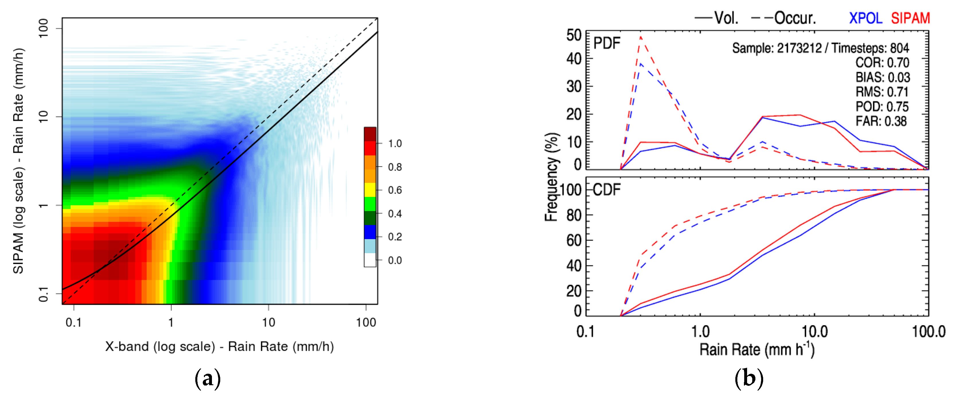
  • As an important initial step for further satellite precipitation validation analysis, S-band-SIPAM radar rainfall estimates are validated against another radar-based precipitation (i.e., the X-band dual polarization radar from the CHUVA project). Although a slight overestimation of light rainfall and an underestimation of heavy rainfall are observed in the PDFv and PDFc analysis, SIPAM radar is considered suitable to use as a reference dataset for validating satellite precipitation products.
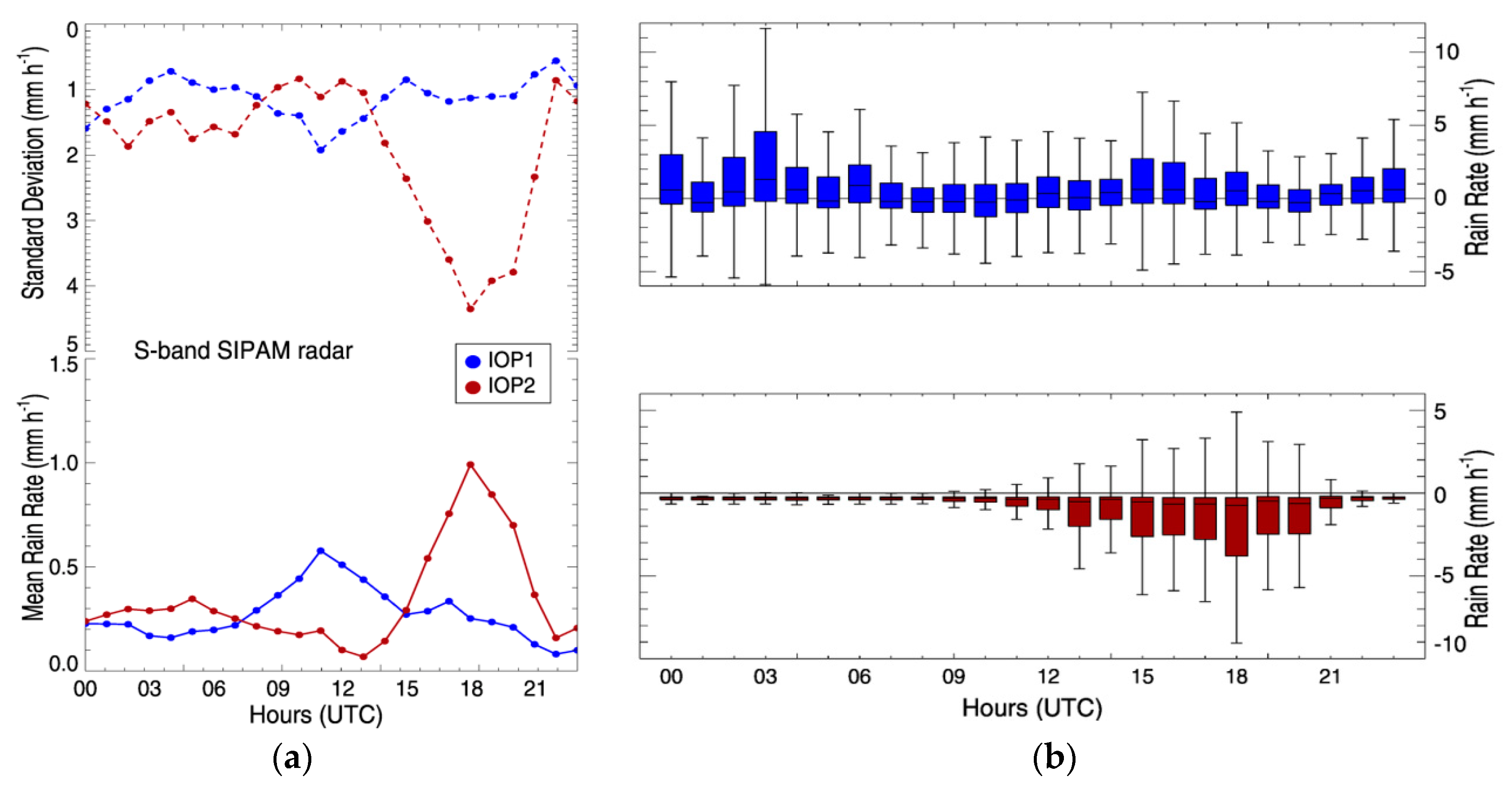
  • S-band SIPAM radar analyses revealed significant wet to dry contrast characteristics over the Manaus region by PDFv and PDFc distributions. During the wetter (drier) period, the volume and occurrence contributions of moderate (heavy) rainfall are clearly identified and strongly modulated by the diurnal cycle of precipitation.
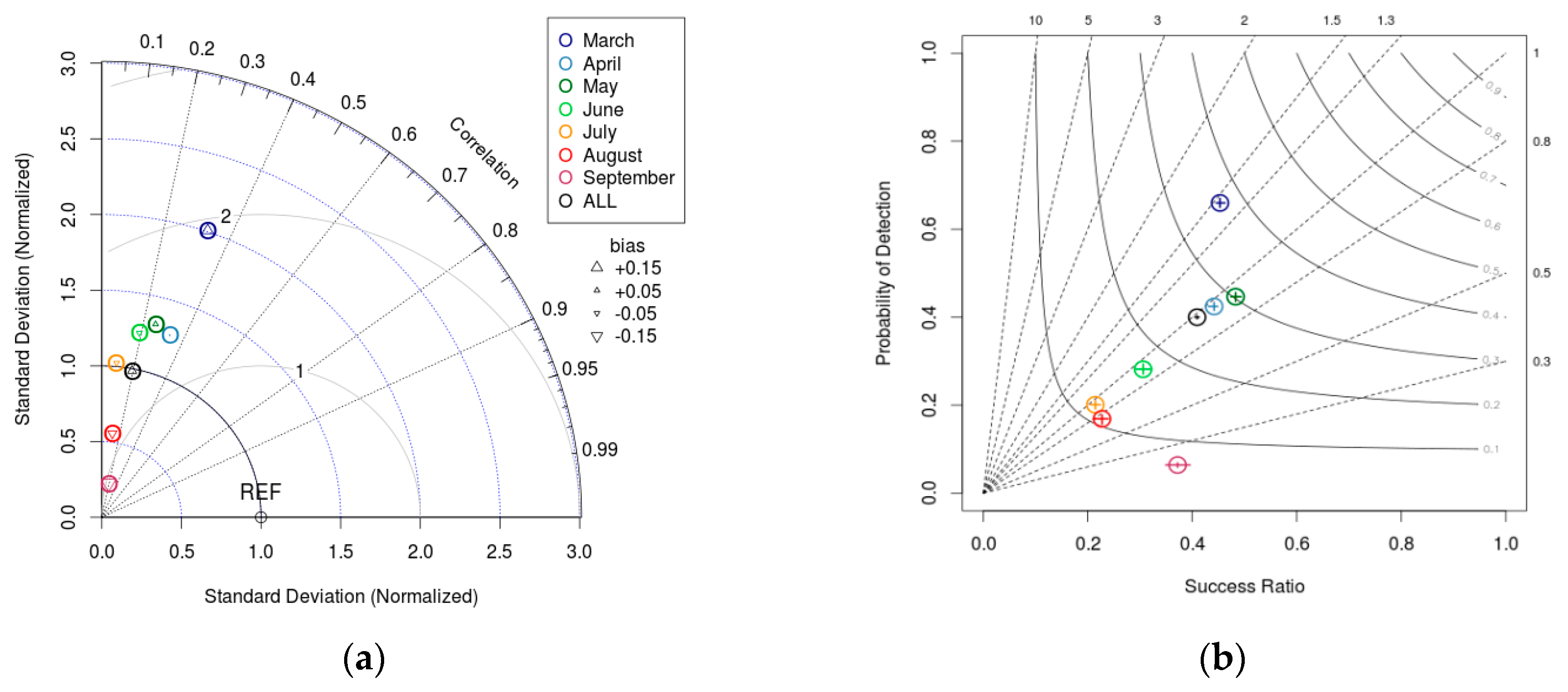
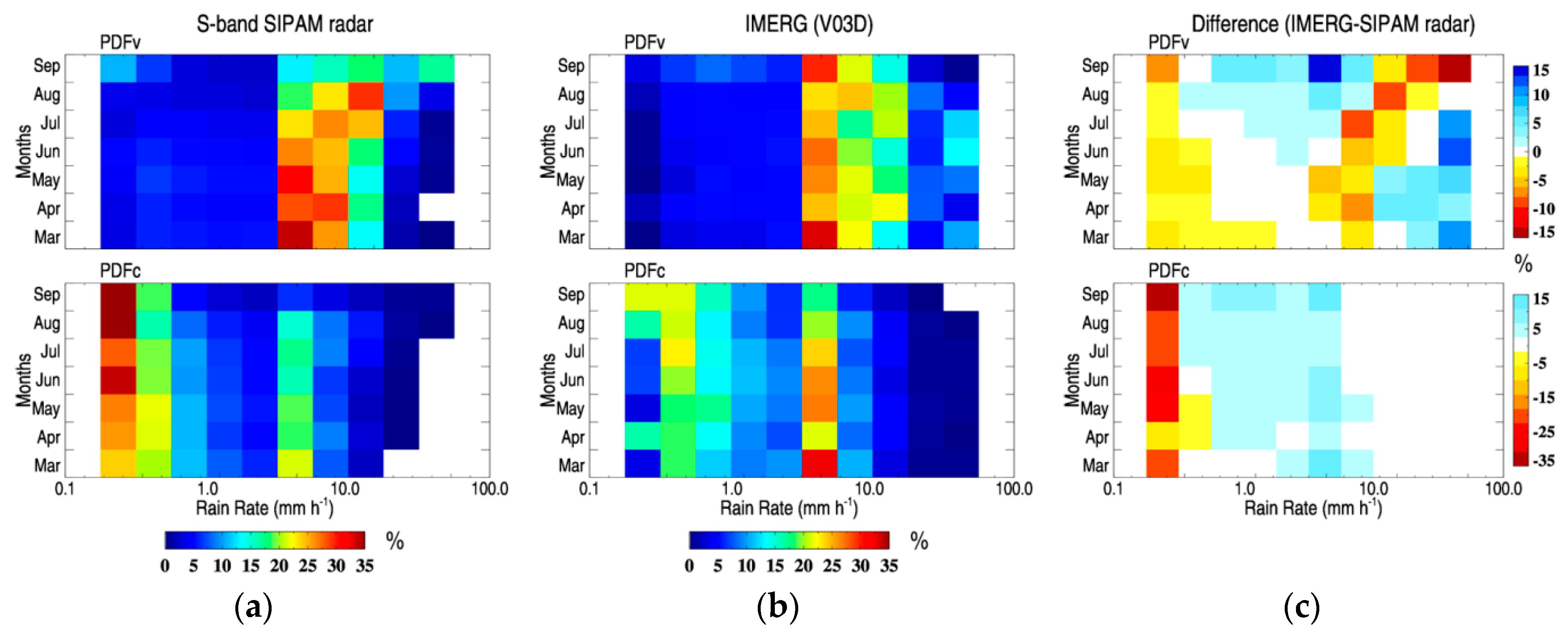
  • Statistical pixel-by-pixel analyses revealed a strong dependence of the IMERG dataset performance on seasonality. The Taylor and performance diagrams indicate that IMERG performances are strictly linked to the monsoonal rainfall pattern over the region. The overestimation (underestimation) of rain volumes is particularly significant for heavy rainfall classes (>10 mm·h−1) during IOP1 (IOP2).
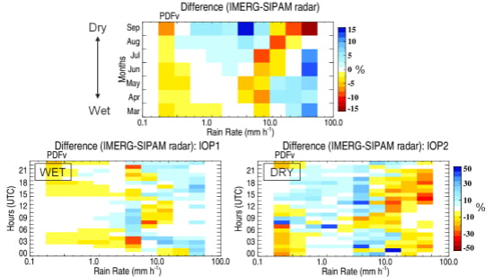
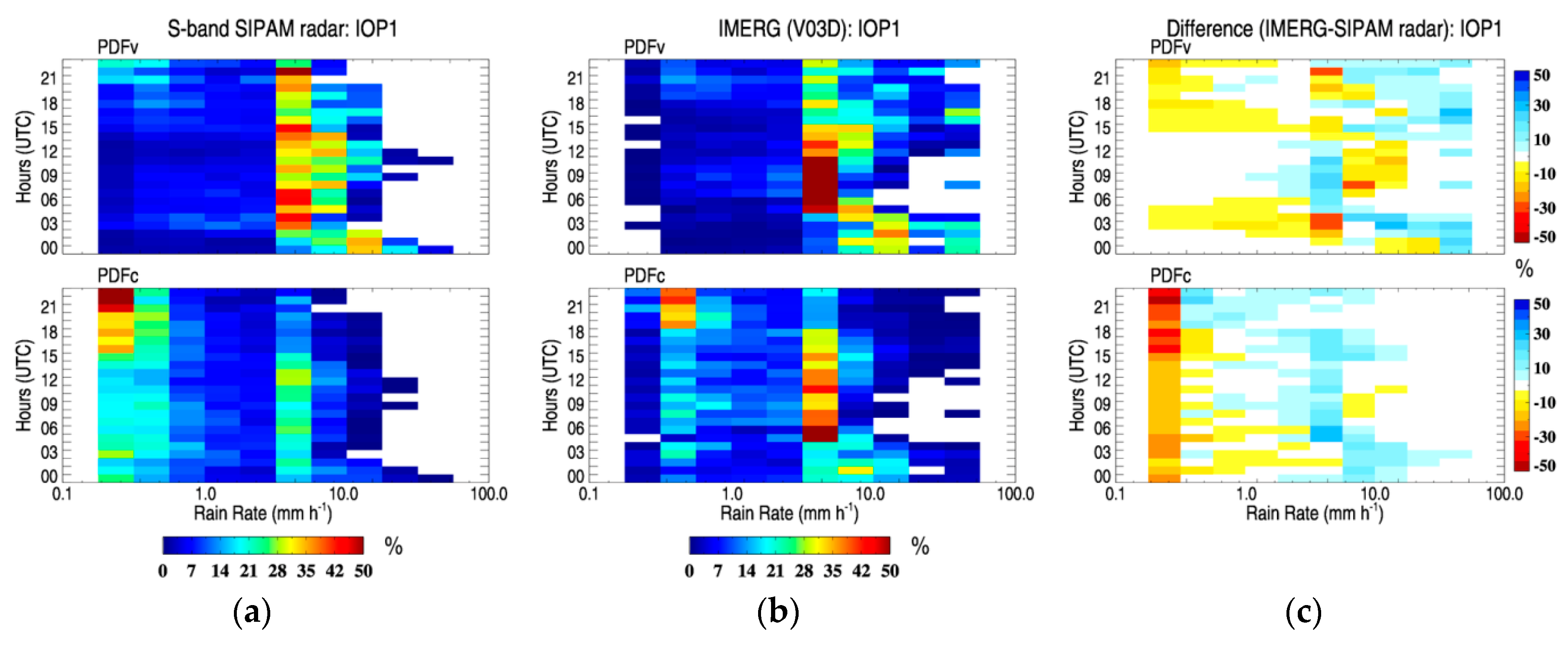
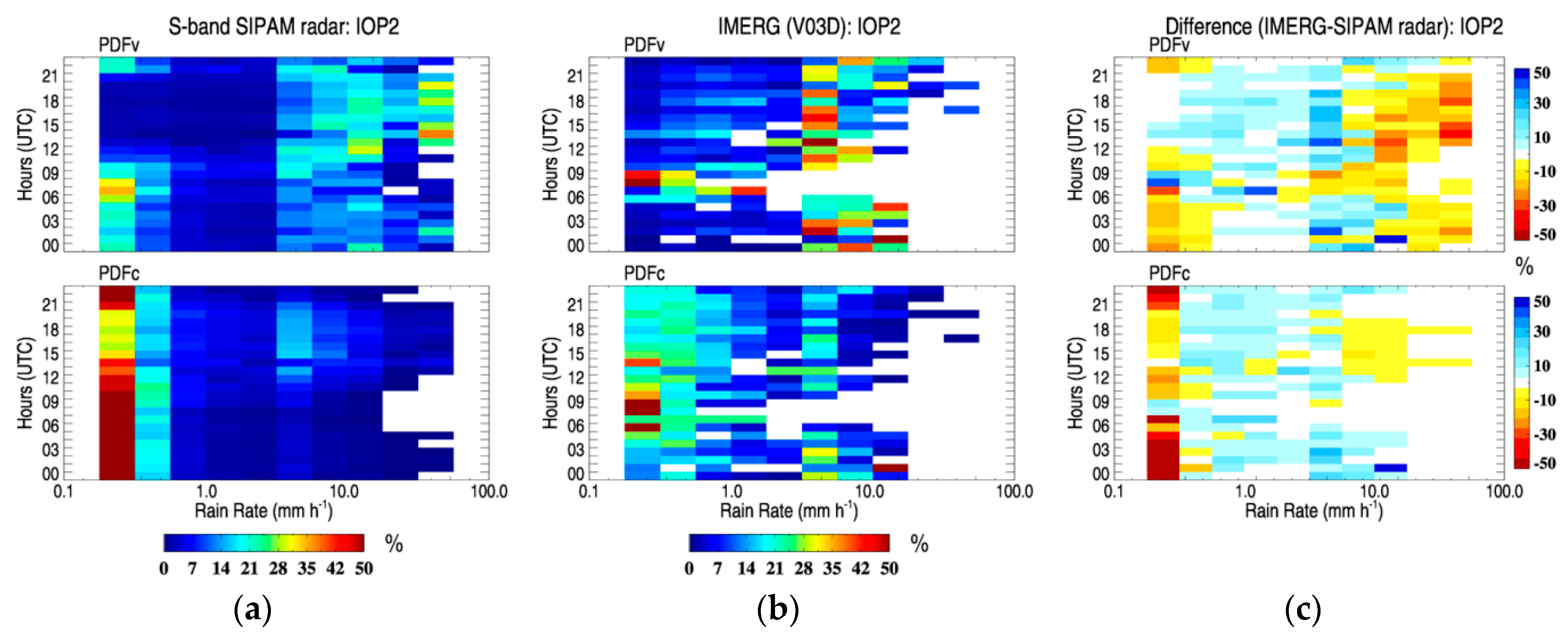
  • The diurnal cycle analysis during wet and dry periods presented certain times with strong discrepancies between IMERG and the reference. During IOP1, an overestimation between 00:00–04:00 UTC and 15:00–18:00 UTC is observed, due to an overestimation of the occurrence and volume of heavy rainfall. During IOP2, an opposite behavior with strong rainfall volume and occurrence underestimation is found at 13:00–21:00 UTC, mainly due to the non-captured isolated convective rain cells in the afternoon.
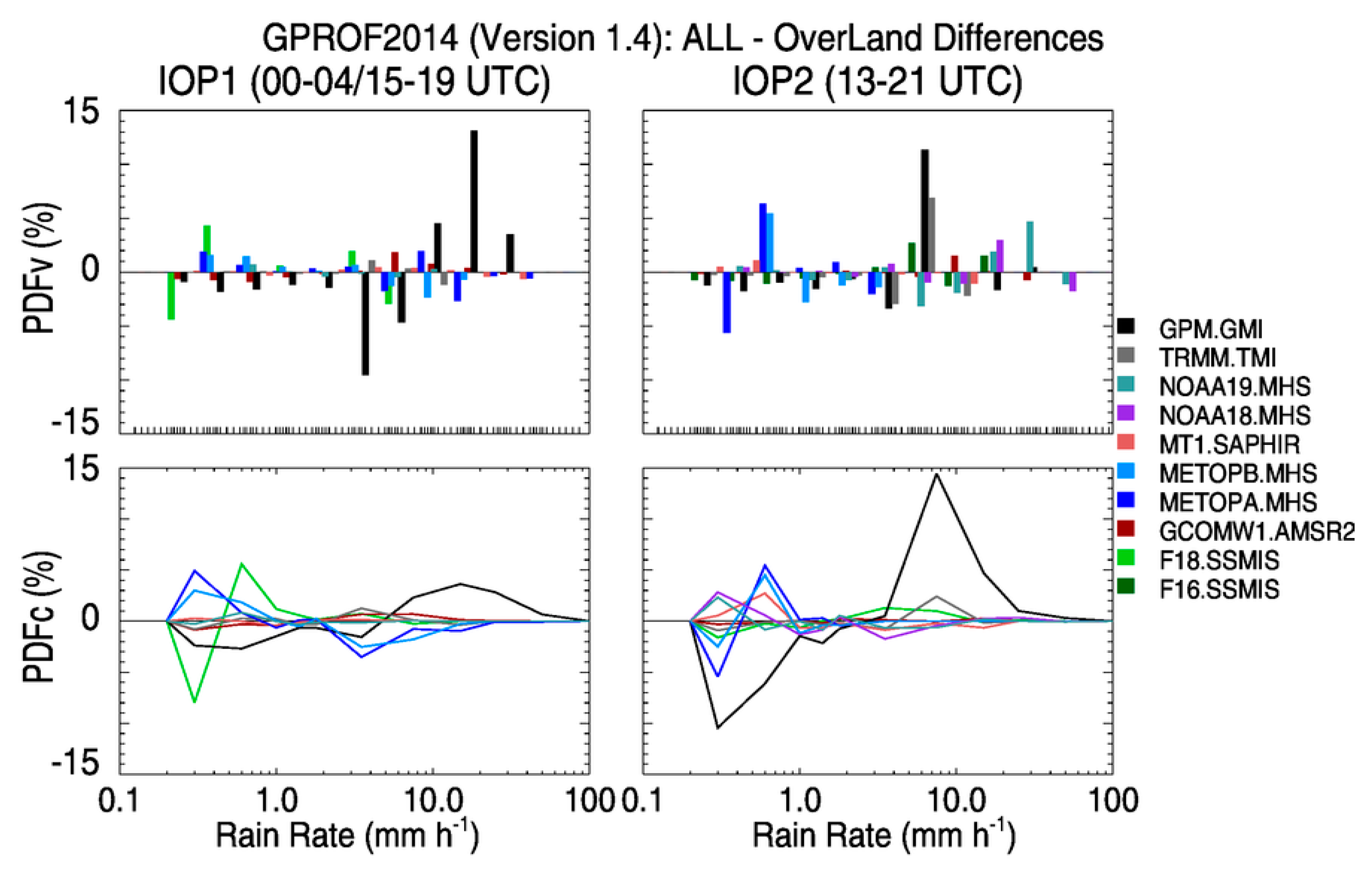
  • Analysis of the GPROF2014 algorithm rainfall sensor retrievals explains the IMERG’s poor performance. GPROF2014 slightly overestimates and strongly underestimates heavy rainfall volume and occurrence, during the IOP1 and IOP2, respectively. GPROF2014 for the GMI sensor rainfall retrievals presented the largest impact by inland water surface type, compared to other sensors. Thus, a significant portion of rainfall volumes and occurrences, observed by IMERG, comes from the GPROF2014-GMI rainfall retrievals, most prominent over the inland water surface type, along the Negro, Solimões and Amazon rivers.
This study revealed important information regarding the IMERG and GPROF2014 quality and limitations over the Central Amazon region. This issue was observed along the Negro, Solimões and Amazon rivers, but other regions of the globe and surface types should be deeply investigated. Our findings are critical for the correct and successful applications of GPM rainfall estimates for applications, like natural disasters monitoring, data assimilation systems, hydrological modeling, climatic studies and for better understanding the physical processes of precipitating systems over the region. These analyses also contribute to meliorating the GPM algorithm. Future studies should be directed to investigating the characteristics and distributions of uncertainties (systematic and random error components) for both GPROF2014 and IMERG satellite rainfall estimates and exploring other regions in Brazil and beyond.

Acknowledgments

The first author acknowledges the financial support of the National Council for Scientific and Technological Development (CNPq) and the Coordination for the Improvement of Higher Education Personnel (CAPES) Brazil during his PhD studies and also the Institutional Program of Overseas Sandwich Doctorate (PDSE) from CAPES (process 6836-15-1) for the internship opportunity. The author also thanks the Civil, Environmental and Infrastructure Engineering department at George Mason University for the infrastructure required for the development of this research. The authors acknowledge the CHUVA Project (FAPESP Grant 2009/15235-8), the Amazon Protection National System (SIPAM), Texas A & M University and NASA/Goddard Space Flight Center’s Mesoscale Atmospheric Processes Laboratory and PPS for the high-quality data provided for this study. The authors’ great gratitude is extended to Aaron Funk, Courtney Schumacher and Thiago Biscaro for the radar data support.

Author Contributions

Rômulo A. J. Oliveira designed the study, conducted the analysis and wrote the manuscript. Viviana Maggioni, Daniel A. Vila and Carlos A. Morales contributed to discussions and revisions, providing important feedback and suggestions.

Conflicts of Interest

The authors declare no conflict of interest.

References

  1. Kummerow, C.; Barnes, W.; Kozu, T.; Shiue, J.; Simpson, J. The Tropical Rainfall Measuring Mission (TRMM) sensor package. J. Atmos. Ocean. Technol. 1998, 15, 809–817. [Google Scholar] [CrossRef]
  2. Hou, A.Y.; Kakar, R.K.; Neeck, S.; Azarbarzin, A.A.; Kummerow, C.D.; Kojima, M.; Oki, R.; Nakamura, K.; Iguchi, T. The Global Precipitation Measurement Mission. Bull. Am. Meteorol. Soc. 2014, 95, 701–722. [Google Scholar] [CrossRef]
  3. Levizzani, V.; Bauer, P.; Turk, F.J. Measuring Precipitation from Space—EURAINSAT and the Future; ISBN 978-1-4020-5834-9. Springer: Dordrecht, The Netherlands, 2007; p. 748. [Google Scholar]
  4. International Precipitation Working Group (IPWG). Available online: http://www.isac.cnr.it/~ipwg/ (accessed on 10 March 2016).
  5. Turk, F.J.; Arkin, P.; Ebert, E.; Sapiano, M. Evaluating high resolution precipitation products: The first workshop of the program for the evaluation of high resolution precipitation products. Bull. Am. Meteorol. Soc. 2008, 89, 1911–1916. [Google Scholar] [CrossRef]
  6. Hong, Y.; Hsu, K.; Moradkhani, H.; Sorooshian, S. Uncertainty quantification of satellite precipitation estimation and Monte Carlo assessment of the error propagation into hydrologic response. Water Resour. Res. 2006, 42. [Google Scholar] [CrossRef]
  7. Tang, L.; Tian, Y.; Yan, F.; Habib, E. An improved procedure for the validation of satellite-based precipitation estimates. Atmos. Res. 2015, 163, 61–73. [Google Scholar] [CrossRef]
  8. Petković, V.; Kummerow, C.D. Performance of the GPM passive microwave retrieval in the balkan flood event of 2014. J. Hydrometeorol. 2015, 16, 2501–2518. [Google Scholar] [CrossRef]
  9. Guo, H.; Chen, S.; Bao, A.; Hu, J.; Gebregiorgis, A.; Xue, X.; Zhang, X. Inter-comparison of high-resolution satellite precipitation products over Central Asia. Remote Sens. 2015, 7, 7181–7212. [Google Scholar] [CrossRef]
  10. Tang, G.; Zeng, Z.; Long, D.; Guo, X.; Yong, B.; Zhang, W.; Hong, Y. Statistical and hydrological comparisons between TRMM and GPM Level-3 products over a midlatitude basin: Is Day-1 IMERG a good successor for TMPA 3B42V7? J. Hydrometeorol. 2015, 17, 121–137. [Google Scholar] [CrossRef]
  11. AghaKouchak, A.; Mehran, A. Extended contingency table: Performance metrics for satellite observatins and climatemodel simulations. Water Resour. Res. 2013, 49, 7144–7149. [Google Scholar] [CrossRef]
  12. Prakash, S.; Mitra, A.K.; Pai, D.S.; AghaKouchak, A. From TRMM to GPM: How well can heavy rainfall be detected from space? Adv. Water Resour. 2015, 88, 1–7. [Google Scholar] [CrossRef]
  13. Tang, G.; Ma, Y.; Long, D.; Zhong, L.; Hong, Y. Evaluation of GPM Day-1 IMERG and TMPA Version-7 Legacy Products over Mainland China at Multiple Spatiotemporal Scales. J. Hydrol. 2016, 533, 152–167. [Google Scholar] [CrossRef]
  14. Prakash, S.; Mitra, A.K.; AghaKouchak, A.; Liu, Z.; Norouzi, H.; Pai, D.S. A preliminary assessment of GPM-based multi-satellite precipitation estimates over a monsoon dominated region. J. Hydrol. 2016. [Google Scholar] [CrossRef]
  15. Amitai, E.; Petersen, W.; Llort, X.; Vasiloff, S. Multi-platform comparisons of rain intensity for extreme precipitation events. IEEE Trans. Geosci. Remote Sens. 2012, 50, 675–686. [Google Scholar] [CrossRef]
  16. Kirstetter, P.-E.; Hong, Y.; Gourley, J.J.; Schwaller, M.; Petersen, W.; Zhang, J. Comparison of TRMM 2A25 Products, Versions 6 and 7, with NOAA/NSSL Ground Radar–Based National Mosaic QPE. J. Hydrometeorol. 2013, 14, 661–669. [Google Scholar] [CrossRef]
  17. Oliveira, R.A.J.; Braga, R.C.; Vila, D.A.; Morales, C.A. Evaluation of GPROF-SSMI/S rainfall estimates over land during the Brazilian CHUVA-VALE campaign. Atmos. Res. 2014, in press. [Google Scholar] [CrossRef]
  18. Wolff, D.B.; Fisher, B.L. Assessing the relative performance of microwave-based satellite rainrate retrievals using TRMM ground validation data. J. Appl. Meteorol. Climatol. 2009, 48, 1069–1099. [Google Scholar] [CrossRef]
  19. Maggioni, V.; Sapiano, M.R.P.; Adler, R.F.; Tian, Y.; Huffman, G.J. An Error Model for Uncertainty Quantification in High-Time-Resolution Precipitation Products. J. Hydrometeorol. 2014, 15, 1274–1292. [Google Scholar] [CrossRef]
  20. MacHado, L.A.T.; Silva Dias, M.A.F.; Morales, C.; Fisch, G.; Vila, D.; Albrecht, R.; Goodman, S.J.; Calheiros, A.J.P.; Biscaro, T.; Kummerow, C. The CHUVA Project—How does convection vary across Brazil? Bull. Am. Meteorol. Soc. 2014, 95, 1365–1380. [Google Scholar] [CrossRef]
  21. CHUVA Project. Available online: http://chuvaproject.cptec.inpe.br (accessed on 10 March 2016).
  22. Martin, S.T.; Artaxo, P.; Machado, L.A.T.; Manzi, A.O.; Souza, R.A.F.; Schumacher, C.; Wang, J.; Andreae, M.O.; Barbosa, H.M.J.; Fan, J.; et al. Introduction: Observations and Modeling of the Green Ocean Amazon (GoAmazon2014/5). Atmos. Chem. Phys. 2016, 16, 4785–4797. [Google Scholar] [CrossRef]
  23. GoAmazon Project. Available online: http://campaign.arm.gov/goamazon2014/ (accessed on 10 March 2016).
  24. Zhou, J.; Lau, K.M. Does a monsoon climate exist over South America? J. Clim. 1998, 11, 1020–1040. [Google Scholar] [CrossRef]
  25. Vera, C.; Higgins, W.; Amador, J.; Ambrizzi, T.; Garreaud, R.; Gochis, D.; Gutzler, D.; Lettenmaier, D.; Marengo, J.; Mechoso, C.R.; et al. Toward a unified view of the American monsoon systems. J. Clim. 2006, 19, 4977–5000. [Google Scholar] [CrossRef]
  26. Raia, A.; Cavalcanti, I.F.A. The life cycle of the South American monsoon system. J. Clim. 2008, 21, 6227–6246. [Google Scholar] [CrossRef]
  27. De Souza, D.O.; dos Santos Alvalá, R.C. Observational evidence of the urban heat island of Manaus City. Meteorol. Appl. 2014, 21, 186–193. [Google Scholar] [CrossRef]
  28. Dos Santos, M.J.; Silva Dias, M.A.F.; Freitas, E.D. Influence of local circulations on wind, moisture, and precipitation close to Manaus City, Amazon Region, Brazil. J. Geophys. Res. Atmos. 2014, 119, 13233–13249. [Google Scholar] [CrossRef]
  29. Tanaka, L.M.D.S.; Satyamurty, P.; Machado, L.A.T. Diurnal variation of precipitation in central Amazon Basin. Int. J. Climatol. 2014, 34, 3574–3584. [Google Scholar] [CrossRef]
  30. Cohen, J.C.P.; da Silva Dias, M.A.F.; Nobre, C.A. Environmental conditions associated with Amazonian squall lines: A case study. Mon. Weather Rev. 1995, 123, 3163–3174. [Google Scholar] [CrossRef]
  31. Alcântara, C.R.; Silva Dias, M.A.F.; Souza, E.P.; Cohen, J.C.P. Verification of the role of the low level jets in Amazon squall lines. Atmos. Res. 2011, 100, 36–44. [Google Scholar] [CrossRef]
  32. Gonçalves, W.A.; Machado, L.A.T.; Kirstetter, P.-E. Influence of biomass aerosol on precipitation over the Central Amazon: An observational study. Atmos. Chem. Phys. 2015, 15, 6789–6800. [Google Scholar] [CrossRef]
  33. Machado, L.A.T.; Laurent, H.; Dessay, N.; Miranda, I. Seasonal and diurnal variability of convection over the Amazonia: A comparison of different vegetation types and large scale forcing. Theor. Appl. Climatol. 2004, 78, 61–77. [Google Scholar] [CrossRef]
  34. Angelis, C.F.; McGregor, G.R.; Kidd, C. Diurnal cycle of rainfall over the Brazilian Amazon. Clim. Res. 2004, 26, 139–149. [Google Scholar] [CrossRef]
  35. Park, S.G.; Maki, M.; Iwanami, K.; Bringi, V.N. Correction of radar reflectivity and differential reflectivity for rain attenuation and estimation of rainfall at X-band wavelength. In Proceedings of the 6th International Symposium on Hydrological Applications of Weather Radar, Melbourne, Australia, 2–4 February 2004.
  36. GEMATRONIK. Dual-Polarization Weather Radar Handbook, 2nd ed.; Bringi, V.N., Thurai, M., Hannesen, R., Eds.; Selex-SI Gematronik: Neuss, Germany, 2007; p. 163. [Google Scholar]
  37. Schumacher, C.; Houze, R.A., Jr. Comparison of radar data from the TRMM satellite and Kwajalein oceanic validation site. J. Appl. Meteorol. 2000, 39, 2151–2164. [Google Scholar] [CrossRef]
  38. Silberstein, D.S.; Wolff, D.B.; Marks, D.A.; Atlas, D.; Pippitt, J.L. Ground clutter as a monitor of radar stability at Kwajalein, RMI. J. Atmos. Ocean. Technol. 2008, 25, 2037–2045. [Google Scholar] [CrossRef]
  39. Kummerow, C.; Olson, W.S.; Giglio, L. A simplified scheme for obtaining precipitation and vertical hydrometeor profiles from passive microwave sensors. IEEE Trans. Geosci. Remote Sens. 1996, 34, 1213–1232. [Google Scholar] [CrossRef]
  40. Kummerow, C.; Hong, Y.; Olson, W.S.; Yang, S.; Adler, R.F.; Mc-Collum, J.; Ferraro, R.; Petty, G.; Shin, D.-B.; Wilheit, T.T. The evolution of the Goddard Profiling Algorithm (GPROF) for rainfall estimation from passive microwave sensors. J. Appl. Meteorol. 2001, 40, 1801–1820. [Google Scholar] [CrossRef]
  41. Vila, D.A.; Hernandez, C.; Ferraro, R.; Semunegus, H. The performance of hydrological monthly products using SSM/I–SSMI/S Sensors. J. Hydrometeorol. 2013, 14, 266–274. [Google Scholar] [CrossRef]
  42. Kummerow, C.; Randel, D.L.; Kulie, M.; Wang, N-Y.; Ferraro, R.; Munchak, S.J.; Petkovic, V. The evolution of the Goddard profiling algorithm to a fully parametric scheme. J. Atmos. Ocean. Technol. 2015. [Google Scholar] [CrossRef]
  43. Kidd, C.; Matsui, T.; Chern, J.; Mohr, K.; Kummerow, C.; Randel, D. Global Precipitation Estimates from Cross-Track Passive Microwave Observations Using a Physically Based Retrieval Scheme. J. Hydrometeorol. 2016, 17, 383–400. [Google Scholar] [CrossRef]
  44. GPM Data Access. Available online: http://pmm.nasa.gov/data-access/downloads/gpm (accessed on 10 March 2016).
  45. Huffman, G.J.; Bolvin, D.T.; Braithwaite, D.; Hsu, K.; Joyce, R.; Xie, P. GPM Integrated Multi-Satellite Retrievals for GPM (IMERG) Algorithm Theoretical Basis Document (ATBD) Version 4.4. PPS, NASA/GSFC, 2014. Available online: http://pmm.nasa.gov/sites/default/files/document_files/IMERG_ATBD_V4.4.pdf (accessed on 1 April 2016). [Google Scholar]
  46. Huffman, G.J.; Bolvin, D.T.; Nelkin, E.J. Integrated Multi-satellitE Retrievals for GPM (IMERG) Technical Documentation. NASA/GSFC Code 612; 2015. Available online: http://pmm.nasa.gov/sites/default/files/document_files/IMERG_doc.pdf (accessed on 1 April 2016). [Google Scholar]
  47. Huffman, G.J.; Bolvin, D.T.; Nelkin, E.J.; Wolff, D.B.; Adler, R.F.; Gu, G.; Hong, Y.; Bowman, K.P.; Stocker, E.F. The TRMM multisatellite precipitation analysis (TMPA): Quasi-global, multiyear, combined-sensor precipitation estimates at fine scales. J. Hydrometeorol. 2007, 8, 38–55. [Google Scholar] [CrossRef]
  48. Huffman, G.J.; Adler, R.F.; Bolvin, D.T.; Nelkin, E.J. The TRMM Multi-Satellite Precipitation Analysis (TMPA). In Satellite Rainfall Applications for Surface Hydrology; Springer: Berlin, Germany, 2010; pp. 3–22. [Google Scholar]
  49. Huffman, G.J.; Bolvin, D.T. TRMM and Other Data Precipitation Data Set Documentation, Mesoscale Atmospheric Processes Laboratory, NASA Global Change Master Directory Doc. 2015. Available online: http://pmm.nasa.gov/sites/default/files/document_files/3B42_3B43_doc_V7.pdf (accessed on 1 April 2016). [Google Scholar]
  50. Joyce, R.J.; Janowiak, J.E.; Arkin, P.A.; Xie, P. CMORPH: A method that produces global precipitation estimates from passive microwave and infrared data at high spatial and temporal resolution. J. Hydrometeorol. 2004, 5, 487–503. [Google Scholar] [CrossRef]
  51. Joyce, R.J.; Xie, P. Kalman Filter–Based CMORPH. J. Hydrometeorol. 2011, 12, 1547–1563. [Google Scholar] [CrossRef]
  52. Hong, Y.; Hsu, L.K.; Sorooshian, S.; Gao, X. Precipitation estimation from remotely sensed imagery using an artificial neural network cloud classification system. J. Appl. Meteorol. 2004, 43, 1834–1852. [Google Scholar] [CrossRef]
  53. Amitai, E.; Llort, X.; Sempere-Torres, D. Comparison of TRMM Radar Rainfall Estimates with NOAA Next-Generation QPE. J. Meteorol. Soc. Jpn. 2009, 87A, 109–118. [Google Scholar] [CrossRef]
  54. Sapiano, M.R.P.; Arkin, P.A. An Intercomparison and Validation of High-ResolutionSatellite Precipitation Estimates with 3-Hourly Gauge Data. J. Hydrometeorol. 2009, 10, 149–166. [Google Scholar] [CrossRef]
  55. Cimini, D.; Romano, F.; Ricciardelli, E.; Di Paola, F.; Viggiano, M.; Marzano, F.S.; Colaiuda, V.; Picciotti, E.; Vulpiani, G.; Cuomo, V. Validation of satellite OPEMW precipitation product with ground-based weather radar and rain gauge networks. Atmos. Meas. Tech. 2013, 6, 3181–3196. [Google Scholar] [CrossRef]
  56. Wilks, D.S. Statistical Methods in the Atmospheric Sciences, 3rd ed.; Academic Press: San Diego, CA, USA, 2011; p. 698. [Google Scholar]
  57. Ebert, E.E. Methods for verifying satellite precipitation estimates. In Measuring Precipitation from Space; Levizzani, V., Bauer, P., Turk, F.J., Eds.; Springer: Dordrecht, The Netherlands, 2007; pp. 345–356. [Google Scholar]
  58. Taylor, K.E. Summarizing multiple aspects of model performance in a single diagram. J. Geophys. Res. 2001, 106, 7183–7192. [Google Scholar] [CrossRef]
  59. Roebber, P.J. Visualizing multiple measures of forecast quality. Weather Forecast. 2009, 24, 601–608. [Google Scholar] [CrossRef]
  60. Bringi, V.N.; Chandrasekar, V. Polarimetric Doppler Weather Radar: Principles and Applications; Cambridge University Press: Cambridge, UK, 2001. [Google Scholar]
  61. Tota, J.; Fisch, G.; Fuentes, J.; Oliveira, P.J.; Garstang, M.; Heitz, R.; Sigler, J. Análise da variabilidade diária da precipitação em área de pastagem para a época chuvosa de 1999—Projeto TRMM/LBA. Acta Amazôn. 2000, 30, 629–639. [Google Scholar]
  62. Negri, A.J.; Adler, R.F.; Xu, L. A TRMM-calibrated infrared rainfall algorithm applied over Brazil. J. Geophys. Res. 2002, 107, 8048. [Google Scholar] [CrossRef]
Figure 1. Study area: (a) location and (b) radius of the S-band SIPAM (red) and X-band CHUVA (blue) radars located near the cities of Manaus and Manacapuru. Solid lines represent the radar original coverage. The dashed lines correspond to the areas investigated in the present study.
Remotesensing 08 00544 g001
Figure 2. Comparative analysis between S-band SIPAM and X-band CHUVA radars: (a) density scatterplot; and (b) probability and cumulative density functions of rainfall volume and occurrences. Note that the x-axis is in the log-scale.
Remotesensing 08 00544 g002
Figure 3. Taylor diagram (a) and performance diagram (b) showing monthly metrics of IMERG (satellite) versus S-band SIPAM radar (reference) from March–September 2014. Color dots indicate different months. On the Taylor diagram, angular axes show COR, whereas radial axes show IMERG SD (the centered RMS difference (solid gray line)) normalized against the reference. The triangle symbol and its direction (up/down) indicate the percent bias (positive/negative). On the performance diagram, dashed lines represent bias scores with labels on the outward extension of the line, while labeled solid contours correspond to critical success index (CSI); the x- and y-axis represent the success ratio (SR) and POD, respectively; and sampling uncertainty is given by the crosshairs.
Remotesensing 08 00544 g003
Figure 4. Monthly probability density functions of (a) S-band SIPAM radar; (b) IMERG (V03D) and (c) their differences (IMERG-SIPAM) over the Manaus region from March–September 2014 (wet to dry). Upper and lower panels indicate the PDFv and the PDFc distributions, respectively.
Remotesensing 08 00544 g004
Figure 5. (a) Diurnal cycles of the hourly mean and standard deviation (in mm·h−1) of rainfall measured by the S-band SIPAM radar; and (b) box plots of hourly rainfall differences between IMERG (V03D) and S-Band SIPAM radar over the Manaus region during IOP1 (upper panel) and IOP2 (lower panel). The box plots show the median (horizontal bar), 25th and 75th percentiles (lower and upper box bounds) and the maximum and minimum values (horizontal upper and lower lines).
Remotesensing 08 00544 g005
Figure 6. Hourly probability density functions of (a) S-band SIPAM radar, (b) IMERG (V03D) and (c) their differences (IMERG-SIPAM radar) during the GoAmazon-CHUVA IOP1 (wet season).
Remotesensing 08 00544 g006
Figure 7. Hourly probability density functions of (a) S-band SIPAM radar; (b) IMERG (V03D) and (c) their differences (IMERG-SIPAM radar) during the GoAmazon/CHUVA-ACRIDICON IOP2 (dry season).
Remotesensing 08 00544 g007
Figure 8. GPM satellite/sensors constellation overpasses by GPROF 2014 (Version 1.4) over the Manaus region during the (a) GoAmazon/CHUVA IOP1 and (b) GoAmazon/CHUVA-ACRIDICON IOP2.
Remotesensing 08 00544 g008
Figure 9. Probability density function of rainfall volume (PDFv) and occurrences (PDFc) from GPROF 2014 (Version 1.4) over the Manaus region during (a) the GoAmazon/CHUVA IOP1 (during 00–04 UTC and 15–19 UTC) and (b) the GoAmazon/CHUVA-ACRIDICON IOP2 (during 13–21 UTC). The black and gray lines represent the distributions from the S-band SIPAM radar and GPROF2014 algorithm, respectively, while the solid and dashed lines represent the PDFv and PDFc distributions, respectively. The x-axis is in the log-scale.
Remotesensing 08 00544 g009
Figure 10. Differences between the original PDFv (top) and PDFc (bottom) distributions and the overland only GPROF2014 rainfall retrievals over the Manaus region during IOP1 (during 00–04 UTC and 15–19 UTC, left) and IOP2 (during 13–21 UTC, right). Each bar and each line represent the contribution of precipitation over inland water (along the Negro, Solimões and Amazon rivers) for all sensor measurements used in the GPROF2014 algorithm.
Remotesensing 08 00544 g010
Table 1. Characteristics of the passive microwave (PMW) sensors used for the GPROF2014 (Version 1.4) rainfall retrievals *.
Satellite SensorNo. of ChannelsFrequency (GHz)ScanningSampling (km)
DMSP(F16/F17/F18).SSMI/S2419.35–183.31Conical12.5 × 12.5
GCOMW1.AMSR2147–89 V/HConical10 × 7
GPM.GMI1310.65 V/H, 18.7 V/H, 23.8 V,
36.5 V/H, 89 V/H, 165.5 V/H,
183.3 ± 3 V, 183 ± 7 V
Conical13.4 × 8
TRMM.TMI910.65 V/H, 19.35 V/H, 21.3 V,
37 V/H, 85 V/H
Conical13.7 × 6
MT1.SAPHIR6183.31 ± 0.2 H, 183.31 ± 1.1 H;
183.31 ± 2.7 H; 183.31 ± 4 H;
183.31 ± 6.6 H; 183.31 ± 11 H
Cross-track10 × variable
METOP(A/B).MHS589 V, 157 V, 183.3 ± 1 H,
183.3 ± 3 H, 190.3 V
Cross-track15.88 × variable
NOAA(18/19).MHS589 V, 157 V, 183.3 ± 1 H,
183.3 ± 3 H, 190.3 V
Cross-track15.88 × variable
* Acronyms are defined in the text.
Table 2. Number of coincident time steps considered for the IMERG and GPROF2014 evaluations against the S-band SIPAM radar over the Manaus region during Intensive Operating Period 1 (IOP1) and IOP2.
Product S-Band SIPAM Radar
IOP1IOP2 All Seven Months
CasesSampleCasesSampleCasesSample
IMERG826185,8501324297,90085781,930,050
GPROF2014GMI12 (24)55839 (30)3048
TMI13 (39)647917 (43)8587
F16*** (36)***16 (42)3461
F17*** (37)****** (42)***
F189 (40)2600*** (40)***
NOAA18*** (42)***22 (46)1740
NOAA1924 (44)198623 (46)1803
METOPA19 (35)164818 (43)1638
METOPB20 (42)160120 (45)1803
SAPHIR38 (93)13,44532 (107)10,787
GCOMW120 (38)18,50021 (40)18,954
*** No satellite sensor overpasses over the study region during the investigated hour intervals; ( ) Total numbers of GPROF2014 overpasses per satellite over the S-band SIPAM radar coverage.

