Article

Simulation of Forest Carbon Fluxes Using Model Incorporation and Data Assimilation

1
Institute of Forest Resource Information Techniques, Chinese Academy of Forestry, Beijing 100091, China
2
Cold and Arid Regions Environmental and Engineering Research Institute, Chinese Academy of Sciences, Lanzhou 730000, China
3
Key Laboratory of Spatial Data Mining & Information Sharing of Ministry Education, Fuzhou University, Fuzhou 350002, China
*
Author to whom correspondence should be addressed.
Remote Sens. 2016, 8(7), 567; https://doi.org/10.3390/rs8070567
Submission received: 1 April 2016 / Revised: 30 May 2016 / Accepted: 29 June 2016 / Published: 5 July 2016

Abstract

:
This study improved simulation of forest carbon fluxes in the Changbai Mountains with a process-based model (Biome-BGC) using incorporation and data assimilation. Firstly, the original remote sensing-based MODIS MOD_17 GPP (MOD_17) model was optimized using refined input data and biome-specific parameters. The key ecophysiological parameters of the Biome-BGC model were determined through the Extended Fourier Amplitude Sensitivity Test (EFAST) sensitivity analysis. Then the optimized MOD_17 model was used to calibrate the Biome-BGC model by adjusting the sensitive ecophysiological parameters. Once the best match was found for the 10 selected forest plots for the 8-day GPP estimates from the optimized MOD_17 and from the Biome-BGC, the values of sensitive ecophysiological parameters were determined. The calibrated Biome-BGC model agreed better with the eddy covariance (EC) measurements (R2 = 0.87, RMSE = 1.583 gC·m−2·d−1) than the original model did (R2 = 0.72, RMSE = 2.419 gC·m−2·d−1). To provide a best estimate of the true state of the model, the Ensemble Kalman Filter (EnKF) was used to assimilate five years (of eight-day periods between 2003 and 2007) of Global LAnd Surface Satellite (GLASS) LAI products into the calibrated Biome-BGC model. The results indicated that LAI simulated through the assimilated Biome-BGC agreed well with GLASS LAI. GPP performances obtained from the assimilated Biome-BGC were further improved and verified by EC measurements at the Changbai Mountains forest flux site (R2 = 0.92, RMSE = 1.261 gC·m−2·d−1).

Graphical Abstract

1. Introduction

Terrestrial ecosystems have acted as a substantial carbon dioxide (CO2) sink and sequestered about 30% of CO2 emissions over the past decade [1]. Of the terrestrial ecosystems, forest land is the main contributor to CO2 emissions and removals [2]. Mitigation through forest may be achieved by either reducing net carbon stock losses or increasing the long-term average carbon stocks [3]. Carbon fluxes represent the exchange of CO2 among forests and the atmosphere, and thus ascertain whether or not forests function as a significant carbon sink for atmospheric CO2. Quantifying forest carbon fluxes and understanding forest carbon flux dynamics are both important to better understand interactions between atmosphere, forest, and soil, as well as their impact on climate variation.
Observation and simulation have been the main techniques for quantifying carbon fluxes. The Eddy Covariance (EC) technique is considered the standard tool: measuring carbon, water and energy fluxes between ecosystem and atmosphere directly [4]. This method has been widely used for the observation of CO2 exchange within the FLUXNET [5,6]. The EC measurements are temporally continuous (e.g., half-hourly), and the technique is only considered reliable for a limited area of a few square kilometers [7].
An alternative approach was developed for large-scale simulating and forecasting carbon fluxes through models. Simulation of carbon dynamics still experiences major uncertainty, because of the large variation between different models [8] and their often uncertain parameterization [9]. A remote sensing-based model (i.e., MODIS MOD_17 GPP (MOD_17)) is exploited to acquire spatially distributed simulation, but relies on the applicability and explicability of remote sensing data, and cannot depict the intrinsic characterizations of forest processes (e.g., evapotranspiration, photosynthesis, respiration, allocation). The process-based model Biome-BGC can explain the detailed forest processes or the response of these processes to climate variation temporally on a continuous basis. However, the simulations of the model rely on abundant ground information, input data, ecophysiological parameters, and the accurate calibration of the parameters. Some of the parameters may be hard to acquire in the field and the number of samples provided may be limited [10]. Therefore, the incorporation of MOD_17 with the Biome-BGC model was chosen in this study in order to calibrate the Biome-BGC model and satisfy the requirement of spatial and temporal continuity of the carbon fluxes.
Errors and uncertainties, which form an inherent problem in models, are mainly caused by input variables, model structure, and model parameters [11,12]. Data assimilation provides an effective way to integrate information from observations and a model system, taking into account errors both in the observations and the models to realize a best estimate of the true state of the model system [9,13]. Sequential data assimilation is designed to update the model system in a sequential manner by separately weighting the observational and modeling errors. The Ensemble Kalman filter (EnKF), an extended Kalman filter, has been a popular data fusion algorithm and its formulation is mainly been contributed to by Evensen [14,15]. This method is Monte Carlo-based and uses recursive data processing. It tracks the model error statistics using an ensemble of model state variables.
Both field measurements and remote sensing observations have been successfully assimilated into a process-based model, for either updating the relevant variables in the model, or adjusting the initialization and parameterization of the model [16,17]. Wang et al. [18] employed a strategy of assimilating observed soil moisture into the LPJ-DGVM model with an EnKF, and thus improved the performance of carbon and water flux predictions. Mo et al. [19] optimized the parameters of the BEPS model through assimilating the flux data into the model using the EnKF, and the results indicated that this strategy could faithfully retrieve the seasonal the inter-annual variations in parameters. When remote sensing data are used to update the state of simulated variables, the data error is assumed to be acceptable for being propagated within the simulated system. Migliavacca et al. [20] developed a ProsailH-BGC model and assimilated flux data and MODIS NDVI into the model, resulting in good accuracy of daily and annual carbon flux predictions. Demarty et al. [21] assimilated MODIS LAI into a process-based model, improving the performance of carbon flux predictions.
Nevertheless, a series of issues occurred in existing reports. Firstly, current model calibration or parameter optimization neglected the requirement of spatial and temporal variation in the ecophysiological parameters of the process-based model. Secondly, quantifying the uncertainties in process-based models and remote sensing data remained difficult. The uncertainty caused by models included systematic errors and parameter errors [17]. The uncertainty in the remote sensing data stemmed from sensor error, cloud and aerosol contaminants, and inversion algorithms [17].
The technique used in this study offers a strategy of simulating forest carbon fluxes with temporal and spatial continuity and making full use of time series remote sensing data, the optimized MOD_17 model, and the Biome-BGC model. The results were checked using EC measurements at the forest flux tower, and global calibration of the model may be used on a local or regional scale for long-term simulation in future studies. Specifically, the original MOD_17 model was optimized first, using refined input data, specific parameters, and Global LAnd Surface Satellite (GLASS) fPAR at a Changbai Mountains forest site dominated by broadleaf Korean pine forest, during 2003 to 2007. Considering the complicated ecophysiological parameters of Biome-BGC, a sensitivity analysis was conducted using the Extend Fourier Amplitude Sensitivity Test (EFAST). The Biome-BGC model was then calibrated by adjusting the most sensitive ecophysiological parameters to fit the simulated eight-day GPP of the selected 10 broadleaf Korean pine forest plots representing different meteorological conditions (i.e., temperature, precipitation) to those obtained from the optimized MOD_17 model. The best agreement confirmed the high accuracy obtained by regenerating the values of sensitive ecophysiological parameters. During the simulation, errors emanating from the model, the input data and the observations were corrected by assimilating GLASS LAI into the calibrated Biome-BGC using the EnKF. Finally, the simulated carbon fluxes were validated against EC measurements.

2. Study Area and Dataset

2.1. Changbai Mountains Forest Flux Site

The studied forest flux site (42°24’N, 128°28’E) is located in the Changbai Mountains of Jilin province, and is one of the northernmost forest flux sites in China. The climate in the Changbai Mountains is temperate and continental and is influenced by the monsoon. The annual average precipitation is approximately 713 mm, and precipitation occurs mainly during the summer. The annual average temperature is 3.6 °C, and the difference in temperature between summer and winter is large. The elevation at the flux site is 738 m and the main forest type covering the site is temperate broadleaf Korean pine forest, mainly including Pinus koraiensis, Tilia amurensis, and Fraxinus mandshurica [22].

2.2. Meteorological Data and EC Measurements

A measurement tower 62 m high was set up with seven levels of routine meteorological profile measurement systems and an open path eddy covariance measurement system. Meteorological data were continuously measured at the forest flux tower from 2003 to 2007. These data included air temperature and relative humidity (Model HMP45C, Campbell Scientific Inc., Logan, UT, USA), precipitation (Model 52203, Rm Young, Traverse City, MI, USA), wind speed and direction. Photosynthesis active radiation (PAR) was measured with a quantum sensor (Model LI190SB, LICOR Inc., Lincoln, NE, USA). Other meteorological data, including vapor pressure deficit (VPD), incoming shortwave radiation (Srad) and day-length from sunrise to sunset were calculated with the MTCLIM 43 model based on the measured daily maximum and minimum temperature and precipitation [23,24]. For large scale simulations, DAYMET was used to lengthen the period of recording, and to interpolate and extrapolate from daily meteorological data to grid estimates over large regions [25]. DAYMET data contained daily maximum and minimum temperature, precipitation, VPD, Srad, and day-length and were calculated on a 1-km grid over the Changbai Mountains.
The open path eddy covariance system is composed of a three-dimensional sonic anemometer (CAST3, Campbell, KY, USA) and a fast responding open path infrared gas analyzer (LI-7500, LI-COR Inc., Lincoln, NE, USA). The collection frequency for raw flux data was 10 Hz, and for climate data 0.5 Hz. The 30-min averaged values of every variable were calculated. Also a series of preprocessing was conducted including outlier removal, coordinate rotation, time lag analysis, frequency response calibration, and WPL correction. As the half-hour net CO2 exchange was calculated using EdiRe software, the net ecosystem exchange (NEE) could be obtained. To estimate the night-time net CO2 exchange, the net CO2 exchange was regressed with the air or soil temperature using an exponential function. The built model was then used to calculate the ecosystem respiration (ER). Next, NEE and ER were summed to estimate the ecosystem gross primary productivity (GPP).
Five-year (from 2003 to 2007) carbon flux data and meteorological data were thus collected at the forest flux site. Additionally, the latitude, topography, soil texture, and other background information were collected at the forest site.

2.3. Remote Sensing Data

Five years of eight-day GLASS LAI and fPAR products, provided by the Center for Global Change Data Processing and Analysis of Beijing University, were used as input data to the remote sensing-based model (http://glass-product.bnu.edu.cn/). The LAI products were obtained from time-series remote sensing data using general regression neural networks (GRNNs). The GLASS fPAR products were then generated from the GLASS LAI products, which were without missing values and spatially complete [26]. To compare the GPP of the original and the optimized MOD_17 model, MOD 15A2 and MOD17A2 products were downloaded from NASA LAADS (http://ladsweb.nascom.nasa.gov). The MOD15A2 products included eight-day LAI and fPAR maximum value composite (MVC) products, derived directly from MODIS Reflectance and ancillary data (e.g., land cover type, background). The MOD17A2 simulated eight-day composites of the GPP and annual NPP.
All the GLASS and MODIS products have a resolution of 1 km. The standard preprocessing procedure for the production of these original data includes georeferencing of the original images using the nearest neighbour algorithm.
The elevation of the forest flux site was obtained from ASTER GDEM. Ensuing, slope and aspect were extracted. The soil map was provided by the Data Center for Resources and Environmental Sciences of the Chinese Academy of Sciences.

3. Methodology

The methodology contains four steps. Firstly, the original MOD_17 model was optimized using meteorological data, calibrated maximum light use efficiency (LUEmax) and GLASS fPAR at the forest flux site. Secondly, a sensitivity analysis of the Biome-BGC model was conducted using EFAST, and the most sensitive parameters were retained for the next calibration. Thirdly, the sensitive parameters were calibrated for optimal incorporation into the model. Finally, the eight-day GLASS LAI products were assimilated into Biome-BGC model using the EnKF. The improved performance of the GPP is compared with EC measurements. Figure 1 represents the overall methodology in this study, and details are given in the subsequent sections.

3.1. The MOD_17 Model

The MOD_17 model is a light-use-efficiency model based on remote sensing [27] and is driven by LUEmax, a scalar of the eight-day vapor-pressed deficit (VPD), a scalar of the eight-day minimum air temperature (Tmin), and absorbed photosynthetically active radiation (APAR, MJ day-1). Therefore, GPP is calculated as follows:
GPP = LUEmax × f(Tmin) × f(VPD) × APAR,
where LUEmax is the potential maximum LUE without environmental stress [28]; and APAR is derived from PAR multiplied by fPAR.
The MOD_17 model requires forcing data from the following three sources: (1) biome specific parameters such as LUEmax; (2) meteorological data (i.e., PAR, Tmin, and VPD); and (3) fPAR. In the past, MODIS GPP products have been generated using data from MODIS surface reflectance with information regarding vegetation phenology, the canopy absorbance of fPAR, and climate data from the NASA Data Assimilation Office (DAO) climate model. Specifically, for estimating GPP, biome specific parameters (LUEmax) are assigned based on an eight-class MODIS land cover classification product (with a 1 km resolution) and the associated Biome Parameters Look Up Table (BPLUT) [29,30,31,32]. Using scalars (0–1) for Tmin and VPD, GPP is then calculated [33].
MODIS GPP products have been evaluated for different ecosystems in various studies [34,35,36,37,38,39]. Uncertainties in the original products included those from biome-specific parameters, input data, and vegetation maps [40]. Specifically, coarse-scale meteorological data (e.g., Tmin, VPD) were required for DAO climate data [41]; and errors in radiometry data could lead to the miscalculation of fPAR.

3.2. The Biome-BGC Model

Biome-BGC is a process-based model that can depict forest processes (photosynthesis, respiration, carbon, nitrogen, and hydrological cycle). It is developed from the FOREST-BGC model and relies on the Farquhar photosynthesis routine to calculate GPP for the illuminated and shaded foliage [42,43]. The autotrophic respiration was separated into the maintenance respiration and growth respiration. Specifically, the former is calculated as a function of the nitrogen content and temperature of the tissues, and the latter is computed as a function of the amount of carbon allocated to the different pools [44]. The leaf onset and offset day is also described in the phenological module of Biome-BGC.
Biome-BGC firstly operates through a spin-up run to find a quasi-equilibrium condition with the local environment. It requires three types of driving data: (1) daily meteorological data (maximum and minimum temperature, precipitation, VPD, solar radiation); (2) site information (latitude, topography, and soil texture); (3) ecophysiological parameters, including the ratio of carbon to nitrogen of leaf, fine root and coarse root, fraction of leaf N in Rubisco, and maximum stomatal conductance.
The most recent version (ver. 4.2) of Biome-BGC was used in this study, including the complete biome types (e.g., evergreen needle leaf forest, evergreen broadleaf forest, shrub, grass). However, the settings for different types must be modified to adapt to the local environment.

3.3. Sensitivity Analysis

3.3.1. Extend Fourier Amplitude Sensitivity Test (EFAST)

A sensitivity analysis of the Biome-BGC model was necessary to quantify the effects of multiple ecophysiological parameters on the model outputs. The forest flux site was mainly dominated by broadleaf Korean pine, so ecophysiological parameters of broadleaf Korean pine were used in a weighted average of the needle leaf forest (40%–50%) and broadleaf forest (50%–60%) based on the component percentage according to the forestry investigation.
EFAST was applied to analyze the sensitivity of the carbon flux to ecophysiological parameters in this study. This method was widely used to estimate the expected value and variance of the output and the contribution of the input parameters to uncertainty and sensitivity of the outputs [45]. The output Y of a model simulator can be calculated as follows:
Y = f(X) = f(X1, X2,…, Xn),
where Xi (i = 1,2,…,n) represents each input parameter, which has a range of variation to show its uncertainty. The total variance of the model output (VY) is:
V Y = i V i + i j > i V i j + i j > i k > j V i j k + ... + V 1 , 2 , ... , n ,
where Vi is the first order conditional variance of Y given that the input Xi has a fixed value xi. Vij is the second order conditional variance when Xi = xi and Xij = xij. Vijk and V1,2,…,n are the higher order variance of interaction among multiple variables.
The first order sensitivity index, Si, is defined as, Si = Vi/VY. This quantifies the effect of varying Xi alone, but averaged over variation in other input parameters. The value of Si is between 0 and 1. The second and higher order sensitivity indices are: Sij = Vij/VY and Sijk = Vijk/VY. The total order sensitivity index (St) was introduced as the sum of all the above indices, including the contributions of individual parameters and the interactions between a specific parameter and other parameters.

3.3.2. Sensitivity Analysis on Biome-BGC Model

Based on the EFAST (SimLab 2.2), 5000 pseudo values were generated for each parameter according to the probability distribution function (PDF). We used the contributions of the 25 crucial ecophysiological parameters to the five-year average GPP to measure the sensitivity of the model to parameters.
The uncertainty information of the 25 crucial parameters for broadleaf Korean pine, characterized by PDF, is listed in Table 1. Defining the PDF for each crucial parameter was the first step for EFAST, and the variability of the parameters was mainly obtained from White et al. [10].

3.4. Model Incorporation

Incorporation of the optimized MOD_17 and Biome-BGC model was used to make full use of space-continuity of the remote sensing-based model and the time-continuity characteristics of the process-based model and calibrate the multi-parameters of the process-based model.
The extremely heterogeneous forest landscape (e.g., distribution, age, height) and environmental conditions (e.g., location, weather, terrain) of the study site made it necessary to globally calibrate the parameters (e.g., ecophysiological parameters) of the Biome-BGC model [10]. Site parameters, such as vegetation type, soil properties, and terrain information, were derived from vegetation and soil type maps, and digital elevation models (DEMs). The ecophysiological parameters for the dominant tree species and the surrounding atmospheric parameters of the study area were difficult to determine due to a lack of prior knowledge.
For this study, the incorporation of the optimized MOD_17 and Biome-BGC model was performed by calibrating sensitive parameters of the Biome-BGC model. Eight-day GPP estimates over five years (2003–2007) during the growing seasons were computed for the 10 selected plots by running the optimized MOD_17. The estimates were then used as reference data for calibrating the Biome-BGC model configurations. As a result, a total of 1150 (10 plots × 23 layers/plot/year × 5 years) GPPs from the Biome-BGC model were plotted against the reference values obtained from the optimized MOD_17 model. When a best fit was found, the optimal configuration for the Biome-BGC model was established.

3.5. The Ensemble Kalman Filter Scheme

Data assimilation was designed to create the best analysis of the state of the system and find the optimal model performance, most consistent with observations. EnKF is a sequential data assimilation method and a Monte Carlo based variant of the Kalman filter [15,17], able to integrate multi-source observations sequentially in time. The standard analysis of EnKF can be expressed as:
Aa = A + PeHT(HPeHT + Re)−1(D − HA),
where Aa and A are the analysis matrix and forecast matrix of state variable ensembles, respectively. Pe and Re represent the covariance matrixes of state variables and observation variables, respectively. H is the observation operator, and D is the observation vector. D-HA denotes the innovation vectors.
In this study, LAI is considered the state variable that is directly assimilated into Biome-BGC. The model state and external observational data share the same variable. Consequently, the observation operator is a unit matrix, as only the remote sensing data are involved.
In Biome-BGC, LAI is a key state variable reflecting vegetation growth and development, and is calculated as follows:
LAI = Cleaf × SLA,
where Cleaf (kg·m−2·C) is the carbon state variable and SLA is the special leaf area (m2·kg−1·C). Leaf carbon content in current time (Cleaf·t) is summed by the previous leaf carbon content (Cleaf·t-1) and the change in leaf carbon content (ΔCleaf·t). Once the LAI observations were assimilated into the model, LAI would convert into the leaf carbon content through Equation (5), with the leaf carbon being crucial for photosynthetic assimilation and allocation.

4. Results

4.1. Optimization of MOD_17 Model

The original MODIS GPP products were validated against the EC measurements at the forest flux site. The results showed that the original GPPs (GPP_Default in Figure 2a,b) contained significant underestimation compared to the EC measurements, especially in winter and summer (Figure 2b, R2 = 0.65, RMSE = 26.510 gC·m−2·(8d)−1). Similar underestimation of a forest flux site was also reported by Wang et al. [46]. To analyze the impact surrounding the input of parameters collected from three sources (meteorological, biome-specific, and fPAR parameters) on model behavior, three optimized simulations were designed to improve the performance of the GPP.
The first experiment (GPP_MOD1) was conducted using DAYMET data, including Tmin, VPD, and PAR, as well as the default LUEmax and MODIS fPAR. As the blue line shows in Figure 2a, the simulated GPPs improved significantly, especially during growing seasons, even though some underestimation still persisted. Better results were obtained in the GPP_MOD1 experiment regarding R2 and RMSE (Figure 2b, R2 = 0.87, RMSE = 16.835 gC·m−2·(8d)−1). A further optimization (GPP_MOD2) was performed using the DAYMET data, as well as calibrated LUEmax (calculated from the measured GPP and APAR during growing seasons), and MODIS fAPR. The calibrated value of LUEmax, 1.658 gC·MJ−1 APAR, was much greater than the default value obtained from the BPLUT (1.116 gC·MJ−1 APAR). As shown in Figure 2b, the good accordance obtained in the GPP_MOD2 experiment was supported by the R2 and RMSE (R2 = 0.89, RMSE = 12.941 gC·m−2·(8d)−1).
To mitigate the influence of noise (e.g., clouds, aerosols, water vapor) in the original MODIS fPAR products on GPP values, the GLASS fPAR products were introduced into the GPP_MOD3 simulation. The original MODIS fPAR products contained some serious noise and exhibited dramatic fluctuations for the forest flux site. In contrast, the temporal profiles for the GLASS fPAR performed relatively smoothly during 2003–2007. Generally, GPP simulations from the GPP_MOD3 yielded the highest agreement with EC measurements (Figure 2b, R2 = 0.93, RMSE = 8.736 gC·m−2·(8d)−1), therefore, the simulations of the selected 10 plots were conducted by means of GPP_MOD3 as next calibration of the Biome-BGC model.

4.2. Sensitivity Analysis of Biome-BGC

The results from the EFAST analysis indicated that the contributions by the total-sensitivity index were higher than those by the first-order-sensitivity index, which means that the effects of interactions among the 25 parameters on the model output were much more significant than the effects of the individual parameters. Specifically, the annual mean GPP was most sensitive to Fraction of leaf N in Rubisco (FLNR), which is greatest for both the first order sensitivity index and the total order sensitivity index. Followed by FLNR, the total contributions of canopy average specific leaf area (SLA), maximum stomatal conductance (Gmax), and the canopy water interception coefficient (Wint) were 0.35, 0.34, and 0.27, respectively. Together they formed the most important ecophysiological parameters to the model predictions. Some parameters exhibited only small (St < 0.1) or negligible (St < 0.05 or St ≈ 0) main and interaction effects on the annual mean GPP.
The ecophysiological parameters played an important role in the model simulation, and the sensitive parameters listed in Figure 3 were the most important contributors to the annual mean GPP. Therefore, the sensitivity analysis presented an efficient way of reducing the complexity of calibrating the Biome-BGC model by only considering the crucial parameters obtained from the sensitivity analysis.

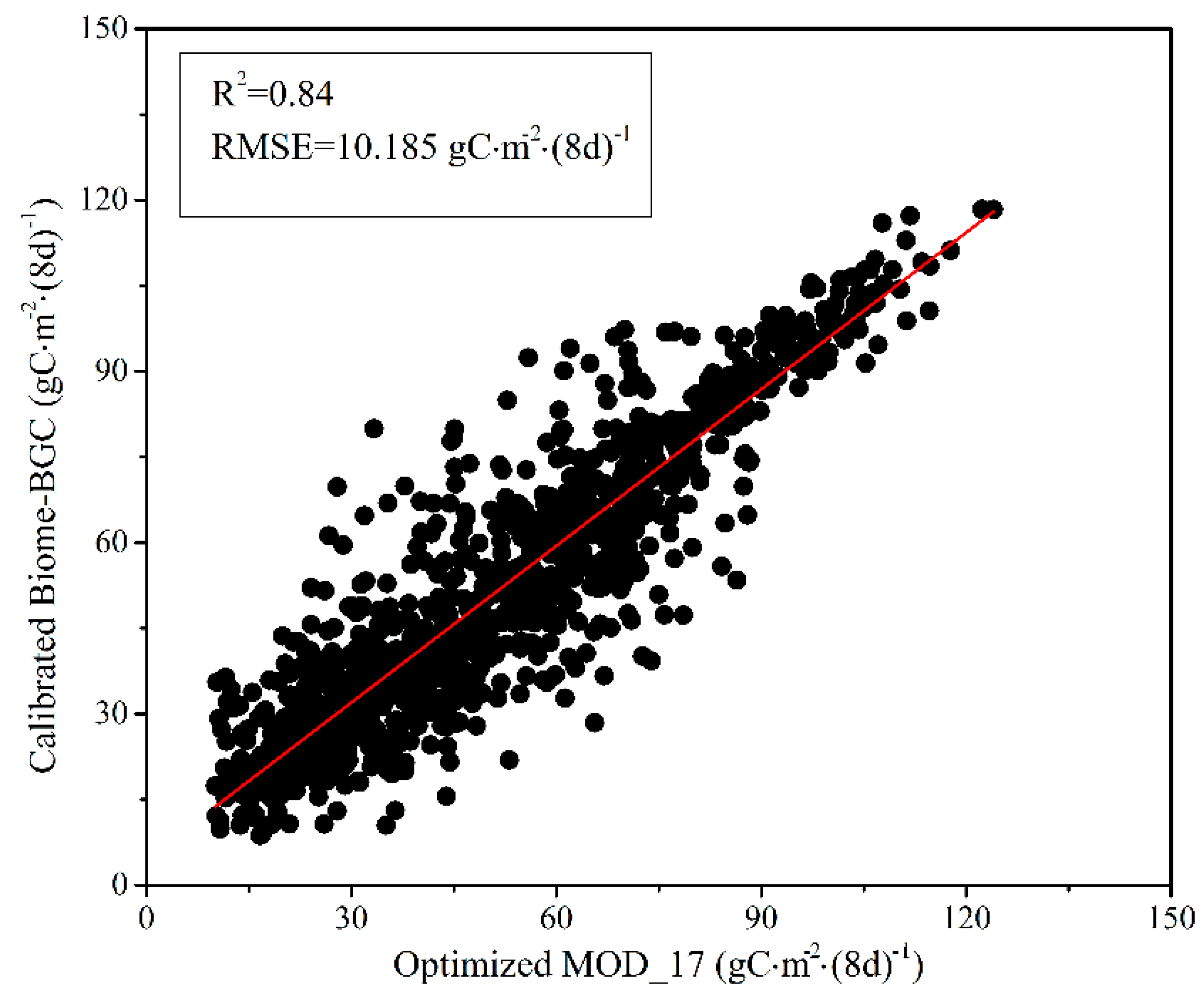
4.3. Calibration of Biome-BGC Model

A key determinant for the model to apply in a specific landscape or region is the parameterization, especially for the complicated process-based model. Here a preliminary calibration of the Biome-BGC model was conducted by incorporating the optimized MOD_17 model. Calibration was performed by adjusting the eight-day GPP outputs for the growing seasons from the Biome-BGC model in order to fit those obtained from the optimized MOD_17 model for the 10 selected forest plots. Sensitive (St > 0.1) parameters were calibrated accordingly once the best agreement was determined. During calibration, the sensitive parameters varied by 10% in both directions from the mean values reported by White et al. [10]. A scatter plot (Figure 4) indicates optimal agreement between growing season GPP values obtained from the optimized MOD_17 model and those from the calibrated Biome-BGC model (R2 = 0.84, RMSE = 10.185 gC·m−2·(8d)−1).

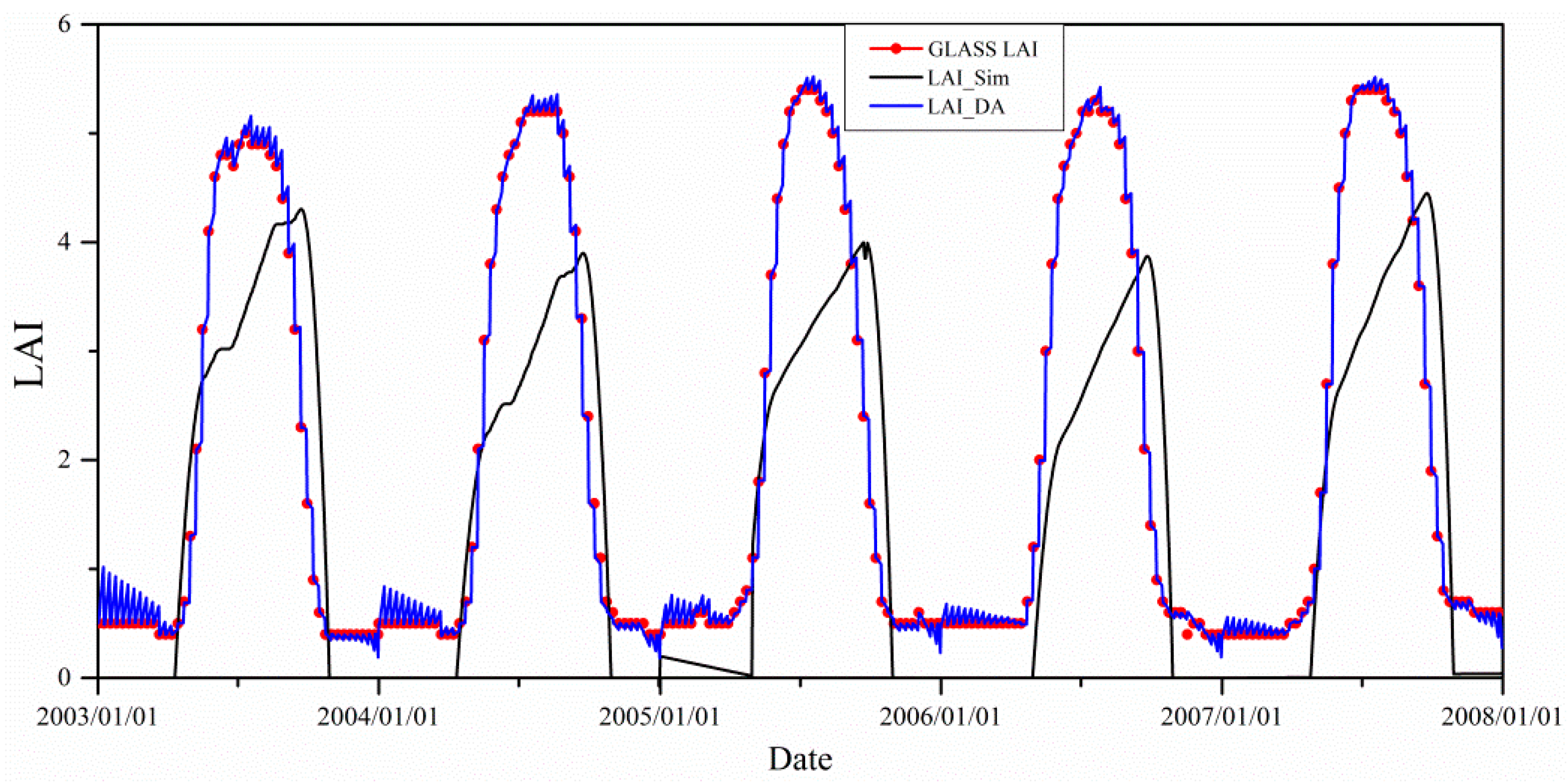
4.4. Carbon Fluxes from the Calibrated and Assimilated Model

Five years of GLASS LAI products were assimilated into the calibrated Biome-BGC model using the EnKF with an assimilation window of eight days. When the size of the ensemble was larger than 100, the R2 and RMSE between predicted GPP and EC measurements reached approximately stable values. The errors (from the model and GLASS LAI) were determined through LAI sites all over the world reported by Xiao et al. [47]. The error of GLASS LAI products ranged from −0.008 to 0.12. Then the variance (0.032) was calculated and used in the EnKF algorithm. The model error was estimated at the same time, and the value ranged from −0.32 to 0.44, with a variance of 0.616 in EnKF.
Figure 5 shows the comparison between GLASS LAI and simulated LAI, depicted as: LAI_sim (LAI obtained from the calibrated Biome-BGC without data assimilation) and LAI_DA (LAI simulated by the assimilated Biome-BGC model using the EnKF). It is noticeable that LAI_sim generally underestimated LAI compared with the observations, especially in growing seasons. LAI_sim increased rapidly at the beginning of the growing season and the values were higher than the remote sensing observations at the end of the growing season. The LAI_DA agreed well with the GLASS LAI, except for a few fluctuations in winter.
The measured GPP profile from 2003 to 2007 is shown in Figure 6a, together with those obtained from the default (GPP_Default), calibrated (GPP_Calibrated) and assimilated Biome-BGC model (GPP_DA). The original model was incapable of simulating GPP behavior, especially in summer and winter (Figure 6b, R2 = 0.72, RMSE = 2.419 gC·m−2·d−1). After calibration, the underestimation during summer had significantly diminished by adjusting the key parameters (FLNR, SLA, Gmax, etc.), with R2 = 0.87, and RMSE = 1.583 gC·m−2·d−1 (Figure 6c). However, some fluctuations still remained, especially in spring. Therefore the time series GLASS LAI was assimilated into Biome-BGC. The LAI was calculated from leaf carbon in Biome-BGC, and the assimilation directly affected the photosynthesis, thus affecting the performance of GPP. Figure 6d shows that GPPs from the assimilated Biome-BGC agreed well with the EC measurements.

5. Discussion

GPP estimates obtained from the optimized MOD_17 model performed well in this study, and thus provided the possibility of incorporating the remote sensing-based model with the process-based model (Biome-BGC) to acquire the carbon fluxes with temporal and spatial continuity. Furthermore, this strategy provided the option of circumventing the problem of scarce field data describing the various forest processes in specific biomes. Previous investigations have applied this method in a Mediterranean forest ecosystem [44,48,49], but the errors caused by the uncertainties in the remote sensing-based model would there be propagated to the next calibration and the predictions of carbon fluxes; the calibration of the parameters mainly focused on the parameters related to summer drought without considering exhaustive sensitivity analysis of other crucial parameters or a global calibration. Additionally, many studies concentrating on the calibration of Biome-BGC using field measurements (e.g., dendrochronological data, eddy covariance measurements) were carried out without considering temporal continuity or spatial heterogeneity based on reliable remote sensing data [50,51].
The results of sensitivity analysis showed that the total sensitivity indices of the crucial parameters were the main contributors to the annual mean GPP. This means that one parameter may enlarge the effects of other parameters [52]. The interaction effects of FLNR showed the highest influence on the annual mean GPP. FLNR controls the carboxylation capacity (Vcmax), which is the first step in the fixing of CO2 by the ribulose-1, 5-biphosphate protein [53]. Vcmax is a state variable in Biome-BGC with high spatial variability, so it is difficult to acquire [54]. The SLA also made contributions to the annual mean GPP by affecting the LAI. Gmax controlled the leaf conductance and was crucial for regulating water loss and carbon assimilation. The Wint coefficient determined the amount of precipitation intercepted by the canopy, which in turn controlled the amount of precipitation infiltrating [50]. With the interactions between the sensitive parameters being so extensive, the correlation between the input parameters should be further considered in a comprehensive calibration of the Biome-BGC. EnKF sequential data assimilation is an efficient way to improve the simulated carbon fluxes, capable of tracing the seasonal estimates of model outputs. As a key indicator of vegetation growth, the time series GLASS LAI was assimilated into the Biome-BGC model. These products of higher quality than the MODIS LAI were validated by Xiao et al. [47] at sites worldwide. The estimates of errors from GLASS LAI and model structure were important to the EnKF algorithm as the errors determined the extent to which the model predictions could be corrected. Considering the drawbacks of Biome-BGC in describing the water cycle [55], it is necessary to assimilate a soil moisture parameter into the model to improve the performance of evapotranspiration and soil moisture. The assimilation of long-term remote sensing observations (e.g., LAI, soil moisture) into process-based models could provide information on forest disturbance, an avenue that needs to be explored in further work.
The strategy explored in this study could be applied in long-term simulations of forest carbon fluxes over large regions and even facilitate analyzing the response of carbon fluxes to climatic variation. The reliability of the strategy has recently been proved in our study conducting long-term (between 2000 and 2012) validation of regional net primary productivity using dendrochronological data over the Qilian Mountains (R2 = 0.73, RMSE = 24.46 gC·m2·a−1) [56]. However, annual estimates of forest carbon fluxes still have limitations, some of which could be improved by better data or better understanding of carbon fluxes using optimized methods. Long-term carbon storage will be influenced by different kinds of forest disturbances (e.g., afforestation, deforestation, tree mortality, wildfire). Therefore, research on how carbon fluxes relate to forest disturbances, land management, and soil conditions should be considered in long-term simulations. The five-yearly national forest inventories conducted in China could provide additional information on natural and human disturbance.

6. Conclusions

The optimization of the MOD_17 model using refined input data improved the forest GPP behavior compared with applying the original MODIS model driven by default parameters. The optimized model was then incorporated in the Biome-BGC model exploiting the powers of both models for the simulation of forest carbon fluxes. The incorporation is also beneficial for the calibration of ecophysiological parameters and can make Biome-BGC more resistant to the impact of environment variability. The key ecophysiological parameters were determined with a sensitivity analysis on Biome-BGC using EFAST, a global analysis method that could provide the first order sensitivity index and the total order sensitivity index of the parameters to model predictions. The results demonstrated that FLNR, SLA, and FRC:LC were the parameters most sensitive for the model output.
A data assimilation method using EnKF has been designed to improve the simulation of carbon fluxes and reduce the errors based on time series remote sensing observations (GLASS LAI). This method takes errors in observations, input data and model structure into account to ensure that the output behavior is consistent with the observations. Eight-day GLASS LAI products were assimilated into the calibrated Biome-BGC model from 2003 to 2007 at a Changbai Mountains forest flux site to track the model over time. It was found that GPP behavior was smoothed by the EnKF, especially in spring, with the performance generally improving significantly (R2 = 0.92, RMSE = 1.261 gC·m−2·d−1).
With the model calibration and data assimilation, GPP behavior showed good agreement with EC measurements at the forest flux site, and it is possible to simulate other forest processes (e.g., evapotranspiration, respiration) based on this strategy as well, both on a local and a regional scale.

Acknowledgments

This work was supported by the National Basic Research Program of China (973 Program) under grant 2013CB733404. The eddy covariance measurements in this study were obtained from ChinaFlux. We would also like to thank Beijing Normal University for providing the GLASS products. The soil data set has been provided by Data Center for Resources and Environmental Sciences, Chinese Academy of Sciences (RESDC) (http://www.resdc.cn).

Author Contributions

Min Yan is the principal author of this manuscript, having written the majority of the manuscript and contributed at all phases of the investigation. Xin Tian contributed to the interpretation of methods and provided suggestions about the structure. Zengyuan Li and Erxue Chen contributed to the field logistic and design. Xufeng Wang, Zongtao Han, and Hong Sun contributed to the data processing.

Conflicts of Interest

The authors declare no conflict of interest.

References

  1. Quéré, C.L.; Moriarty, R.; Andrew, R.M.; Canadell, J.G.; Sitch, S.; Korsbakken, J.I.; Friedlingstein, P.; Peters, G.P.; Andres, R.J.; Boden, T.A. Global Carbon Budget 2015. Earth Syst. Sci. Data 2015. [Google Scholar] [CrossRef] [Green Version]
  2. Federici, S.; Tubiello, F.N.; Salvatore, M.; Jacobs, H.; Schmidhuber, J. New estimates of CO2 forest emissions and removals: 1990–2015. Forest Ecol. Manag. 2015, 352, 89–98. [Google Scholar] [CrossRef]
  3. FAO. Agriculture, Forestry and Other Land Use Emissions by Sources and Removals by Sinks: 1990–2011 Analysis. Available online: http://www.fao.org/docrep/019/i3671e/i3671e.pdf (accessed on 25 April 2014).
  4. Baldocchi, D.; Bowling, D. Modelling the discrimination of 13CO2 above and within a temperate broad-leaved forest canopy on hourly to seasonal time scales. Plant Cell Environ. 2003, 2, 231–244. [Google Scholar] [CrossRef]
  5. Baldocchi, D.; Falge, E.; Gu, L.H.; Olson, R.; Hollinger, D.; Running, S.W.; Anthoni, P.; Bernhofer, C. FLUXNET: A new tool to study the temporal and spatial variability of ecosystem-scale carbon dioxide, water vapor, and energy flux densities. B Am. Meteorol. Soc. 2011, 11, 2415–2434. [Google Scholar] [CrossRef]
  6. Wu, J.B.; Guan, D.X.; Sun, X.M.; Yu, G.R.; Zhao, X.S.; Han, S.J.; Jin, C.J. Eddy flux corrections for CO2 exchange in broad-leaved Korean pine mixed forest of Changbai Mountains. Sci. China Ser. D Earth Sci. 2005, 48, 106–115. [Google Scholar]
  7. Schmid, H.P.; Lloyd, C.R. Spatial representatives and the location bias of flux footprints over inhomogeneous areas. Agric. For. Meteorol. 1999, 93, 195–209. [Google Scholar] [CrossRef]
  8. Churkina, G.; Schimel, D.; Braswell, B.H.; Xiao, X. Spatial analysis of growing season length control over net ecosystem exchange. Glob. Chang. Biol. 2005, 11, 1777–1787. [Google Scholar] [CrossRef]
  9. Quaife, T.; Lewis, P.; Kauwe, M.D.; Williams, M.; Law, B.E.; Disney, M.; Bowyer, P. Assimilating canopy reflectance data into an ecosystem model with an Ensemble Kalman Filter. Remote Sens. Environ. 2008, 112, 1347–1364. [Google Scholar] [CrossRef]
  10. White, M.A.; Thornton, P.E.; Running, S.W.; Nemani, R.R. Parameterization and sensitivity analysis of the BIOME-BGC terrestrial ecosystem model: Net primary production controls. Earth Interact. 2000, 3, 1–85. [Google Scholar] [CrossRef]
  11. Verbeeck, H.; Samson, R.; Verdonck, F.; Lemeur, R. Parameter sensitivity and uncertainty of the forest carbon flux model FORUG: A Monte Carlo analysis. Tree Physiol. 2006, 26, 807–817. [Google Scholar] [CrossRef] [PubMed]
  12. Xiao, J.F.; Davis, K.J.; Urban, N.M.; Keller, K. Uncertainty in model parameters and regional carbon fluxes: A model-data fusion approach. Agric. For. Meteorol. 2014, 189–190, 175–186. [Google Scholar] [CrossRef]
  13. Moradkhani, H.; Hsu, K.L.; Gupta, H.; Sorooshian, S. Uncertainty assessment of hydrologic model states and parameters: Sequential data assimilation using the particle filter. Water Resour. Res. 2005, 41, W05012. [Google Scholar] [CrossRef]
  14. Evensen, G. Sequential data assimilation with a nonlinear quasigeostrophic model using Monte Carlo methods to forecast error statistics. J. Geophys. Res. 1994, 99, 10143–10162. [Google Scholar] [CrossRef]
  15. Evensen, G. The Ensemble Kalman Filter: Theoretical formulation and practical implementation. Ocean Dyn. 2003, 53, 343–367. [Google Scholar] [CrossRef]
  16. Williams, M.; Schwarz, P.A.; Law, B.E.; Irvine, J.; Kurpius, M.R. An improved analysis of forest carbon dynamics using data assimilation. Glob. Chang. Biol. 2005, 11, 89–105. [Google Scholar] [CrossRef]
  17. Zhao, Y.X.; Chen, S.N.; Shen, S.H. Assimilating remote sensing information with crop model usingEnsemble Kalman Filter for improving LAI monitoring and yield estimation. Ecol. Model. 2013, 270, 30–42. [Google Scholar] [CrossRef]
  18. Wang, X.X.; Ma, M.G.; Han, X.J.; Song, Y. Assimilation of soil moisture in LPJ-DGVM. Proc. SPIE 2009, 7472. [Google Scholar] [CrossRef]
  19. Mo, X.G.; Chen, J.M.; Ju, W.M.; Andrew Black, T. Optimization of ecosystem model parameters through assimilating eddy covariance flux data with an ensemble Kalman filter. Ecol. Model. 2008, 217, 157–173. [Google Scholar] [CrossRef]
  20. Migliavacca, M.; Meroni, M.; Busetto, L.; Colombo, R.; Zenone, T.; Matteucci, G.; Iovanni, M.G.; Seufert, G. Modeling gross primary production of agro-forestry ecosystems by assimilation of satellite-derived information in a process-based model. Sensors 2009, 9, 922–942. [Google Scholar] [CrossRef] [PubMed] [Green Version]
  21. Demarty, J.; Chevallier, F.; Friend, A.D.; Viovy, N.; Piao, S.L.; Ciais, P. Assimilation of global MODIS leaf area index retrievals within a terrestrial biosphere model. Geophys. Res. Lett. 2007, 34, L15402. [Google Scholar] [CrossRef]
  22. Wang, Q.F.; Niu, D.; Yu, G.R.; Ren, C.Y.; Wen, X.F.; Chen, J.M.; Ju, W.M. Simulating the exchange of carbon dioxide, water vapor and heat over Changbai Mountains temperate broad-leaved Korean pine mixed forest ecosystem. Sci. China Ser. D Earth Sci. 2005, 48, 148–159. [Google Scholar]
  23. Running, S.W.; Nemani, R.R.; Hungerford, R.D. Extrapolation of synoptic meteorological data in mountainous terrain and its use for simulating forest evaporation and photosynthesis. Can. J. For. Res. 1987, 17, 472–483. [Google Scholar] [CrossRef]
  24. Thornton, P.E.; Running, S.W. An improved algorithm for estimating incident daily solar radiation from measurements of temperature, humidity, and precipitation. Agric. For. Meteorol. 1999, 93, 211–228. [Google Scholar] [CrossRef]
  25. Thornton, P.E.; Running, S.W.; White, M.A. Generating surfaces of daily meteorological variables over large regions of complex terrain. J. Hydrol. 1997, 190, 214–251. [Google Scholar] [CrossRef]
  26. Xiao, Z.Q.; Liang, S.L.; Sun, R.; Wang, J.D.; Jiang, B. Estimating the fraction of absorbed photosynthetically active radiation from the MODIS data based GLASS leaf area index product. Remote Sens. Environ. 2015, 171, 105–117. [Google Scholar] [CrossRef]
  27. Monteith, J. Solar radiation and productivity in tropical ecosystems. J. Appl. Ecol. 1972, 747–766. [Google Scholar] [CrossRef]
  28. Jahan, N.; Gan, T.Y. Modeling gross primary production of deciduous forest using remotely sensed radiation and ecosystem variables. J. Geophys. Res.: Biogeosci. 2009, 114. [Google Scholar] [CrossRef]
  29. Hansen, M.C.; DeFries, R.S.; Townshend, J.R.G.; Sohlberg, R. Global land cover classification at 1 km spatial resolution using a classification tree approach. Int. J. Remote Sens. 2000, 21, 1331–1364. [Google Scholar] [CrossRef]
  30. Running, S.W.; Nemani, R.R.; Heinsch, F.A.; Zhao, M.S.; Reeves, M.; Hashimoto, H. A continuous satellite-derived measure of global terrestrial primary production. Bioscience 2004, 54, 547–560. [Google Scholar] [CrossRef]
  31. Coops, N.C.; Black, T.A.; Jassal, R.P.S.; Trofymow, J.T.; Morgenstern, K. Comparison of MODIS, eddy covariance determined and physiologically modelled gross primary production (GPP) in a Douglas-fir forest stand. Remote Sens. Environ. 2007, 107, 385–401. [Google Scholar] [CrossRef]
  32. Nightingale, J.M.; Coops, N.C.; Waring, R.H.; Hargrove, W.W. Comparison of MODIS gross primary production estimates for forests across the USA with those generated by a simple process model, 3-PGS. Remote Sens. Environ. 2007, 109, 500–509. [Google Scholar] [CrossRef]
  33. Turner, D.P.; Ritts, W.D.; Zhao, M.S.; Kurc, S.; Dunn, A.L.; Wofsy, S.C.; Small, E.E.; Running, S.W. Assessing interannual variation in MODIS-based estimates of gross primary production. IEEE Trans. Geosci. Remote Sens. 2006, 44, 1899–1907. [Google Scholar] [CrossRef]
  34. Reeves, M.C.; Zhao, M.; Running, S.W. Usefulness and limits of MODIS GPP for estimating wheat yield. Int. J. Remote Sens. 2005, 26, 1403–1421. [Google Scholar] [CrossRef]
  35. Gebremichael, M.; Barros, A.P. Evaluation of MODIS gross primary productivity (GPP) in tropical monsoon regions. Remote Sens. Environ. 2006, 100, 150–166. [Google Scholar] [CrossRef]
  36. Zhang, Y.Q.; Yu, Q.; Jiang, J.E.; Tang, Y.H. Calibration of Terra/MODIS gross primary production over an irrigated cropland on the North China Plain and an alpine meadow on the Tibetan Plateau. Glob. Chang. Biol. 2008, 14, 757–767. [Google Scholar] [CrossRef]
  37. Propastin, P.; Ibrom, A.; Knohl, A.; Erasmi, S. Effects of canopy photosynthesis saturation on the estimation of gross primary productivity from MODIS data in a tropical forest. Remote Sens. Environ. 2012, 121, 252–260. [Google Scholar] [CrossRef]
  38. Jin, C.; Xiao, X.M.; Merbold, L.; Arneth, A.; Veenendaal, E.; Kutsch, W.L. Phenology and gross primary production of two dominant savanna woodland ecosystems in Southern Africa. Remote Sens. Environ. 2013, 135, 189–201. [Google Scholar] [CrossRef]
  39. Liu, Z.J.; Shao, Q.Q.; Liu, J.Y. The performances of MODIS-GPP and -ET products in China and their sensitivity to input data (FPAR/LAI). Remote Sens. 2015, 7, 135–152. [Google Scholar] [CrossRef]
  40. Chen, J.; Zhang, H.F.; Liu, Z.R.; Che, M.L.; Chen, B.Z. Evaluating parameter adjustment in the MODIS gross primary production algorithm based on eddy covariance tower measurements. Remote Sens. 2014, 6, 3321–3348. [Google Scholar] [CrossRef]
  41. Heinsch, F.A.; Reeves, M.; Votava, P.; Ang, S.; Ilesi, C.; Hao, M.; Lassy, J.; Jolly, W.M.; Loehman, R.; Bowker, C.F. GPP and NPP (MOD17A2/A3) Products NASA MODIS Land Algorithm. In MOD17 User’s Guide; NASA: Missoula, MT, USA, 2003; pp. 1–57. [Google Scholar]
  42. Farquhar, G.D.; Caemmerer, S.; Berry, J.A. A biochemical model of photosynthetic CO2 assimilation in leaves of species. Planta 1980, 149, 78–90. [Google Scholar] [CrossRef] [PubMed]
  43. Zhang, T.L.; Sun, R.; Peng, C.H.; Zhou, G.Y.; Wang, C.L.; Zhu, Q.A.; Yang, Y.Z. Integrating a model with remote sensing observations by a data assimilation approach to improve the model simulation accuracy of carbon flux and evapotranspiration at two flux sites. Sci. China Earth Sci. 2016, 59, 337–348. [Google Scholar] [CrossRef]
  44. Chiesi, M.; Chirici, G.; Barbati, A.; Salvati, R.; Maselli, F. Use of BIOME-BGC to simulate Mediterranean forest carbon stocks. iForest 2010, 4, 121–127. [Google Scholar] [CrossRef]
  45. Saltelli, A. Sensitivity analysis for importance assessment. Risk Anal. 2002, 22, 579–590. [Google Scholar] [CrossRef] [PubMed]
  46. Wang, X.F.; Ma, M.G.; Li, X.; Song, Y.; Tan, J.L.; Huang, G.H.; Zhang, Z.H.; Zhao, T.B.; Feng, J.M.; Ma, Z.G. Validation of MODIS-GPP product at 10 flux sites in northern China. Int. J. Remote Sens. 2013, 34, 587–599. [Google Scholar] [CrossRef]
  47. Xiao, Z.Q.; Liang, S.L.; Wang, J.D.; Chen, P.; Yin, X.J.; Zhang, L.Q.; Song, J.L. Use of general regression neural networks for generating the GLASS leaf area index product from time-series MODIS surface reflectance. IEEE Trans. Geosci. Remote Sens. 2014, 52, 209–223. [Google Scholar] [CrossRef]
  48. Chiesi, M.; Maselli, F.; Moriondo, M.; Fibbi, L.; Bindi, M.; Running, S.W. Application of BIOME-BGC to simulate Mediterranean forest processes. Ecol. Model. 2007, 206, 179–190. [Google Scholar] [CrossRef]
  49. Chiesi, M.; Fibbi, L.; Genesio, L.; Gioli, B.; Magno, R.; Maselli, F.; Moriondo, M.; Vaccari, F.P. Integration of ground and satellite data to model Mediterranean forest processes. Int. J. Appl. Earth Obs. 2011, 13, 504–515. [Google Scholar] [CrossRef]
  50. Chiesi, M.; Maselli, F.; Bindi, M.; Fibbi, L.; Cherubini, P.; Arlotta, E.; Tirone, G.; Matteucci, G.; Seufert, G. Modelling carbon budget of Mediterranean forests using ground and remote sensing measurements. Agric. For. Meteorol. 2005, 135, 22–34. [Google Scholar] [CrossRef]
  51. Hidy, D.; Barcza, Z.; Haszpra, L.; Churkina, G.; Pintér, K.; Nagy, Z. Development of the Biome-BGC model for simulation of managed herbaceous ecosystems. Ecol. Model. 2012, 226, 99–119. [Google Scholar] [CrossRef]
  52. Miao, Z.W.; Lathrop, R.G., Jr.; Xu, M.; La Puma, I.P.; Clark, K.L.; Hom, J.; Skowronski, N.; Van Tuyl, S. Simulation and sensitivity analysis of carbon storage and fluxes in the New Jersey Pinelands. Environ. Model. Soft. 2011, 26, 1112–1122. [Google Scholar] [CrossRef]
  53. Raj, R.; Hamm, N.A.S.; van der Tol, C.; Stein, A. Variance-based sensitivity analysis of BIOME-BGC for gross and net primary production. Ecol. Model. 2014, 292, 26–36. [Google Scholar] [CrossRef]
  54. Houborg, R.; Cescatti, A.; Migliavacca, M. Constraining model simulations of GPP using satellite retrieved leaf chlorophyll. In Proceedings of the IEEE International Geoscienceand Remote Sensing Symposium (IGARSS), Munich, Germany, 22–27 July 2012; pp. 6455–6458.
  55. Kimball, J.S.; White, M.A.; Running, S.W. Biome-BGC simulations of stand hydrologic processes for BOREAS. J. Geophys. Res. 1997, 102, 29043–29051. [Google Scholar] [CrossRef]
  56. Yan, M.; Tian, X.; Li, Z.Y.; Chen, E.X.; Li, C.M.; Fan, W.W. A long-term simulation of forest carbon fluxes over the Qilian Mountains. Int. J. Appl. Earth Obs. 2016. under review. [Google Scholar]
Figure 1. The overall flowchart of this study.
Remotesensing 08 00567 g001
Figure 2. Seasonal performances (a) and comparisons (b) of eight-day GPPs obtained from the original products (GPP_Default), three simulations (GPP_MOD1, GPP_MOD2, and GPP_MOD3), and EC measurements (GPP_EC) at Changbai Mountains forest flux site between 2003 and 2007.
Remotesensing 08 00567 g002
Figure 3. The first order and total order sensitivity indexes for annual mean GPP.
Remotesensing 08 00567 g003
Figure 4. A comparison of eight-day GPP values for the growing season obtained using the optimized MOD_17 model and those derived from the calibrated Biome-BGC model.
Remotesensing 08 00567 g004
Figure 5. Comparison of simulated LAI and GLASS LAI.
Remotesensing 08 00567 g005
Figure 6. Results of default, calibrated, and assimilated GPP: (a) Performances of GPPs from the EC measurement, default, calibrated and assimilated Biome-BGC; (b) comparison and validation of GPP values from the EC measurement and default Biome-BGC; (c) comparison and validation of GPP values from the EC measurement and calibrated Biome-BGC; (d) comparison and validation of GPP values from the EC measurement and assimilated Biome-BGC.
Remotesensing 08 00567 g006aRemotesensing 08 00567 g006b
Table 1. Distribution of Biome-BGC crucial ecophysiological parameters [10].
ParameterDescriptionUnitDistribution a
FRC:LCNew fine C: new leaf CkgC (kgC)−1U(0.53, 6.5)
SC:LCNew stem C: new leaf CkgC (kgC)−1U(0.62, 4.9)
LWC:TWCNew live wood C: new total wood CkgC (kgC)−1U(0.028, 0.189)
CRC:SCNew croot C: new stem CkgC (kgC)−1U(0.12, 0.7)
CGPCurrent growth proportionProp.U(0.25, 0.75)
C:NleafC:N of leaveskgC (kgN)−1N(34.5, 5.4)
C:NlitC:N of leaf litterkgC (kgN)−1N(55, 16)
C:NfrC:N of fine rootkgC (kgN)−1N(48, 15)
C:NdwC:N of dead woodkgC (kgN)−1U(300, 800)
LcelLeaf litter cellulose proportion%N(0.2, 0.01)
LligLeaf litter lignin proportion%N(0.18, 0.0008)
FRcelFine root cellulose proportion%U(0.2, 0.6)
FRligFine root lignin proportion%U(0.1, 0.5)
DWligDead wood lignin proportion%N(0.23, 0.0049)
WintCanopy water interception coefficientLAI−1day−1N(0.045, 0.012)
KCanopy light extinction coefficientUnitlessN(0.4, 0.007)
LAIall:projAll-sided to projected leaf area ratioLAI LAI−1U(2.3, 3.14)
SLACanopy average specific leaf aream2 (kgC)−1N(25, 10)
FLNRFraction of leaf N in RubiscoUnitlessU(0.01, 1)
GmaxMaximum stomatal conductancems−1N(0.005, 0.0007)
GblBoundary layer conductancems−1N(0.03, 0.12)
LWPiLeaf water potential: start of conductance reductionMpaU(−1.11, −0.21)
LWPfLeaf water potential: complete conductance reductionMpaU(−5, −1)
VPDiVapor pressure deficit: start of conductance reductionPaU(500, 1000)
VPDfVapor pressure deficit: complete conductance reductionPaU(2000, 6000)
a U(min, max): uniform distribution, N (mean, standard deviation): normal distribution.

