A Conceptually Simple Modeling Approach for Jason-1 Sea State Bias Correction Based on 3 Parameters Exclusively Derived from Altimetric Information

Abstract

A conceptually simple formulation is proposed for a new empirical sea state bias (SSB) model using information retrieved entirely from altimetric data. Nonparametric regression techniques are used, based on penalized smoothing splines adjusted to each predictor and then combined by a Generalized Additive Model. In addition to the significant wave height (SWH) and wind speed (U10), a mediator parameter designed by the mean wave period derived from radar altimetry, has proven to improve the model performance in explaining some of the SSB variability, especially in swell ocean regions with medium-high SWH and low U10. A collinear analysis of scaled sea level anomalies (SLA) variance differences shows conformity between the proposed model and the established SSB models. The new formulation aims to be a fast, reliable and flexible SSB model, in line with the well-settled SSB corrections, depending exclusively on altimetric information. The suggested method is computationally efficient and capable of generating a stable model with a small training dataset, a useful feature for forthcoming missions.

1. Introduction

Sea state bias (SSB) is an altimeter ranging error caused by the influence of sea-state effects in the radar altimeter measurements, since the surface scattering elements do not contribute equally to the radar return. Usually, the SSB is characterized by the sum of three different contributions. An electromagnetic bias (EM) evidenced by the signal-surface interactions, where ocean wave troughs are better radar reflectors than wave crests, thus overestimating the measured satellite-to-surface range. The EM bias perturbs all microwave frequencies with wavelengths of a few centimeters, affecting not only the Ka-, C-, and Ku-bands regularly used for satellite altimetry [1,2], but also the L-band frequency usually adopted for Global Navigation Satellite Systems Reflectometry (GNSS-R) altimetry [3]. In addition to EM bias, the SSB is also characterized by a skewness bias linked to the effect of a non-Gaussian surface height distribution, inducing an error due to the difference between the determined median sea surface and the true mean sea surface (MSS), and finally, a tracker bias which can occur due to both instrumental and retracking effects. With an order of magnitude ranging between 3%–4% of the significant wave height (SWH), this centimeter-scale measurement bias remains as one of the largest sources of uncertainty linked with the altimetric signal.

Historically, the parametric SSB models started to be developed as a simple linear empirical model using a first-order predictor expressed in the normalized form as α = SSB/SWH due to the strong dependency of SSB with SWH [4]. Later on, SSB estimates were obtained using fitted empirical models derived from two predictors retrieved from the analysis of altimeter data, the altimeter-derived SWH and wind speed (U10), with the latter based on radar backscatter cross-section measurements (σ⁰). Since then, different statistical approaches have been considered to better characterize the SSB, parametric formulations of both SWH and U10 in linear, polynomial or quadratic forms, estimating a number of coefficients [5], and nonparametric techniques using different statistical approaches as the kernel smoothing method [6], local linear kernel smoothing [7] or smoothing splines [8]. Before fitting the models, SSB estimates can be retrieved by sea surface height (SSH) differences at crossover points, along collinear tracks or directly estimated from the residuals between SSH and an MSS over the SWH and U10 domain [9]. More recently, [10] suggested that these methods, solely based on wave and wind information from the altimeter may be improved if additional surface gravity wave field measurements become available from numerical ocean wave model data, leading to an enhanced 3-dimensional (3D) SSB model derived from SWH, U10 and a third predictor characterized by the mean wave period (Tm), retrieved from WAVEWATCH III (WW3) [11]. This improved SSB model achieves positive results in reducing SSH variance both at global and regional scales, but the required external information from WW3 adds a new source of uncertainty which may not be directly related to the altimetric signal.

In another field of study, several models have been proposed [12,13,14,15,16,17] to retrieve the wave period information (Tm, Tz) exclusively from the radar altimeter signal, combining both SWH and σ⁰. In the scope of this paper, the algorithms proposed by [14,15] were selected for evaluation, due to their simplicity, ease of implementation and good agreement when compared with buoy measurements. This paper proposes a simple formulation for a new SSB empirical model using three predictors (SWH, U10, Tz) solely derived from altimetric information, fitted with smoothing splines methods embedded in a general framework provided by Generalized Additive Models (GAMs).

The paper is organized as follows. Section 2 describes all the methodology used for model design. The approach used to estimate reliable SSB predictions, is explained in Section 2.1. The considered mean wave period algorithms for this study are exposed in Section 2.2 and the chosen nonparametric statistical approach is presented in Section 2.3. All the obtained results are shown in Section 3. Section 4 and Section 5 provide discussion and conclusions.

2. Data and Methods

All the satellite altimeter and WW3 data were retrieved from the Radar Altimeter Database System (RADS), a validated and cross-calibrated source of Geophysical Data Records (GDRs) for all altimetric missions, incorporating the most up-to-date altimeter data, the latest instrument and geophysical corrections from several external datasets and models [18,19]. RADS delivers a consistent altimeter database at 1-Hz, flexible enough to construct the sea level anomaly (SLA) either from a predefined or user-defined criteria.

Table 1. Description of the various Radar Altimeter Database System (RADS) parameters and limits used. For this sea state bias (SSB) study, the limits of significant wave height (SWH), wind speed (U10) and σ⁰ were chosen in order to use all the available information. Parameters min, max and RADS reference code are presented.

Name (Units)	Code	Min	Max
sea level anomaly (m)	0	−5	5
latitude (degrees)	201	−60	60
Ku-band significant wave height (m)	1701	0	10
altimeter wind speed (m/s)	1901	0	30
Ku-band backscatter coefficient (dB)	1801	0	16
std dev of Ku-band range (m)	2002	0	0.4
number of valid Ku-band measurements	2101	16	21
surface type	2504	0 = open ocean
corruption of altimeter measurement	flag7	0 = ok

describes the most relevant parameters and chosen criteria used for querying and retrieving the database information. This work concerns the entire phase A of Jason-1 mission, from cycle 001 to 260. The main reasons for this choice were the fact that we are dealing with one of the longest altimetric missions with a time span from 15 January 2002 to 26 January 2009 and because the two most used and widely accepted SSB models, the CLS nonparametric sea state bias (SSB CLS) from [7] and the nonparametric sea state bias combined with WW3 (SSB Tran) from [11] are available for this mission, thus allowing an in-depth comparative analysis with the proposed model from this study.

2.1. Direct Estimation of Sea State Impacts

An empirical determination of the SSB correction from the altimeter measurements is frequently made by extracting the related signal from sea surface height measurements. Before any SSB determination, a careful analysis of the SSH observations is necessary to detect possible instrumental or geophysical errors in order to avoid non-SSB signals which may corrupt the estimates to be modeled afterwards. The SSH measured at one particular location and uncorrected for SSB, contains the geoid signal (h_g), the ocean dynamic topography (η), the SSB effect and all other instrumental and geophysical errors represented by (ω):

$$SSH=h_g+\eta +SSB+\omega$$

(1)

Usually, the SSB is estimated by differencing the repeated measurements either along collinear tracks [20] or at orbit crossover points [5], but [9] proposed a simpler direct technique where sea height deviations from the marine geoid are binned against altimeter U10 and SWH, becoming an easier method to implement, directly solving for SSB by imposing a constant a priori mean sea level at each altimeter observation location thus eliminating the geoid. The following equation represents this relation:

$$SSB{\left(U10,\mathrm{SWH}\right)}_{bin}={〈\left(SSH-MSS\right)〉}_{bin}$$

(2)

where the left side of Equation (2) denotes the SSB estimation in U10 and SWH domains, function of the difference between SSH and MSS, bin-averaged for the same domain. Besides the ease of implementation, another big advantage of the direct method is the high resolution of the final estimation, allowing to the determine a more detailed model when compared with other methods. Some disadvantages of this technique should be considered, the presence of some noisy estimates near the domain limits requires a proper treatment, and the impossibility to compute SSB estimations outside the domain range confined by the limits of SWH and U10 [21]. In this work, the direct estimation of sea state impacts was implemented in order to give a reliable SSB prediction, used as an input for the final response which will be modeled.

2.2. Mean Zero Up-Crossing Period (T_m, T_z)

The wave period parameter is characterized by the interval between successive waves, obtained by averaging all wave periods measured in a time interval divided by the number of waves in this interval. A special case is the mean zero-crossing period $\overline{T_0}$ described by:

$$\overline{T_0}=T_{m_{02}}=T_z=\sqrt{m_0/m_2}$$

(3)

where $m_0$ and $m_2$ are the zeroth- and second-order moments of the variance density spectrum $E\left(f\right)$. In the scope of this work, $T_{m_{02}}=T_z$ was the chosen mean wave period parameter, due to its reliability and for a better comparison with the proposed mentioned wave period algorithms by [14] (hereafter G03) and [15] (hereafter Q04). G03 suggested a simple empirical model for wave period retrieval, using the Ku-band radar altimeter backscatter and significant wave height, formulated with an heuristic model based on collocated buoy observations and TOPEX altimeter data $T\sim {\left({\sigma }_L^{0}SW{H}^2\right)}^{0.25}$. The model was built by performing a linear regression in the log domain of wave period from T against with the altimeter ${\sigma }^0$ expressed in its linear (non-dB) form:

$$lo{g}_{10}\left(T_z\right)=0.361+0.967\ast lo{g}_{10}{\left({\sigma }_L^0{\mathrm{SWH}}^2\right)}^{0.25}$$

(4)

A regional assessment of the model was also performed by the authors, concluding that G03 is better suited to wind-dominated seas than to regions with swell. Additionally to this, [22] compared the G03 model with National Data Buoy Center (NDBC) buoys and the European Centre for Medium-Range Weather Forecasts (ECMWF) ERA-40 dataset, and suggested that altimeter-derived mean wave period is reliable even in swell conditions for moderate to high winds (above 4 m/s), in contrast to previous studies which limited its validity just to wind-dominated seas.

Based on the fact that ${\sigma }^0$ is related with the ocean surface wave mean square slope statistics, Q04 proposed two algorithms to estimate an altimeter-derived mean wave period using methods based on neural networks. A first method based solely on the altimeter Ku-band measurements, and an alternative method $T_{nn}^2$, the one that has been used in this work, which gathers information from both C and Ku band radar cross sections together with wind speed (U10) for a better constraint of the wind sea contribution. $T_{nn}^2$ operates with the dual-frequency capability of altimeters, thus allowing a better retrieval of the local environmental conditions and showing a good agreement with the mean wave period observations from NDBC buoys.

$$\begin{array}{c}\hfill T_{nn}^2=e^{\left(5.7474-1.4688\ast a+1.7943\ast b\right)},\text{with}\end{array}$$

(5)

$$\begin{array}{c}\hfill a=\frac{{\sigma }_{Ku}^{0.3082}}{{\sigma }_C^{0.2352}\ast {\mathrm{SWH}}^{0.0981}}\ast e^{1.5068\ast b},\text{and}b=\frac{2}{1+e^{\left(-1.8612-0.08\ast U_{10}\right)}}-1\end{array}$$

There is some discussion about the ${\sigma }^0$ upper limit that should be used, Q04 mention an upper threshold of 16 dB for Ku-band and 20 dB for C-band, considering that the measurements beyond these thresholds correspond to surface slicks for which there are no surface waves. On the other hand, [16] applied a threshold of 13 dB stating that above this value, ${\sigma }^0$ is no longer related to the wave period. For this work, a threshold of 16 dB for Ku-band ${\sigma }^0$ was applied, leaving the C-band free and the resulting mean wave period $T_z$ with a valid range between 1 s and 16 s, since outside this range there might be some inefficiency of the applied models.

2.3. Smoothing Splines with GAMs

The chosen approach for SSB modeling was based on smoothing spline methods embedded in a general framework provided by Generalized Additive Models (GAMs) [23,24]. The first thing that must be given attention to, is how to find a smooth curve that fits the observed data well, minimizing the residual sum of squares $RSS={\sum }_{i=1}^n{\left(y_i-g\left(x_i\right)\right)}^2$. Such a function has to be chosen carefully, otherwise it will be too flexible, overfitting the data. To accomplish this task, it is necessary to add a penalty term, penalizing steep slopes and variability of f:

$${\displaystyle \sum _{i=1}^n}{\left(y_i-f\left(x_i\right)\right)}^2+\lambda \int f^{″}{\left(t\right)}^{2}dt$$

(6)

the fitting procedure takes the new form of a loss+penalty function where λ is a nonnegative tuning parameter for roughness control and can be chosen manually, based on data variability analysis or by cross-validation techniques. The smoothing spline function $f\left(x\right)$ that minimizes Equation (6) is a piecewise cubic polynomial with a number of knots, smoothed by a continuous first and second derivatives. The SSB model was designed using a generalized additive model (GAM) thus extending the range of a multiple linear regression model and allowing nonlinear relationships between each predictor and the response:

$$Y_i={\beta }_0+f_1\left(x_{i1}\right)+f_2\left(x_{i2}\right)+\dots +f_p\left(x_{ip}\right)+{ϵ}_i$$

(7)

where a separate cubic regression spline $f_j$ with λ=6 was applied to each predictor $x_{ij}$ and added together in the final framework. The additive properties of the model allows an individual contribution analysis of each $x_{ij}$ on $Y_i$ while holding all the other variables fixed, providing this way a useful compromise between linear and fully nonparametric models. For this work, the goal was to design a SSB model using three predictors $\left(X_{i1},X_{i2},X_{i3}\right)=\left(SW{H}_i,U{10}_i,T_{z}G03\right)$, evaluating the impact of the third predictor in the final response, the goodness of fit, simplicity and smoothness, without data overfitting.

3. Results

The flowchart presented in Figure 1 attempts to clarify the main steps involved in the proposed SSB modeling and how they relate. After retrieving the satellite altimeter information from RADS, a careful selection criteria had to be applied, conditioning some parameters limits. The entire range of SWH and U10 up to the limits of 10 m and 30 m/s respectively, were considered. A bin-averaged procedure for the SWH-U10 domain has been applied, producing a preliminary training dataset which had to be supervised by subsetting and weighting strategies before feeding the model. A screening method for outliers detection has been implemented before the model testing phase.

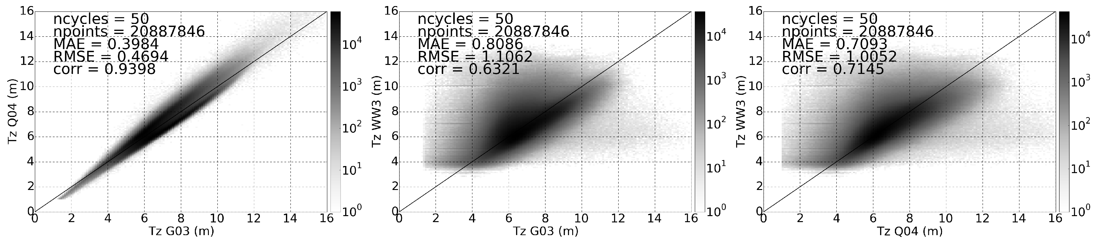
3.1. Mean Wave Period Assessment

Aiming at selecting an appropriate algorithm to determine the mean wave period from altimetric data, a thorough assessment was performed for the first 50 cycles of Jason-1, comparing G03, Q04 and the mean wave period $T_z=\sqrt{m_0/m_2}$, where $m_0$ and $m_2$ are the wave spectral moments of the wave model WW3 obtained from RADS. Three histograms are presented in Figure 2 showing that about 20 million measurements were considered valid.

As expected, the algorithms from G03 and Q04 have large correlations, higher than 0.9, and relatively low mean absolute and root mean square differences, pointing up that both models are coherent with each other for the considered data span. The right plot shows how G03 relates with the mean wave period derived from WW3. Despite the slightly worse results, with higher mean absolute and root mean square differences, the correlation between both datasets remains above 0.6. Similar results were obtained for Q04 (middle plot) revealing an identical behavior with G03 when compared with Tz from WW3. To overcome the systematic underestimation of the swell in WW3 pointed by Q04 and the suggested evidence that G03 is better suited for wind-dominated seas than to swell regions, [22] defined a swell ratio (SR) characterized by the ratio between the swell wave height directly retrieved from the numerical wave model, and the SWH obtained from the model zeroth-order moment of the variance density spectrum with $4\sqrt{m_0}$. Taking advantage of the fact that RADS provides the swell wave height of WW3, it was possible to define a SR < 0.9, applied to the initial dataset, thus filtering out measurements from swell-dominated sea states. Figure 3 shows a new set of two-dimensional histograms and associated statistics when SR is activated.

As shown in Figure 3, when the SR limit is activated, the number of measurements decreases by about 30%. The correlation between G03 and Q04 algorithms is still extremely high, but unlike the previous scenario, here the correlation between G03 algorithm and WW3 model increases considerably to values higher than 0.8, suggesting that G03 is better related with the part of the wave spectrum that is under direct influence of the wind, particularly wind seas directly generated and affected by local winds. Again, a similar behavior is obtained for Q04 when compared with WW3, highlighting the similarities between the two considered algorithms. Despite the better results, SR was not considered for the development design of SSB model in this study, since the swell wave height is a parameter exclusively retrieved from numerical wave models and not from altimeter data. To complement this assessment, a global spatial analysis covering the first 50 cycles of Jason-1 was performed, correlating G03 and Q04 with the mean wave period derived from WW3, shown in Figure 4. It is clear to observe a latitude dependency with an increase of correlation for higher latitudes, but overall, there is a good statistical relationship between both algorithms when related with WW3.

After a careful analysis of the two mean wave period algorithms and how they relate with the same parameter derived from the numerical wave model, it is safe to assume that both G03 and Q04 algorithms produce similar estimates when compared against WW3 model retrieved from RADS. Due to a simpler approach and ease of implementation, G03 was the chosen algorithm to be the third predictor of SSB modeling, mediating the relationship between SWH and U10 retrieved from the altimeter.

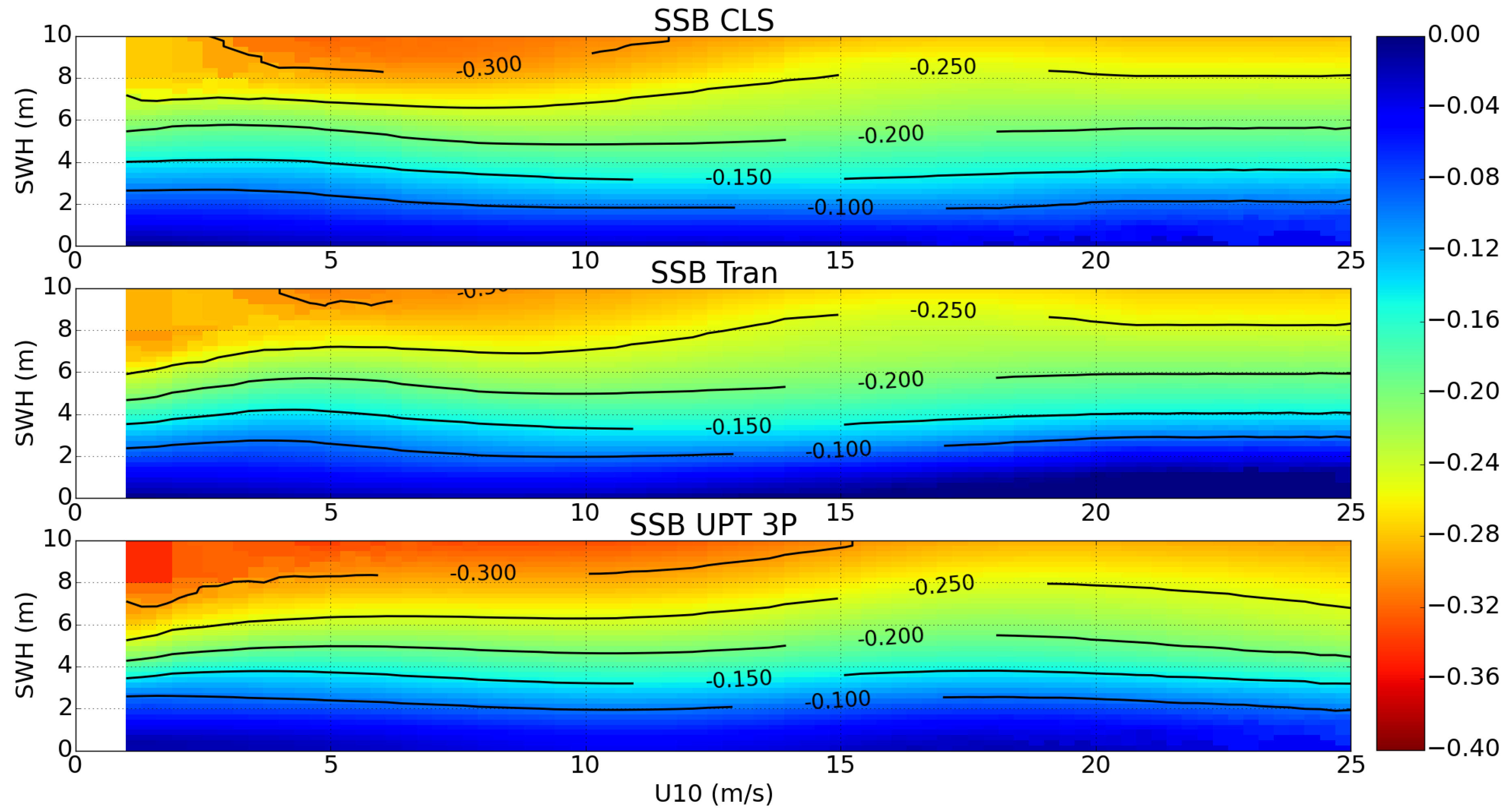
3.2. SSB Modeling Procedures and Design

The direct method of sea state impacts was implemented in order to give a reliable SSB estimation input for the final model. The method is characterized by the computation of the SSH uncorrected for SSB and binned afterwards against altimeter U10 and SWH, by imposing a constant a priori mean sea level at each altimeter observation location, thus producing a Sea Surface Height Anomaly (SSHA) uncorrected for SSB. For this work, the global high resolution mean sea surface DTU13 from DTU Space [25], available in RADS, was adopted. The direct method was implemented with a bin width of 0.25 m/s in U10 and 0.25 m in SWH, following the same procedure described by [9]. Instead of a bin-averaged computation, a more robust parameter of central tendency like the median was chosen, thus allowing lower discrepancies in the extremes of SSHA domain.

A training dataset estimated for the first 3 years of Jason-1 (first 112 cycles) produced a raw SSHA output with 3821 bins, which had to be subjected to a preliminary assessment in order to improve the bins quality for subsequent application. After evaluation, it was decided to discard all bins with less than 300 measurements, thus reducing the initial output to 2332 bins, i.e., 60% of the initial number.

Table 2. Binning summary statistics with all parameters and metrics considered per bin. 2332 bins were validated to estimate a training dataset considering the first 3 years of Jason-1 mission. Bins with less than 300 measurements were discarded.

Name (Statistic) (Units)	n	Mean	Std	Median	Min	Max
SWH (median) (m)	2332	4.88	2.39	4.87	0.40	9.88
U10 (median) (m/s)	2332	11.96	5.73	11.88	1.22	22.62
SSHA (mean) (m)	2332	−0.17	0.08	−0.18	−0.32	0.00
SSHA (median) (m)	2332	−0.17	0.07	−0.18	−0.32	−0.01
SSHA (std) (m)	2332	0.12	0.01	0.12	0.09	0.21
SSHA (mad) (m)	2332	0.09	0.01	0.09	0.06	0.12
SSHA (npoints)	2332	n.a.	n.a.	n.a.	300	673359
Tz G03 (median) (s)	2332	8.25	1.95	8.59	2.77	11.73

shows important information about the model predictors (SWH, U10, TzG03) and the response that will be modeled, the median of SSHA. The summary statistics does not reflect the real differences between the median and the mean of SSHA, but a preliminary assessment showed that the median is less affected by the points with extremely low values of SWH. Also from the table below, it is already possible to have a better idea of the final SSB that will be modeled looking at the SSHA median with a range between −0.32 m and −0.01 m.

After analyzing the behavior of each predictor with the response, it was necessary to control the weight of each bin in the model design. This weighting procedure uses the number of points and the standard deviation associated to each bin and applies an increasing and decreasing ramp function ($1-e^{-x}$ and $e^{-x}$) based on natural exponential functions. Diagnostic tests based on histograms, residual plots and fitted values vs their response, had to be performed for convergence analysis of the smoothness selection optimization and to study the impacts of the fitting procedure on the results. After this step, a robust method to identify and eliminate existing outliers based on residuals analysis was applied, where the predicted values with associated residuals larger than 2 standard deviations (2σ), were considered outliers and removed accordingly. After this procedure, the initial dataset of 2332 bins decreased to 2174 bins, i.e., a reduction sample of 7%. It was observed a good agreement between the fitted values and response, with an extremely low dispersion for the entire analyzed domain and a normal distribution without skewness, indicating also a good agreement between the fitted values and the response.

In order to evaluate the third predictor impact in the final response, two approaches were considered for the checking assessment and to choose the best candidate of SSB model design.

• ${\text{SSB}}_{2P}={\beta }_0+f_1\left(\mathrm{SWH}\right)+f_2\left(U10\right)$
• ${\text{SSB}}_{3P}={\beta }_0+f_1\left(\mathrm{SWH}\right)+f_2\left(U10\right)+f_3\left(T_{z}G03\right)$

where $f_1$, $f_2$ and $f_3$ are the smooth functions indicating the individual impact of each predictor. To accomplish this selection, the methodology for choosing the best model performance was based in a number of statistical parameters presented in

Table 3. Overall statistical performance of the two tested approaches. A verified reduction of Akaike Information Criterion (AIC) and Generalized Cross Validation (GCV) from SSB_3P relative to SSB_2P, indicating a more optimized model performance when a third predictor is considered. Coefficient of determination (R²) and Analysis of Variance (ANOVA) reinforce the same assumption.

Model	AIC	GCV	R2	ANOVA Pr (>Chi)
1. SSB2P	−13470	18.1 × 10−5	0.9668	-
2. SSB3P	−17067	38.8 × 10−6	0.9929	2.2 × 10−16

: Akaike Information Criterion (AIC), Generalized Cross Validation (GCV), coefficient of determination ($R^2$) and Analysis of Variance (ANOVA). Comparing the performance of the two tested models, ${\text{SSB}}_{3P}$ appears to be the one that fits better the response with lower AIC and GCV, and higher deviances explained by $R^2$. The ANOVA test results show low P values between the models, which indicates that we can reject the null hypothesis and consider statistical significant incorporating more nonlinear effects for model improvement.

Due to the interdependencies between predictors, where U10 = $f\left({\sigma }^0\right)$ and $T_{z}G03$ = $f(SWH,{\sigma }^0)$, both $SS{B}_{2P}$ and $SS{B}_{3P}$ are established using only two satellite derived products (SWH and ${\sigma }^0$), but the addition of $T_{z}G03$ can be considered as a mediator term, thus adding more information to the model on how SWH and ${\sigma }^0$ correlate. The impact of $T_{z}G03$ is evaluated in terms of how this predictor explains the variability of the model response traduced by the SSB estimation.

Figure 5 shows a comparative analysis, for the same training dataset, between the SSHA after evaluation, the established SSB models (SSB CLS and SSB Tran), a simple linear empirical model using a first order predictor, and the two fitted models designed with two and three predictors (SSB_UPT_2P and SSB_UPT_3P).

In Figure 5, it is possible to observe some noise in the fringes of SSHA for ocean swell regions (high SWH and low U10) and young seas regions (low SWH and high U10) that had to be smoothed by the final model. A first order SSB parametrization computed by −3.8% of SWH shows what should be the SSB linear behavior in the domain considered and its strong dependence with respect to wave height. The two predictor model SSB_UPT_2P shows a clear agreement with SSB CLS, even in those regions characterized with high wave heights and wind speeds, indicating an appropriate choice of the procedures taken for model design and strategies adopted. A good agreement can also be observed between SSB_UPT_3P and the 3-dimensional model SSB Tran, showing the contribution of $T_{z}G03$ in explaining the SSB variability for regions with U10 < 5 m/s, clearly demonstrating the impact of this third predictor when compared with SSB_UPT_2P.

3.3. Model Testing with New SSB Predictions

In order to better evaluate SSB_UPT_3P performance, new predictions were produced for a testing dataset, giving a new set of values not used to train the model and ranging between cycles 150–260 of Jason-1. Figure 6 shows that similar results were obtained for SSB_UPT_3P when computed for a testing dataset, revealing a well trained procedure with 3 year data from the first 112 cycles. There is a slight overestimation when compared with SSB Tran, especially in the region where SWH > 6 m and 5 m/s < U10 < 10 m/s, but not verified when compared with SSB CLS. The impact of $T_{z}G03$ is again verified and traduced by the isolines shrinkage observed in low wind regions with SSB predictions varying almost 15 cm for 2 m < SWH < 7 m which is consistent again with the SSB Tran model.

A spatial statistic assessment was performed with scaled Sea Level Anomalies (SLA) variance differences based on collinear analysis, where the satellite data were binned in lat-lon squares of 4° by 4°. The scaled SLA variance differences are shown to better illustrate the impact of different SLAs relative to the region variability, and are determined by $S=[(var\left(SL{A}_1\right)-var\left(SL{A}_2\right))/var\left(SL{A}_1\right)]\times 100$. Figure 7 represents a global assessment of the scaled SLA differences for SLAs computed with SSB_UPT_3P and SSB Tran for the entire phase A of Jason-1 mission, thus showing better performances of SSB_UPT_3P (blue) in the swell regions of Pacific and Atlantic oceans, but a poorer behavior especially in the North Indian ocean, Indonesia region and west side of South America. This result could be explained due to a verified underestimation of $T_{z}G03$ for some seasons in these regions when compared with WW3.

Table 4. Summary statistics of the SLA computed with different SSB models for the whole phase A of Jason-1 mission, where conformity between the proposed model SSB_UPT_3P and the established SSB approaches is verified. Last column shows each SSB correction impact on SLA variance reduction. All values in cm with exception to varSLA which is in cm².

Model	Mean	Std	Min	Max	varSLA ↓
SSB 1P	−9.96	5.04	−38.0	0.0	24.397
SSB CLS	−11.15	4.74	−32.1	−0.4	25.101
SSB Tran	−10.69	4.67	−30.9	3.7	25.117
SSB UPT 3P	−10.87	5.10	−34.8	-1.2	25.265

resumes the statistical parameters of the different SSB models for the whole phase A mission of Jason-1 with the corresponding performance in SLA variance reduction. The last column presents each SSB correction impact on SLA variance reduction with respect to the scenario when no SSB correction is applied. The measure of central tendency shows conformity between the standard models and the proposed one. All three approaches have equivalent SSB standard deviations in explaining the response variability, which is consistent with the estimated variance reduction of SLA verified in some geographical regions with the SLA computed with SSB_UPT_3P.

Even though the favorable performance of SSB_UPT_3P in estimating a correction in line with the satandard SSB models, some differences are still verified specially in the edges of SWH-U10 domian. The results shown in Figure 7 and Table 4 could not be only explained by the fact that SSB_UPT_3P is using a third predictor not implemented in SSB Tran and SSB CLS, but instead by the different statistical techniques used. Standard models use the same local-linear kernel smoothing approach, which can produce different impacts on model predictions, specially at the edges of SWH-U10 domain with more variability. However, the smoothing splines technique, being a direct basis expansion of the original data, is flexible enough by choosing the number and locations of the knots used in those regions that could change rapidly.

4. Discussion

The presented work shows a new approach for SSB modeling based on three predictors derived only by altimetric information.

A preliminary assessment was made to evaluate the performance of two different mean wave period algorithms when compared with WW3 numerical wave model, leading to the selection of the proposed algorithm by [14] due to its simplicity, ease of implementation, and efficiency in estimating the mean wave period for different ocean regimes and seasons.

The direct estimation method proposed by [9] was implemented to obtain a reliable SSHA input for modeling. Despite the good results, the method produces some noisy estimations in the fringes of SWH-U10 domain, needing to be tweaked by weighting techniques and bins cleaning procedures before use.

The method shows a good estimating performance with fewer cycles as input, suggesting that is possible to estimate a reliable SSB correction with a smaller training dataset, an important feature for the computation of SSB models for future missions, during the initial period of the mission.

The adopted SSB modeling approach with penalized spline smoothing embedded in a general framework provided by GAMs, reveals to be a straightforward modeling tool with a good compromise between flexibility, reduced computational requirements and accuracy of results. This technique is also expandable to accommodate interactions between explanatory variables, providing a deeper knowledge on how different predictors correlate together.

Two SSB models designs (SSB_UPT_2P, SSB_UPT_3P) were tested and subjected to a careful assessment of quality checking and residual analysis. SSB_UPT_3P exhibits a good performance when compared with the established SSB models (SSB CLS, SSB Tran), with predictions in line with [11] 3-dimensional model, especially for swell ocean regions. Although there is a total SLA variance reduction of almost 15 mm² for all the phase A of Jason-1, a spatial mixed performance in SLA variance was also verified, with ranges between 3%–4% of SLA variance reduction and a 2%–3% of SLA variance increase when compared with SSB Tran model.

5. Conclusions

This new technique aims to be a fast and reliable approach for SSB computation, combining three nonlinear predictors in a model design provided by an effectively modeling approach as the smoothing splines integrated with Generalized Additive Models. The third predictor represented by the selected mean wave period algorithm TzG03, has a low impact on SSB when compared with SWH and U10, but has the role of a mediator parameter influencing the model input with the interaction between SWH and U10. The achieved results show a clear improvement when the model gathers this extra information about the sea state conditions. The proposed approach was designed with simplicity and reliability in mind, despite some detected deficiencies of the used mean wave period algorithm when compared with WW3, it has been proven that it has a good performance for a wide range of ocean conditions, providing the best compromise between simplicity and reasonable results. While the simplest approach was privileged, this choice does not eliminate the possibility of implementing alternative algorithms in the future.

As a final note, it should be emphasized that it is not the aim of the proposed method to be better than the established SSB models, but instead, to provide an alternative procedure for a reliable model, in line with the best current models, easy to handle and control, flexible enough to be adapted for other altimetric missions, in particular for forthcoming missions.

References

1. Melville, W.K.; Stewart, R.H.; Keller, W.C.; Kong, J.A.; Arnold, D.V.; Jessup, A.T.; Loewen, M.R.; Slinn, A.M. Measurements of electromagnetic bias in radar altimetry. J. Geophys. Res. 1991, 96, 4915–4924. [Google Scholar] [CrossRef]
2. Chelton, D.B.; Ries, J.C.; Haines, B.J.; Fu, L.L.; Callahan, P.S. Satellite altimetry, in Satellite Altimetry and Earth Sciences edited by L. Fu and A. Cazenave. Int. Geophys. Ser. 2001, 69, 1–31. [Google Scholar]
3. Ghavidel, A.; Schiavulli, D.; Camps, A. Numerical Computation of the Electromagnetic Bias in GNSS-R Altimetry. IEEE T. Geosci. Remote 2006, 54, 489–498. [Google Scholar] [CrossRef]
4. Born, G.H.; Richards, M.A.; Rosborough, G.W. An empirical determination of the effects of sea state bias on SEASAT altimetry. J. Geophys. Res. 1982, 87, 3221–3226. [Google Scholar] [CrossRef]
5. Gaspar, P.; Le Traon, P.; Zanife, O. Estimating the sea state bias of the TOPEX and POSEIDON altimeteres from crossover differences. J. Geophys. Res. 1994, 99, 24981–24994. [Google Scholar] [CrossRef]
6. Gaspar, P.; Florens, J. Estimation of the sea state bias in radar altimeter measurements of sea level: Results from a new nonparametric method. J. Geophys. Res. 1998, 103, 803–814. [Google Scholar] [CrossRef]
7. Gaspar, P.; Labroue, S.; Ogor, F. Improving Nonparametric Estimates of the Sea State Bias in Radar Altimeter Measurements of Sea Level. J. Atmos. Ocean. Technol. 2002, 19, 1690–1707. [Google Scholar] [CrossRef]
8. Feng, H.; Yao, S.; Li, L.; Tran, N.; Vandemark, D.; Labroue, S. Spline-Based Nonparametric Estimation of the Altimeter Sea-State Bias Correction. IEEE Geosci. Remote Sens. Lett. 2010, 7, 577–581. [Google Scholar] [CrossRef]
9. Vandemark, D.; Tran, N.; Beckley, B.; Chapron, B.; Gaspar, P. Direct estimation of sea state impacts on radar altimeter sea level measurements. Geophys. Res. Lett. 2002, 29, 2148. [Google Scholar] [CrossRef]
10. Tran, N.; Vandemark, D.; Chapron, B.; Labroue, S.; Feng, H.; Beckley, B.; Vincent, P. New models for satellite altimeter sea state bias correction developed using global wave model data. J. Geophys. Res. 2006, 111. [Google Scholar] [CrossRef]
11. Tran, N.; Vandemark, D.; Labroue, S.; Feng, H.; Chapron, B.; Tolman, H.L.; Lambin, J.; Picot, N. Sea state bias in altimeter sea level estimates determined by combining wave model and satellite data. J. Geophys. Res. 2010, 115, 1–7. [Google Scholar] [CrossRef]
12. Davies, C.G.; Challenor, P.G.; Cotton, P.D. Measurement of wave period from radar altimeters. Ocean wave measurement and analysis. Am. Soc. Civ. Eng. 1997, 819–826. [Google Scholar]
13. Hwang, P.; Teague, W.; Jacobs, G.; Wang, D. A statistical comparison of wind speed, wave height, and wave period derived from satellite altimeters and ocean buoys in the Gulf of Mexico region. J. Geophys. Res. 1998, 103, 10451. [Google Scholar] [CrossRef]
14. Gommenginger, C.P.; Srokosz, M.; Challenor, P.; Cotton, D. Measuring ocean wave period with satellite altimeters: A simple empirical model. Geophys. Res. Lett. 2003, 30, 2150. [Google Scholar] [CrossRef]
15. Quilfen, Y.; Chapron, B.; Collard, F.; Serre, M. Calibration/Validation of an Altimeter Wave Period Model and Application to TOPEX/Poseidon and Jason-1 Altimeters. Mar. Geod. 2004, 27, 535–549. [Google Scholar] [CrossRef]
16. Mackay, E.; Retzler, C.H.; Challenor, P.; Gommenginger, C.P. A parametric model for ocean wave period from Ku band altimeter data. J. Geophys. Res. 2008, 113, 1–16. [Google Scholar] [CrossRef]
17. Govindan, R.; Kumar, R.; Basu, S.; Sarkar, A. Altimeter-derived ocean wave period using genetic algorithm. IEEE Geosci. Remote Sens. Lett. 2011, 8, 354–358. [Google Scholar]
18. Scharroo, R. RADS Version 3.1 User Manual and Format Specification; 2012. [Google Scholar]
19. Scharroo, R. RADS Version 4.2.4 User Manual; 2016. [Google Scholar]
20. Chelton, D. The sea state bias in altimeter estimates of sea level from collinear analysis of TOPEX data. J. Geophys. Res. 1994, 99, 24995–25008. [Google Scholar] [CrossRef]
21. Scharroo, R.; Lillibridge, J. Non-Parametric Sea-state Bias Models and Their Relevance to Sea Level Change Studies. In Proceedings of the ENVISAT/ERS Symposium, Salzburg, Austria, 6–10 September 2004.
22. Caires, S.; Sterl, A.; Gommenginger, C.P. Global ocean mean wave period data: Validation and description. J. Geophys. Res. 2005, 110, 1–12. [Google Scholar] [CrossRef]
23. James, G.; Witten, D.; Hastie, T.; Tibshirani, R. An Introduction to Statistical Learning with Applications in R; Springer Texts in Statistics; Springer: New York, NY, USA, 2014. [Google Scholar]
24. Wood, S. Generalized Additive Models: An introduction with R; Chapman & Hall/CRC Texts in Statistical Science; CRC Press: Florida, FL, USA, 2006; Volume 62. [Google Scholar]
25. Andersen, O.; Knudsen, P.; Stenseng, L. The DTU13 MSS (Mean Sea Surface) and MDT (Mean Dynamic Topography) from 20 Years of Satellite Altimetry; Springer: Berlin, Germany, 2015. [Google Scholar]
Figure 1. Flowchart diagram with the main steps of the model design. Starting on the left side, with altimetric data input, new parameters computation and selection criteria for binning procedure, and finishing on the right with strategies used for SSB modulation and predictions.
Remotesensing 08 00576 g001
Figure 2. Statistical analysis of mean wave period algorithms G03, Q04 and the Tz derived from numerical wave model WW3 (from left to right), for the first 50 cycles of Jason-1. All plots displaying the number of validated measurements, mean absolute error (MAE), root mean square error (RMSE) and correlation between measurements.
Remotesensing 08 00576 g002
Figure 3. Statistical analysis of mean wave period algorithms G03, Q04 and the Tz derived from numerical wave model WW3 (from left to right), for the first 50 cycles of Jason-1 with swell ratio < 0.9 activated.
Remotesensing 08 00576 g003
Figure 4. Global correlation between TzG03 and TzWW3. Data were binned in lat-lon squares of 4° by 4° with swell ratio (SR) deactivated. Largest correlations are found at high latitudes, predominantly in swell ocean regions.
Remotesensing 08 00576 g004
Figure 5. Training dataset of Sea Surface Height Anomaly (SSHA) (top left) and different SSB models outputs for SWH-U10 domain considering the same datataset. A linear empirical model using only one predictor computed by −3.8% of SWH (top right), the two established SSB models (SSB CLS and SSB Tran on middle left and right, respectively) currently available in Jason-1 mission, and the two SSB models designed on this study (bottom left and right).
Remotesensing 08 00576 g005
Figure 6. SSB performances for a testing dataset ranging between Jason-1 cycles 150-260 in SWH-U10 domain. From top to bottom, SSB CLS approach using the two classic predictors (SWH and U10), SSB Tran modulation using the same previous predictors, but adding the extra mean wave period information derived from WW3, and the proposed model design SSB_UPT_3P with TzG03 acting as a mediator parameter, interacting with SWH and U10.
Remotesensing 08 00576 g006
Figure 7. Percentage of scaled sea level anomalies (SLA) variance differences between SLAs computed with SSB_UPT_3P and SSB Tran. Blue squares represent regions with a decrease in SLA variance computed with the proposed SSB model with respect to SSB Tran. Red squares indicate regions where an increase in SLA variance from SSB UPT 3P relative to the SLA variance computed with SSB Tran is observed.
Remotesensing 08 00576 g007