Diagnosing Horizontal and Inter-Channel Observation Error Correlations for SEVIRI Observations Using Observation-Minus-Background and Observation-Minus-Analysis Statistics

Abstract

It has been common practice in data assimilation to treat observation errors as uncorrelated; however, meteorological centres are beginning to use correlated inter-channel observation errors in their operational assimilation systems. In this work, we are the first to characterise inter-channel and spatial error correlations for Spinning Enhanced Visible and Infrared Imager (SEVIRI) observations that are assimilated into the Met Office high-resolution model. The errors are calculated using a diagnostic that calculates statistical averages of observation-minus-background and observation-minus-analysis residuals. This diagnostic is sensitive to the background and observation error statistics used in the assimilation, although, with careful interpretation of the results, it can still provide useful information. We find that the diagnosed SEVIRI error variances are as low as one-tenth of those currently used in the operational system. The water vapour channels have significantly correlated inter-channel errors, as do the surface channels. The surface channels have larger observation error variances and inter-channel correlations in coastal areas of the domain; this is the result of assimilating mixed pixel (land-sea) observations. The horizontal observation error correlations range between 30 km and 80 km, which is larger than the operational thinning distance of 24 km. We also find that estimates from the diagnostics are unaffected by biased observations, provided that the observation-minus-background and observation-minus-analysis residual means are subtracted.

1. Introduction

To provide an accurate forecast, numerical weather prediction (NWP) models must be evolved from accurate initial conditions. Since the true state of the atmosphere is unknown, estimates of these initial conditions must be determined using information from both previous forecasts and from observations . Using the technique of data assimilation, the observations and previous forecasts, known as backgrounds, are weighted by their respective errors and combined to provide a best guess of the state, known as the analysis. Hence, it is important to have an accurate representation of the background and observation error statistics in the assimilation.

The observation error can be attributed to a number of sources. The instrument, or measurement, error is uncorrelated for most instrument types; however, correlated errors are likely to arise from pre-processing errors, errors in the operator that maps between model and observation space and representativity errors. Representativity errors arise when the observations can resolve scales that the model can not [1,2]. The instrument error is often known and well understood, but the contribution from the other error sources is complex and information about them is limited. However, errors arising from the observation operator uncertainty in the context of fast radiative transfer modeling have been considered by e.g., [3,4]. Until recently, in operational data assimilation, the observation errors have been assumed uncorrelated and processes such as variance inflation, observation thinning and ‘superobbing’ have been used to either reduce the correlated error or account for the unknown correlations. To improve the accuracy of the analysis and the number of observations assimilated, it is necessary to understand and account for the full, potentially correlated, observation error statistics. These error statistics cannot be calculated directly so must be estimated statistically. Desroziers et al. [5] proposed a diagnostic that provides an estimate of the observation error covariance matrix by considering the statistical average of observation-minus-background and observation-minus-analysis residuals. In theory, it relies on the use of exact background and observation error statistics in the assimilation; however, it has been used successfully in simple model experiments in both variational [6] and ensemble [7,8] data assimilation systems and to estimate time varying observation errors [9] when the assimilated error statistics are incorrect. Furthermore, recent theoretical work provides a detailed insight on how results from the diagnostic can be interpreted when the incorrect background and observation error statistics are used in the assimilation [10]. In addition, an improved estimate of the error statistics may be obtained if successive iterations of the diagnostic are applied [5,11], although this iteration procedure is often not possible in operational systems that are currently unable to assimilate observations with correlated error.

An important set of observations used in NWPs are those observed by satellite instruments. Inter-channel correlations have been calculated for observations from satellite instruments such as the Atmospheric Infrared Sounder (AIRS) and Infrared Atmospheric Sounding Interferometer (IASI) using the Desroziers et al. diagnostic [12,13,14,15,16]. The literature shows that inter-channel observation errors are correlated and that including these errors in the assimilation leads to improved analysis accuracy, better forecast skill score and the inclusion of more observation information content [6,16,17,18,19]. As a result, the assimilation of correlated inter-channel errors for IASI observations is now operational at the Met Office. The benefit seen by including correlated inter-channel errors provides motivation to calculate observation error statistics for other satellite instruments. As well as providing potential benefit to the assimilation, the calculation of both the inter-channel and spatially correlated errors may provide information that allows better use of the observations, either by a reduction in thinning, an optimisation of channel selection or by highlighting areas where the observation operator may be improved. In this work, we are the first to use the Desroziers et al. method to calculate inter-channel error correlations for observations obtained using the Spinning Enhanced Visible and InfraRed Imager (SEVIRI) [20]. Different from previous work estimating inter-channel error covariances using this method, we demonstrate the variation of results across the geographical domain and the enhanced understanding that this can bring. We also consider whether the SEVIRI observation errors are spatially correlated. We are not aware of any previous work in the literature calculating spatial correlations for satellite data using this method, although we have done this for ground-based weather radar [21].

Our new results show that all the estimated error variances are lower than those used operationally. For the inter-channel correlations, we find that upper level water vapour channels have strongly correlated errors as do the surface channels. We also consider how the inter-channel correlations vary across the domain. These results show that the inter-channel correlations for the surface channels are much stronger in coastal areas. We find that this is the result of mixed pixel (mixed surface type) observations being assimilated. For the horizontal errors, we find that the correlation length scale is larger than the operational thinning distance, with the length scales ranging between 50 km and 80 km dependent on the observation channel. Considering the horizontal correlation for sea-only observations increases the correlation length scale and suggests that errors associated with the mixed pixel observations have a different structure to the errors associated with the sea-only pixels. Accounting for the correlated SEVIRI errors in the data assimilation is expected to be of benefit to the analysis.

Whilst calculating these results, we find that the estimates from the diagnostics are unaffected by a bias in the observations, providing that the means of the observation-minus-background and observation-minus-analysis residuals are subtracted to make the estimation unbiased.

This paper is organised as follows. In Section 2, we describe the Desroziers et al. method that we use to calculate observation error statistics; we also describe the SEVIRI observations and their model representation. The experimental design is described in Section 3. The estimated inter-channel and horizontal error correlation results are presented in Section 4. Finally, we conclude in Section 5.

2. Methodology

2.1. The Diagnostic of Desroziers et al. (2005)

In data assimilation, observations, $\mathbf{y}\in {\mathbb{R}}^{N^p}$, are combined with a model prediction of the state, the background ${\mathbf{x}}^b\in {\mathbb{R}}^{N^m}$, that is often determined by a previous forecast. Both observations and background contain errors; these are described by the background and observation error covariance matrices, $\mathbf{B}\in {\mathbb{R}}^{N^m\times N^m}$ and $\mathbf{R}\in {\mathbb{R}}^{N^p\times N^p}$, respectively. These covariances are used to weight the background and observations when they are combined to obtain a best estimate of the state ${\mathbf{x}}^a\in {\mathbb{R}}^{N^m}$, known as the analysis. The analysis provides a set of initial conditions that can be evolved forward in time using the non-linear model, $\mathcal{M}$, to provide a background at the next assimilation time, ${\mathbf{x}}^b=\mathcal{M}\left({\mathbf{x}}^a\right)$.

The error covariances associated with the observations cannot be calculated exactly, and, therefore, they must be estimated statistically. One method that provides an estimate of the observation errors is presented in [5]. This diagnostic determines an estimate of the observation error covariance matrix by taking the statistical expectation of the observation-minus-background and observation-minus-analysis residuals. The background residual, also known as the innovation,

$${\mathbf{d}}_b^o=\mathbf{y}-\mathcal{H}\left({\mathbf{x}}^b\right),$$

(1)

is the difference between the observation, $\mathbf{y}$, and the mapping of the forecast vector, ${\mathbf{x}}^b$, into observation space by the observation operator $\mathcal{H}:{\mathbb{R}}^{N^p}\to {\mathbb{R}}^{N^m}$. Replacing the forecast vector with the analysis vector calculated using Equation (1), ${\mathbf{x}}^a$, results in the analysis residual,

$$\begin{array}{ccc}\hfill {\mathbf{d}}_a^o& =& \mathbf{y}-\mathcal{H}\left({\mathbf{x}}^a\right),\hfill \end{array}$$

(2)

$$\begin{array}{ccc}& \approx & \mathbf{y}-\mathcal{H}\left({\mathbf{x}}^b\right)-\mathbf{HK}{\mathbf{d}}_b^o,\hfill \end{array}$$

(3)

where $\mathbf{K}={\mathbf{BH}}^T{({\mathbf{HBH}}^T+\mathbf{R})}^{-1}$ is the gain matrix and $\mathbf{H}$ is the linearised observation operator, linearised about the current state.

Assuming that the forecast and observation errors are uncorrelated, the statistical expectation of the outer product of the analysis and background residuals results in

$$E\left[{\mathbf{d}}_a^o{{\mathbf{d}}_b^o}^T\right]\approx \mathbf{R}.$$

(4)

This equation produces the exact observation error covariance matrix if the observation and background error statistics used in the assimilation are exact. If the incorrect background and observation error statistics are used in the assimilation, then the theoretical work of [10] provides insight on how to interpret the results from the diagnostic. In particular, these results suggest that when correlated observation errors are treated as uncorrelated in the assimilation, the diagnostic will underestimate the observation error correlation length-scale. A further issue with the diagnostic is that it is not guaranteed to yield a symmetric matrix. Therefore, the matrix must be symmetrised before it can be used in the assimilation.

The current statement of the diagnostic assumes that the observation-minus-background and observation-minus-analysis residuals are unbiased. Operationally assimilated observations are bias corrected so it is unlikely that observation-minus-background and observation-minus-analysis will be biased. However, when calculating the diagnostic, we subtract the mean residual values (as in Equation (4.3) of [6]) to ensure our result is unbiased.

The diagnostic has a number of limitations; however, with careful interpretation of the results, it can be used to provide valuable information not only on the observation error structure itself, but also on how the observations may be best used in the assimilation.

2.2. The Met Office UKV Model and 3D Variational Assimilation Scheme

The Met Office high resolution convection permitting model, the UKV, is a variable resolution model that covers the UK [22,23,24,25]. The horizontal grid has a 1.5 km fixed resolution on the interior surrounded by a variable resolution grid, which increases smoothly in size to 4 km. The global model provides boundary conditions for the UKV, which are downscaled to the 4 km boundary resolution; the variable resolution grid allows the boundary conditions to spin up before reaching the fixed interior grid. The initial conditions are provided from a limited-area version of the Met Office 3D variational assimilation scheme (3D-VAR) [26,27], which has an analysis grid of 3 km and uses an incremental approach [28]. In the assimilation, the 70 vertical model levels are determined using an adaptive mesh. This allows the accurate representation of boundary layer structures [29,30].

The climatological background-error covariance statistics used in this study are those that were used in the operational Met Office UKV system in January 2013. The Met Office’s covariance calibration and diagnostic tool for covariances and VAR transforms (CVT) have been used to supply these background error covariance statistics. Here, an NMC method [31] has been applied to (T+6 h)-(T+3 h) forecast differences to diagnose a variance and correlation length scale for each vertical mode.

2.3. SEVIRI Observations

The Spinning Enhanced Visible and Infrared Imager (SEVIRI) on board the Meteosat Second Generation satellite produces observations of radiances at the top of the atmosphere from 12 different spectral channels every 15 min at a 3 km spatial resolution [32]. Clear sky SEVIRI radiances from five channels, detailed in

Table 1. SEVIRI Observation error variances.

Channel	Channel	Channel	Assimilated over
Number	Wavelength (μm)	Description	Land/Sea/Low Cloud
5	6.2	Upper level water vapour (humidity)	✔/✔/✔
6	7.3	Upper level water vapour (humidity)	✔/✔/✘
7	8.7	Surface (temperature)	✘/✔/✘
9	10.8	Surface (temperature)	✘/✔/✘
10	12.0	Surface (temperature)	✘/✔/✘

, have been assimilated into the Met Office NWP system since 2008 [33]. The assimilation of radiances over regions of low cloud from Channel 5 was introduced in 2013, as this helps to constrain the humidity in the mid- and upper-troposphere in the UKV model [34].

Before being assimilated, the SEVIRI observations are pre-processed using the Autosat system [35,36] where additional cloud masking is applied. A 1D variational assimilation scheme (1D-VAR) retrieval system is also used to quality control the observations. A bias correction, as described in [37], is applied to all observations before they are used in the assimilation. Finally, for operational assimilation, the data are thinned to a horizontal resolution of 24 km to reduce the observation error spatial correlations. The remaining observations are assigned an error variance that is used in calculating the 3D-VAR cost function in the assimilation. The assigned error variances for each channel, presented in

Table 2. SEVIRI Observation error variances.

Case	Channel 5	Channel 6	Channel 7	Channel 9	Channel 10
Operational	4.00	4.00	1.00	1.00	1.00
Inter-Channel Full Domain	1.19	0.40	0.19	0.16	0.20
Inter-Channel Land	1.17	0.44	-	-	-
Inter-Channel Coast	1.18	0.44	0.34	0.29	0.34
Inter-Channel Sea	1.19	0.39	0.07	0.06	0.09
Horizontal Full Domain	1.19	0.40	0.19	0.16	0.20
Horizontal Sea	1.19	0.39	0.07	0.06	0.09

, have been inflated in an attempt to account for the unrepresented correlated error. These inflated error variances are two orders of magnitude smaller than the value of the signal, which is O(10²)K.

For each SEVIRI observation, a simulated brightness temperature is calculated using the Radiative Transfer for Television Infrared Observation Satellites (TIROS) Operational Vertical Sounder (RTTOV) radiative transfer model (version 7) [38]. The RTTOV model maps the variables of surface air temperature, skin temperature, surface humidity and surface emissivity, as well as the vertical profiles of the first guess model fields of temperature and humidity into the observation space. These simulated brightness temperatures are strongly dependent on the input variables and their errors. For example, it has been shown that errors in the model skin temperature will introduce errors into the simulated brightness temperatures [39]. Further details on the limitations of the RTTOV model can be found in [38]. More accurate radiative transfer models are available [40], but are not suitable for operational NWPs for reasons of computational efficiency.

3. Experimental Design

In this work, we calculate both horizontal and inter-channel correlations for the SEVIRI observations. To calculate these correlations, we use archived observations and background data produced by the operational Met Office system from June, July and August 2013. The analysis fields are produced by rerunning the operational UKV assimilation scheme. To remove any of the model background points that may be affected by the boundary condition spin-up, we only consider observations that are located in the uniform grid area of the model.

As we are using an operational configuration for the assimilation, we are only able to calculate observation error correlations for the thinned SEVIRI data. As a result, when calculating the horizontal correlations, we are unable to consider correlations at a distance of less than 24 km. Experiments were also performed using an unthinned set of data to allow calculation of correlations at 5 km. These results are not presented here due to the suboptimality of the data assimilation scheme with unthinned observations. However, results are briefly discussed in the conclusions. The horizontal correlations are calculated separately for each of the five different channels. We determine the correlation length scale by considering where the correlation becomes insignificant (<0.2) [41]. We calculate inter-channel correlations using data across the entire domain; however, as channels 5 and 6 are available over both land and sea, we also investigate whether the correlations depend on surface type. We also calculate correlations over sub-domains of the model to consider how the correlations vary across the model domain.

Calculations using an initial set of operational data highlighted a large bias in the observations for Channel 5. Consequently, the bias correction was updated and a new assimilation was run over the same summer period. Here, we present results from the diagnostics using the bias corrected set of data. However, we note that, when using the biased data, results obtained from the diagnostics were qualitatively similar to those presented here. This important result highlights that, if the mean residual values are subtracted from the diagnostic, then the results are not sensitive to bias present in the original data.

4. Results

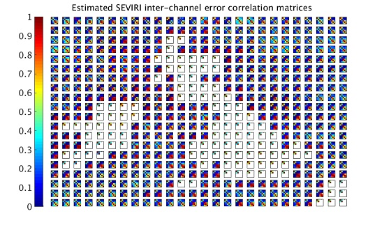
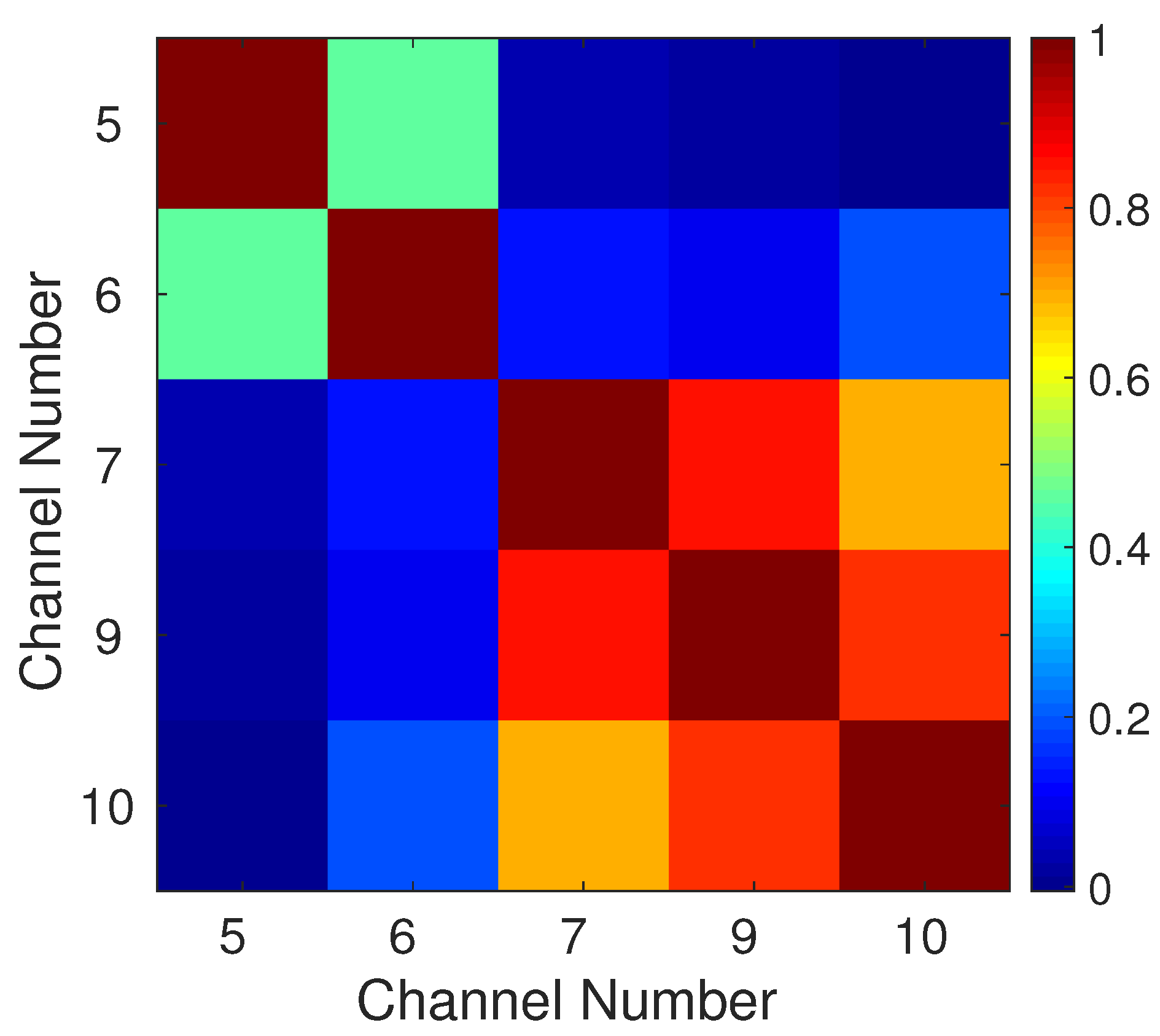
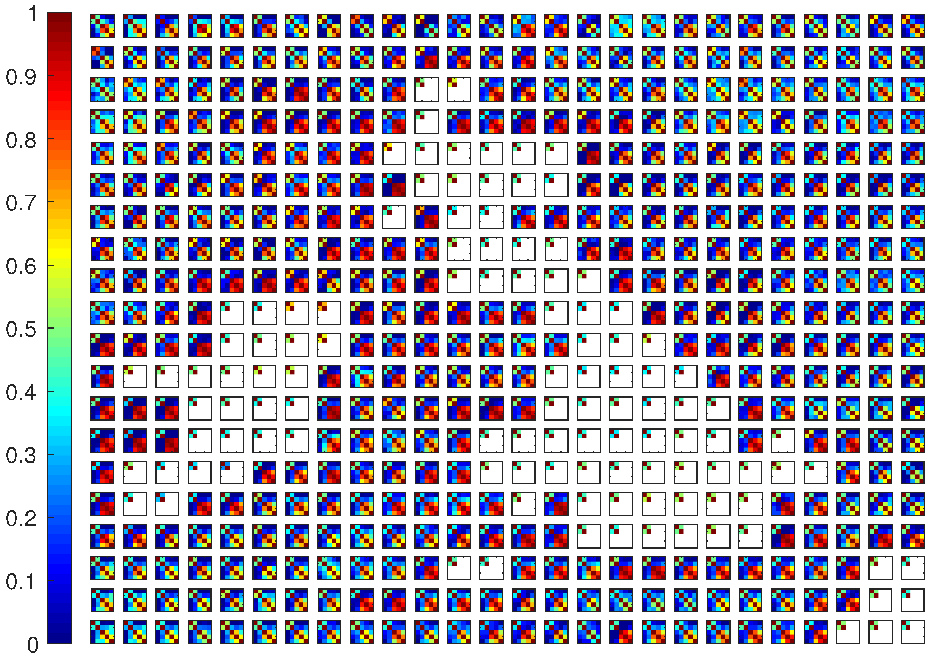
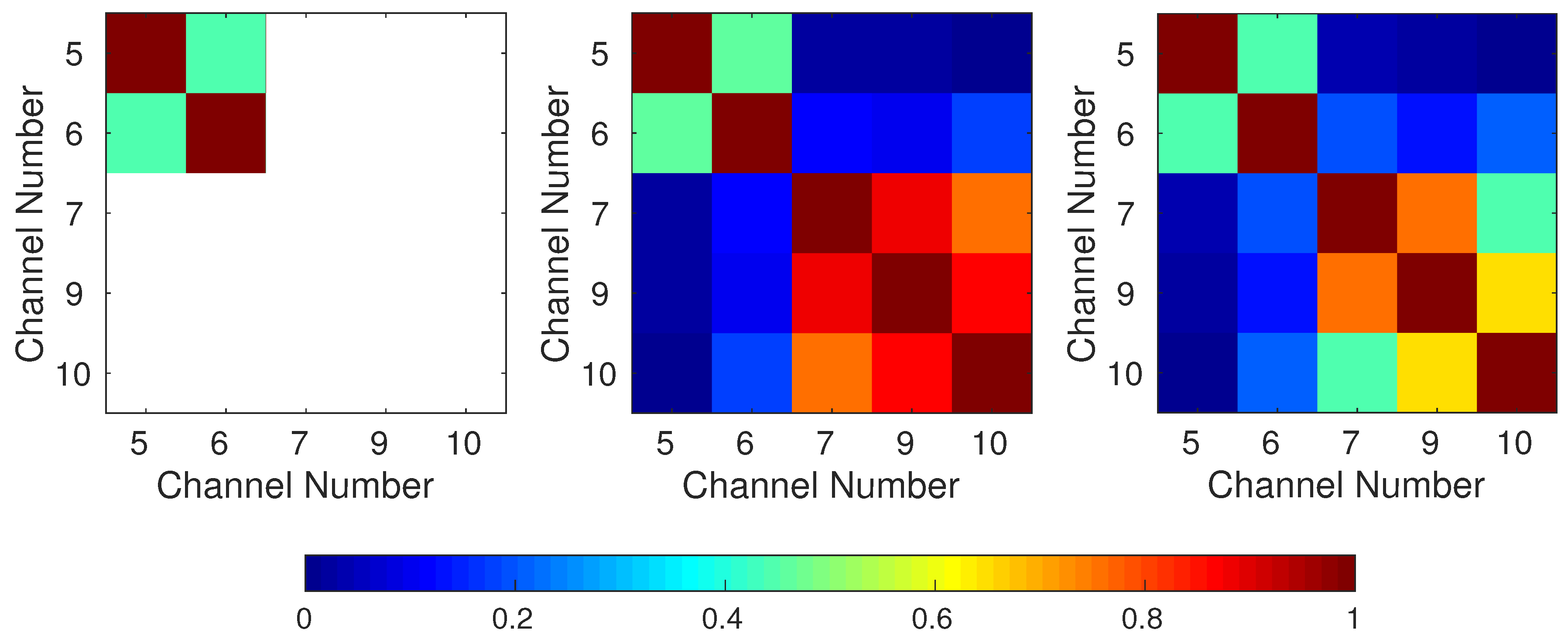
4.1. Inter-Channel Correlations

We first consider the estimated inter-channel covariance matrix using all available data across the entire domain. In Table 2, we present the estimated variances, along with the current operational variances (i.e., the variances used in calculating the 3D-VAR cost function in the assimilation). The estimated correlation matrix is plotted in Figure 1.

We see that the estimated variances for the upper level water vapour channels (5 and 6) are larger than those for the surface channels (7, 9 and 10). This is expected as the RTTOV scheme is less accurate at simulating radiances for the water vapour channels. The variance for Channel 5 is approximately three times larger than Channel 6; this is the result of the assimilation of Channel 5 observations over areas of low clouds, which are subject to larger errors in the observation operator.

For all channels, the estimated variances are much smaller than those currently used for the operational assimilation. This result can be attributed to the fact that (a) the assimilated observation errors are inflated in an attempt to account for the unrepresented correlated error and hence are larger than the actual observation errors; and (b) the result produced by the diagnostic is sensitive to the background and observation error statistics used in the assimilation. In the assimilation performed here, the observation error correlations are neglected, and it is assumed that the background error variances and correlation length scales are too long. In this case, the theoretical work of [10] suggests that the diagnostic will provide an under-estimate of the true observation error variance. The combination of inflated operational observation error variances, and the likelihood that the diagnostic produces under-estimated error variances suggests that the true error variance is between the operational and diagnosed variances. Since the operational error variances are inflated to compensate for neglecting the correlated errors, we hypothesise that the true error is likely to be closer to the estimated value.

In Figure 1, we plot the estimated inter-channel correlations. We see that upper level humidity channels 5 and 6 have significantly correlated errors, as do surface channels 7, 9 and 10. The correlations are likely caused by a combination of pre-processing, observation operator and representativeness error, and determining which portion of error can be attributed to each is complex. However, in this case, due to the high resolution of the model and the block structure of the correlations, it is reasonable to assume that it is the overlapping weighting functions used in the radiative transfer scheme that contribute most to the correlated error structure. Inter-channel correlation is also likely to be a result of erroneous values, such as sea surface temperature, that are passed through the RTTOV scheme since the simulated brightness temperatures are strongly dependent on RTTOV input variables and their errors. Given the expected gain of accounting for correlated errors in the assimilation (see Section 1), it may be beneficial to consider the use of these correlated SEVIRI errors in the assimilation.

We next considered whether the inter-channel observation error statistics varied spatially across the domain. The domain was divided into 0.5^o by 0.5^o degree sections and the inter-channel observation error statistics calculated for each sub-domain. As surface channels 7, 9 and 10 are only assimilated over sea, there are some sub-domains where there was no data available to estimate the error statistics. In Figure 2, we plot, for each channel, the estimated variance in each sub-domain. We find that the variance for the surface channels varies significantly over the domain, with larger variances over coastal areas. Figure 3 (correlation matrices for each sub-domain) also highlights that the correlations are influenced in coastal areas since the inter-channel correlations for the surface channels increase in these regions. It appears that the correlations for the upper level channels are not affected by surface type.

To clarify the impact that surface type had on the estimated observations error correlations, each sub-domain was then classified into one of three different surface categories—sea, land or coastal. The observation error statistics were then calculated for each surface type using data from the appropriate sections. Observation error variances for the different surface types are included in Table 2 and the correlations are plotted in Figure 4. From these results, we are able to conclude that the estimated error variance and correlations for the upper level water vapour channels (5 and 6) are not dependent on the surface type below the observation. However, the variance and correlations for the surface channels are dependent on whether the observation is over open ocean or a coastal area. We see that, for the surface channels, the variance and correlation is increased in coastal areas. The surface channels are only assimilated over sea due to the increase in standard deviation over land. However, in the operational assimilation, some ‘mixed pixel’ observations, where the footprint of the observation views a mixture of land and sea, were not being rejected by the quality control, and were being assimilated. The inclusion of the mixed pixel observations, with increased error standard deviations, are the cause of the increase in variance and correlation in the coastal areas. As, at present, there is no accurate way to simulate the mixed pixel observations, they should not be included in the assimilation. As a result, an improved quality control procedure to remove mixed pixel observations is being addressed within the Met Office. When investigating these results, we also considered whether they might have been caused by misregisration (which they were not). However, we note that the use of this diagnostic approach might be used to identify other errors such as misregistration.

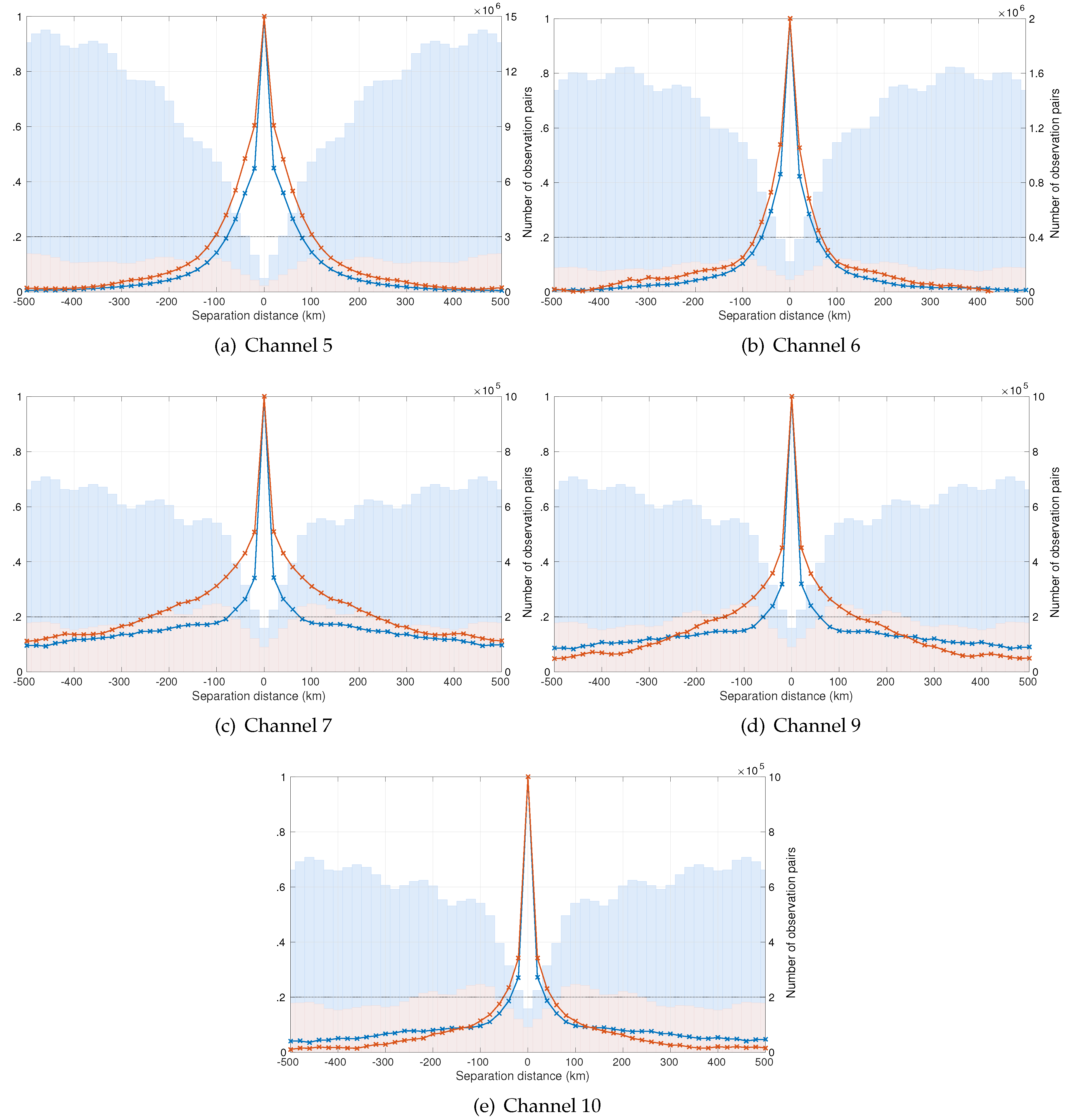
4.2. Horizontal Correlations

We next consider the horizontal observation error variances and correlations. We give the variances in Table 2 and see that these are equal to the full domain inter-channel variances; this is expected since the same data set is used to calculate the variance. We plot the horizontal correlations, along with the number of observation pairs used to calculate them, for each channel in Figure 5 (blue lines/bars). We see that the correlation structures for the upper level water vapour channels are similar (Figure 5a,b) with the correlation reducing smoothly and reaching zero by 500 km separation distance. However, the observations from Channel 5 have errors correlated with a longer length scale, 80 km, than observations from Channel 6 that have a correlation length scale of 65 km. It is possible that the larger correlation length scale for Channel 5 is caused by the assimilation of cloudy radiances from this channel. The surface channels (Figure 5c–e) also share a similar correlation structure with an initial sharp decrease in correlation before the correlation decays slowly, with some correlation, though not necessarily significant, still existing at the 500 km separation distance. Channel 7 has the longest correlation length scale of 75 km. Channel 9 has shorter length scales of approximately 50 km, and Channel 10 has even shorter length scales (approximately 35 km). The cause of the correlated error is likely to be a combination of errors introduced in the RTTOV model and representativity errors. The representativity errors are likely to contribute to the different correlation structures found in the upper level water vapour (humidity) channels and the surface (temperature) channels. This is supported by the work of [2], which showed that representativity errors are more significant for humidity than temperature.

Due to the mixed pixel contamination discovered when considering the inter-channel correlations, horizontal correlations were also calculated using only observation pairs where both observations were over the sea. The resulting horizontal variances are given in Table 2 and, as expected, these are equal to the inter-channel variances calculated using sea-only observations for each channel. As with the inter-channel correlations discussed in Section 4.1, the sea-only variances for Channels 5 and 6 are similar to those calculated when all observation pairs are used; however, the variances for the surface channels are reduced. We plot the horizontal correlations, along with the number of observation pairs used to calculate them, for each channel in Figure 5 (red lines/bars). The surface channels 7 and 9 show a large increase in correlation lengthscale compared to the all domain correlations, with the length scales increasing to 240 km and 140 km, respectively. The increase in correlation lengthscale is less pronounced for the water vapour channels 5 and 6, which observe higher in the atmosphere and are less sensitive to the surface. Channel 10 does not have such a significant increase in length scale, and this is a result of the reduced surface interaction of this channel compared to the two other surface channels (see Figure 3d of [32]). We see that for all channels using sea-only data (i.e., not using pairs of observations where one observes sea-only and one observes a coastal area) has increased the observation correlation length scale. This suggests that the errors associated with the mixed pixel observations have a different structure from the errors associated with the sea-only pixels. We conjecture that, in part, the large spatial correlations for the sea-only data set are a result of the spatial error correlations in the sea-surface temperature fields used by the RTTOV model.

We note that for all channels, both for the full domain and sea-only observations, the correlation length scale is larger than the operational thinning distance of 24 km. Furthermore, the theoretical work of [10] suggests that the diagnostic under-estimates observation error correlation length scales when observation error correlations have been neglected in the assimilation. This suggests that the true correlation length-scales are longer than those estimated here. Hence, it would be advisable to reconsider the current assumption of uncorrelated errors in the operational assimilation.

5. Conclusions

In data assimilation, to make the best use of the observations and obtain an accurate analysis, it is important to have a good understanding of the errors associated with the observations. Recently, observation error statistics for a number of different observation types have been estimated using the diagnostics of [5]. In this work, we use the diagnostics to estimate both horizontal and inter-channel observation error statistics for SEVIRI observations that have been assimilated into the Met Office UKV model. Whilst calculating these results, we find that the estimates from the diagnostic are unaffected by a bias in the observations, provided that the means of the observation-minus-background and observation-minus-analysis residuals are subtracted to make the estimation unbiased.

When considering the variances for both the horizontal and inter-channel statistics, we find that the errors are larger for the upper level water vapour channels compared to the surface channels. This is a result of the uncertainty in estimating upper level water vapour with the radiative transfer scheme. The large variance estimated for Channel 5 may be a result of observations from this Channel that are assimilated over low clouds. In general, the estimated variances are much lower than those currently used in the assimilation. The estimation of variances that are lower than those used in the assimilation has also been seen with other satellite observations [12,13,14,15,16], and theoretical work also suggests that the diagnostic may give an underestimate of the observation error variance under the operational configuration used in this study [10].

When considering the inter-channel correlations, we find that the upper level water vapour channels have significantly correlated errors, as do the surface channels. Although the correlations are likely to arise from a number of different sources, in this case, we suggest that the dominant contribution is from errors in the observation operators, as we see block correlations between channels that share overlapping weighting functions. We also considered how the inter-channel observation errors varied across the domain. The upper level water vapour showed little dependence on the surface type. However, both the variances and correlations for the surface channels were increased over coastal areas of the domain. This increase in correlation and variance over coastal regions is the result of ‘mixed pixel’ observations being used in the assimilation. This suggests that the observation quality checks in the coastal areas should be made more rigorous to ensure that only observations over sea are assimilated for the surface channels. This result shows that the diagnostics can highlight potential areas of improvement in the data assimilation scheme.

The estimated horizontal observation error statistics, for the full domain, suggest that there are significant correlations between observation errors in the current operational system. Horizontal correlations range between 30 km and 80 km depending on the observing channel. The upper level humidity channels share similar correlation structures as do the surface (temperature) channels. We hypothesise that the differing correlation structures between the humidity and temperature sounding channels are a result of errors of representativity [2,13]. Considering the horizontal correlation for sea-only observations increases the correlation length scale and suggests that errors associated with the mixed pixel observations have a different structure to the errors associated with the sea-only pixels. We conjecture that, in part, the large spatial correlations for the sea-only data set are a result of the spatial error correlations in the sea-surface temperature fields used by the RTTOV model. However, to determine the exact causes of these correlation length scales would require a metrological study, which is beyond the scope of this work.

For all channels, the correlation length scale is larger than the operational observation thinning distance of 24 km. Using an operational configuration, it is not possible to calculate the correlation structure below the thinning distance. To understand the correlations at short distances, an assimilation was run where the SEVIRI data were unthinned. This unthinned data resulted in sub-optimal assimilation and resulting analyses. However, results from the diagnostics suggested that the error correlation structure for the unthinned data is similar to the correlation calculated for the operational data set. These results using the unthinned data set suggest that the estimated correlation length scales are not a consequence of the thinning distance or error aliasing.

The results found from this study suggest that SEVIRI observations have significantly correlated spatial and inter-channel observation errors. This implies that, if SEVIRI observations are to be assimilated optimally, the inclusion of correlated observation error statistics in the assimilation system is desirable.

References

1. Janjic, T.; Cohn, S.E. Treatment of Observation Error due to Unresolved Scales in Atmospheric Data Assimilation. Mon. Weather Rev. 2006, 134, 2900–2915. [Google Scholar] [CrossRef]
2. Waller, J.A.; Dance, S.L.; Lawless, A.S.; Nichols, N.K.; Eyre, J.R. Representativity error for temperature and humidity using the Met Office high-resolution model. Q. J. R. Meteorol. Soc. 2014, 140, 1189–1197. [Google Scholar] [CrossRef]
3. Sherlock, V.; Collard, A.; Hannon, S.; Saunders, R. The Gastropod Fast Radiative Transfer Model for Advanced Infrared Sounders and Characterization of Its Errors for Radiance Assimilation. J. Appl. Meteorol. 2003, 42, 1731–1747. [Google Scholar] [CrossRef]
4. Matricardi, M. Technical Note: An assessment of the accuracy of the RTTOV fast radiative transfer model using IASI data. Atmos. Chem. Phys. 2009, 9, 6899–6913. [Google Scholar] [CrossRef]
5. Desroziers, G.; Berre, L.; Chapnik, B.; Poli, P. Diagnosis of observation, background and analysis-error statistics in observation space. Q. J. R. Meteorol. Soc. 2005, 131, 3385–3396. [Google Scholar] [CrossRef]
6. Stewart, L.M. Correlated Observation Errors in Data Assimilation. Ph.D Thesis, University of Reading, 2010. Available online: http://www.reading.ac.uk/maths-and-stats/research/theses/maths-phdtheses.aspx (accessed on 24 March 2016). [Google Scholar]
7. Li, H.; Kalnay, E.; Miyoshi, T. Simultaneous estimation of covariance inflation and observation errors within an ensemble Kalman filter. Q. J. R. Meteorol. Soc. 2009, 128, 1367–1386. [Google Scholar] [CrossRef]
8. Miyoshi, T.; Kalnay, E.; Li, H. Estimating and including observation-error correlations in data assimilation. Inverse Probl. Sci. Eng. 2013, 21, 387–398. [Google Scholar] [CrossRef]
9. Waller, J.A.; Dance, S.L.; Lawless, A.S.; Nichols, N.K. Estimating correlated observation error statistics using an ensemble transform Kalman filter. Tellus A 2014, 66, 23294. [Google Scholar] [CrossRef]
10. Waller, J.A.; Dance, S.L.; Nichols, N.K. Theoretical insight into diagnosing observation error correlations using observation-minus-background and observation-minus-analysis statistics. Q. J. R. Meteorol. Soc. 2016, 142, 418–431. [Google Scholar] [CrossRef]
11. Ménard, R. Error covariance estimation methods based on analysis residuals: theoretical foundation and convergence properties derived from simplified observation networks. Q. J. R. Meteorol. Soc. 2016, 142, 257–273. [Google Scholar] [CrossRef]
12. Stewart, L.M.; Cameron, J.; Dance, S.L.; English, S.; Eyre, J.R.; Nichols, N.K. Observation Error Correlations in IASI Radiance Data. Technical Report. Mathematics Reports Series; University of Reading, 2009. Available online: www.reading.ac.uk/web/FILES/maths/obs_error_IASI_radiance.pdf (accessed on 24 March 2016).
13. Stewart, L.M.; Dance, S.L.; Nichols, N.K.; Eyre, J.R.; Cameron, J. Estimating interchannel observation-error correlations for IASI radiance data in the Met Office system. Q. J. R. Meteorol. Soc. 2014, 140, 1236–1244. [Google Scholar] [CrossRef]
14. Bormann, N.; Bauer, P. Estimates of spatial and interchannel observation-error characteristics for current sounder radiances for numerical weather prediction. I: Methods and application to ATOVS data. Q. J. R. Meteorol. Soc. 2010, 136, 1036–1050. [Google Scholar] [CrossRef]
15. Bormann, N.; Collard, A.; Bauer, P. Estimates of spatial and interchannel observation-error characteristics for current sounder radiances for numerical weather prediction. II: Application to AIRS and IASI data. Q. J. R. Meteorol. Soc. 2010, 136, 1051–1063. [Google Scholar] [CrossRef]
16. Weston, P.P.; Bell, W.; Eyre, J.R. Accounting for correlated error in the assimilation of high-resolution sounder data. Q. J. R. Meteorol. Soc. 2014, 140, 2420–2429. [Google Scholar] [CrossRef]
17. Stewart, L.M.; Dance, S.L.; Nichols, N.K. Data assimilation with correlated observation errors: Experiments with a 1-D shallow water model. Tellus A 2013, 65, 19546. [Google Scholar] [CrossRef] [Green Version]
18. Healy, S.B.; White, A.A. Use of discrete Fourier transforms in the 1D-Var retrieval problem. Q. J. R. Meteorol. Soc. 2005, 131, 63–72. [Google Scholar] [CrossRef]
19. Stewart, L.M.; Dance, S.L.; Nichols, N.K. Correlated observation errors in data assimilation. Int. J. Numer. Methods Fluids 2008, 56, 1521–1527. [Google Scholar] [CrossRef]
20. Schmid, J. The SEVIRI instrument. In Proceedings of the 2000 EUMETSAT Meteorological Satellite Data User’s Conference, Bologna, Italy, 29 May–2 June 2000.
21. Waller, J.A.; Simonin, D.; Dance, S.L.; Nichols, N.K.; Ballard, S.P. Diagnosing observation error correlations for Doppler radar radial winds in the Met Office UKV model using observation-minus-background and observation-minus-analysis statistics. AMS 2015. [Google Scholar] [CrossRef]
22. Lean, H.; Clark, P.; Dixon, M.; Roberts, N.; Fitch, A.; Forbes, R.; Halliwell, C. Charictaristics of high-resolution versions of the Met Office Unified Model for forecasting convection over the United Kingdom. Monthly Waether Rev. 2008, 136, 3408–3424. [Google Scholar] [CrossRef]
23. Tang, Y.; Lean, H.W.; Bornemann, J. The benefits of the Met Office variable resolution NWP model for forecasting convection. Meteorol. Appl. 2013, 20, 417–426. [Google Scholar] [CrossRef]
24. Ballard, S.P.; Li, Z.; Simonin, D.; Caron, J.F. Performance of 4D-Var NWP-based nowcasting of precipitation at the Met Office for summer 2012. Q. J. R. Meteorol. Soc. 2016, 144, 472–487. [Google Scholar] [CrossRef]
25. Clark, P.; Roberts, N.; Lean, H.; Ballard, S.; Charlton-Perez, C. Convection-permitting models: A step-change in rainfall forecasting. Met. Apps. 2015, 23, 165–181. [Google Scholar] [CrossRef]
26. Lorenc, A.C.; Ballard, S.P.; Bell, R.S.; Ingleby, N.B.; Andrews, P.L.F.; Barker, D.M.; Bray, J.R.; Clayton, A.M.; Dalby, T.; Li, D.; et al. The Met. Office global three-dimensional variational data assimilation scheme. Q. J. R. Meteorol. Soc. 2000, 126, 2991–3012. [Google Scholar] [CrossRef]
27. Rawlins, F.; Ballard, S.P.; Bovis, K.J.; Clayton, A.M.; Li, D.; Inverarity, G.W.; Lorenc, A.C.; Payne, T.J. The Met Office global four-dimensional variational data assimilation scheme. Q. J. R. Meteorol. Soc. 2007, 133, 347–362. [Google Scholar] [CrossRef]
28. Courtier, P.; Thepaut, J.; Hollingsworth, A. A strategy for operational implementation of 4D-Var, using an incremental approach. Q. J. R. Meteorol. Soc. 1994, 120, 1367–1387. [Google Scholar] [CrossRef]
29. Piccolo, C.; Cullen, M. Adaptive mesh method in the Met Office variational data assimilation system. Q. J. R. Meteorol. Soc. 2011, 137, 631–640. [Google Scholar] [CrossRef]
30. Piccolo, C.; Cullen, M. A new implementation of the adaptive mesh transform in the Met Office 3D-Var system. Q. J. R. Meteorol. Soc. 2012, 138, 1560–1570. [Google Scholar] [CrossRef]
31. Parish, D.F.; Derber, J.C. The National Meteorological Center’s spectral statistical-interpolation analysis system. Mon. Weather Rev. 1992, 120, 1747–1763. [Google Scholar] [CrossRef]
32. Schmetz, J.; Pili, P.; Tjemkes, S.; Just, D.; Kerkmann, J.; Rota, S.; Ratier, A. An Introduction to Meteosat Second Generation (MSG). Bull. Am. Meteorol. Soc. 2002, 83, 977–992. [Google Scholar] [CrossRef]
33. Kelly, G. Preparations and Experiments to Assimilate Satellite Image Data into High Resolution NWP; Technical Report No. 522; Met Office: Exeter, UK, 2008. [Google Scholar]
34. Tubbs, R.; Kelly, G. Assimilation into the Met Office 1.5 km Grid UKV NWP Model of Water Vapour Radiances from Areas with Low Cloud. 2013 EUMETSAT Meteorological Satellite Conference, 2013. Available online: https://www.eumetsat.int/website/wcm/idc/idcplg?IdcService=GET_FILE&dDocName=PDF_CONF_P_S7_09_TUBBS_V&RevisionSelectionMethod=LatestReleased&Rendition=Web (accessed on 24 March 2016).
35. Saunders, R.; Francis, R.; Francis, P.; Crawford, J.; Smith, A.; Brown, I.; Taylor, R.; Forsythe, M.; Doutriaux-Boucher, M.; Millington, S. The exploitation of METOSAT SECOND GENERATION data in the Met Office. In Proceedings of the 2006 EUMETSAT Meteorological Satellite Conference, Helsinki, Finland, 12–16 June 2006.
36. Francis, P.; Capacci, D.; Saunders, R. Improving the Nimrod nowcasting system’s satellite precipitation estimates by introducing the new SEVIRI channels. In Proceedings of the 2006 EUMETSAT Meteorological Satellite Conference, Helsinki, Finland, 12–16 June 2006.
37. Harris, B.; Kelly, G. A satellite radiance-bias correction scheme for data assimilation. Q. J. R. Meteorol. Soc. 2001, 127, 1453–1468. [Google Scholar] [CrossRef]
38. Saunders, R.; Andersson, E.; Brunel, P.; Chevallier, F.; Deblonde, G.; English, S.; Matricardi, M.; Rayer, P.; Sherlock, V. RTTOV-7 Science and Validation Report; Technical Report; NWP SAF: Exeter, UK, 2002. [Google Scholar]
39. Tubbs, R.; Kelly, G. Assimilation of Infrared Meteosat Data into High-resolution NWP and Nowcasting Models. Available online: https://ams.confex.com/ams/91Annual/webprogram/Manuscript/Paper180505/rntubbs_ams_ext_abs.pdf (accessed on 24 March 2016).
40. Garand, L.; Turner, D.S.; Larocque, M.; Bates, J.; Boukabara, S.; Brunel, P.; Chevallier, F.; Deblonde, G.; Engelen, R.; Hollingshead, M.; et al. Radiance and Jacobian intercomparison of radiative transfer models applied to HIRS and AMSU channels. J. Geophys. Res. Atmos. 2001, 106, 24017–24031. [Google Scholar] [CrossRef]
41. Liu, Z.Q.; Rabier, F. The interaction between model resolution observation resolution and observation density in data assimilation: A one dimensional study. Q. J. R. Meteorol. Soc. 2002, 128, 1367–1386. [Google Scholar] [CrossRef]
Figure 1. Estimated observation error correlation matrix for assimilated SEVIRI channels. We remark that more than 150,000 samples were used to calculate each entry of the inter-channel covariance matrix.
Remotesensing 08 00581 g001
Figure 2. Observation error variance estimated over sub-domains of the UKV for channels 5, 6, 7, 9 and 10. For each sub-plot, each pixel represents the variance calculated over that sub-domain of the full UKV domain. White pixels are areas where there was no data available for calculating the observation error variance. Note that the colour scale is different for Channel 5.
Remotesensing 08 00581 g002
Figure 3. Estimated observation error correlation matrices for sub domains of the UKV.
Remotesensing 08 00581 g003
Figure 4. Estimated observation error correlation matrix for assimilated SEVIRI channels over land (left); coast (center); and sea (right). We remark that more than 50,000 samples were used to calculate the entries of each of the land, coast and sea inter-channel covariance matrices.
Remotesensing 08 00581 g004
Figure 5. Estimated horizontal observation error correlation (lines) and number of observation pairs (bars) used for all observation pairs (blue) and sea-only observation pairs (red). The horizontal black line shows the level below which the observation error correlation becomes insignificant. Panel (a) shows channel 5; (b) channel 6; (c) channel 7; (d) channel 9; (e) channel 10.
Remotesensing 08 00581 g005