
Estimation of Energy Balance Components over a Drip-Irrigated Olive Orchard Using Thermal and Multispectral Cameras Placed on a Helicopter-Based Unmanned Aerial Vehicle (UAV)

 ,
, 
Abstract
:
1. Introduction
2. Material and Methods
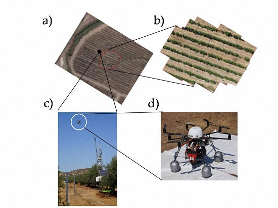
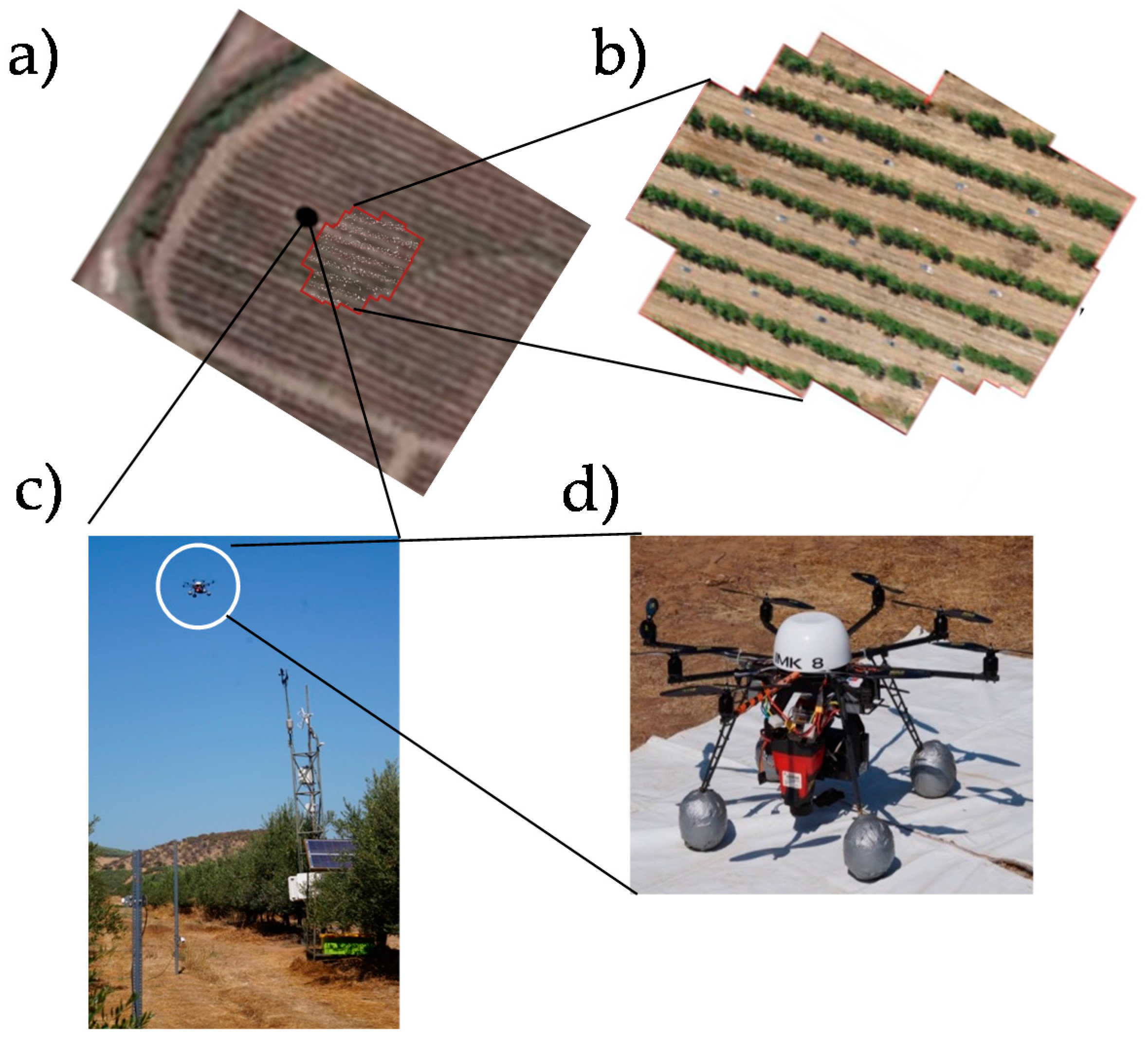
2.1. Study Site Description
2.2. Measurements of Energy Balance and Climatic Data
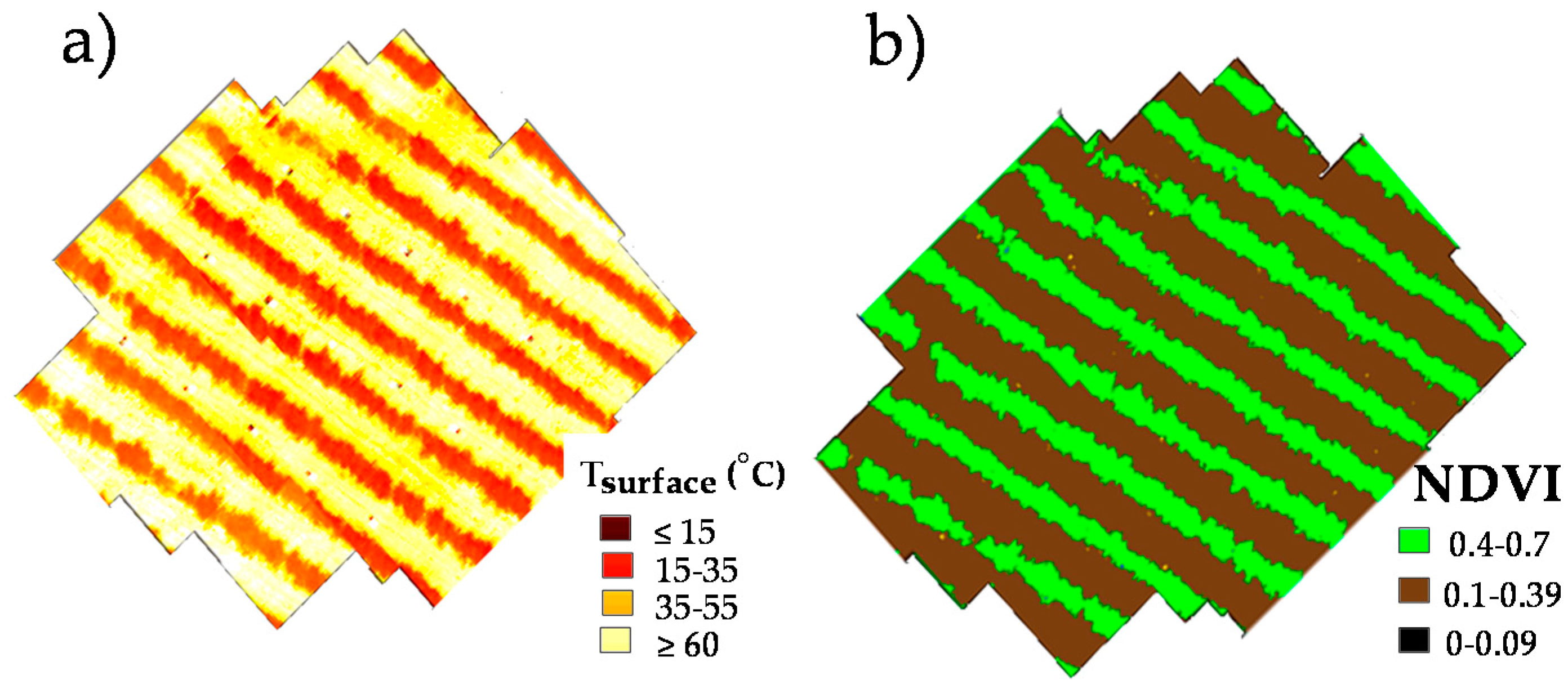
2.3. Thermal and Multispectral Images Acquisition and Processing
2.4. RSEB Algorithm Adapted for a Helicopter-Based UAV
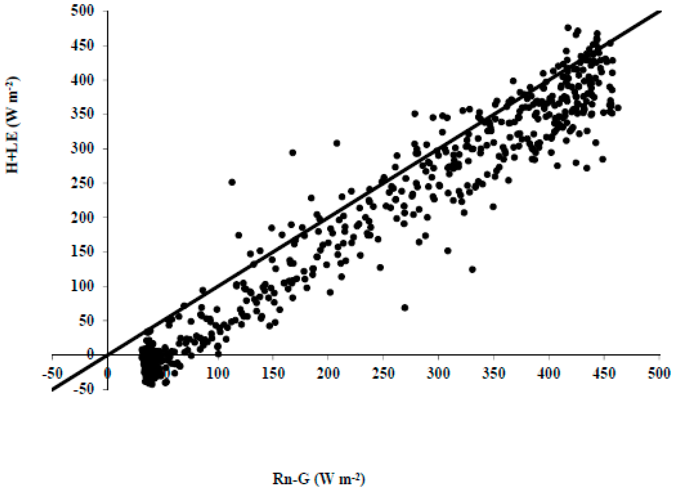
2.5. Statistical Analysis
3. Results
4. Discussions
5. Conclusions
Acknowledgments
Author Contributions
Conflicts of Interest
Appendix A. Expressions to Estimate the Aerodynamic Resistances in the RSEB Algorithm

| Symbol | Name | Value | |
|---|---|---|---|
| n | eddy diffusivity decay coefficient | 2.5 | obtained from [47] |
| x | reference height | 5.5 m | Measured |
| h | height of the canopy | 3.2 m | Measured |
| d | displacement height (0.63 × h) | 2.02 m | obtained from [47] |
| zOM | roughness length of crop (0.05 × h) | 0.16 m | obtained from [47] |
| z´o | roughness length of the bare soil (0.1 × zo) | 0.016 m | obtained from [47] |
| k | Von Karman’s constant | 0.41 | obtained from [47] |
| mean boundary layer resistance | 25 s m−1 |
References
- López-Olivari, R.; Ortega-Farías, S.; Poblete-Echeverría, C. Partitionning of net radiation and evapotranspiration over a superintensive drip-irrigated olive orchard. Irrig. Sci. 2016, 1, 17–31. [Google Scholar] [CrossRef]
- Intergovernmental Panel on Climate Change (IPCC). The Fifth Assessment Report (AR5); World Meteorological Organization (WMO): Geneva, Switzerland; United Nations Environment Programme (UNEP): Nairobi, Kenya, 2013. [Google Scholar]
- Fereres, E.; Soriano, M.A. Deficit irrigation for reducing agricultural water use. J. Exp. Bot. 2007, 58, 147–159. [Google Scholar] [CrossRef] [PubMed]
- Ortega-Farias, S.; Irmak, S.; Cuenca, R.H. Special issue on evapotranspiration measurement and modeling. Irrig. Sci. 2009, 28, 1–3. [Google Scholar] [CrossRef]
- Allen, R.G.; Pereira, L.S.; Raes, D.; Smith, M. Crop Evapotranspiration. Guidelines for Computing Crop Water Requirements; FAO Irrigation and Drainage Paper No. 56; Food and Agriculture Organization of the United Nations: Rome, Italy, 1998. [Google Scholar]
- Ortega-Farías, S.; Cuenca, R.H.; English, M. Hourly grass evapotranspiration in modified maritime environment. J. Irrig. Drain. Syst. 1995, 6, 369–373. [Google Scholar] [CrossRef]
- Alegre, S.; Marsal, J.; Mata, M.; Arbones, A.; Girona, J.; Tovar, M. Regulated deficit irrigation in olive trees (Olea europaea L. cv. ‘Arberquina’) for oil production. Acta Hortic. 2002, 586, 259–262. [Google Scholar] [CrossRef]
- Flores, F.; Ortega-Farías, S. Effect of Three Levels of Water Application on Oil Yield and Quality for an Olive (‘Picual’) Orchard. Acta Hortic. (ISHS) 2011, 889, 317–322. [Google Scholar] [CrossRef]
- Patumi, M.; D’Andria, R.; Marsilio, V.; Fontanazza, G.; Morelli, G.; Lanza, B. Olive and olive oil quality after intensive monocone olive growing (Olea europaea L., cv. Kalamata) in different irrigation regimes. Food Chem. 2002, 77, 27–34. [Google Scholar] [CrossRef]
- Tognetti, R.; d’Andria, R.; Morelli, G.; Alvino, A. The effect of deficit irrigation on seasonal variations of plant water use in Olea europaea L. Plant Soil 2005, 273, 139. [Google Scholar] [CrossRef]
- Cohen, Y.; Alchanatis, V.; Meron, M.; Saranga, S.; Tsipris, J. Estimation of leaf water potential by thermal imagery and spatial analysis. J. Exp. Bot. 2005, 56, 1843–1852. [Google Scholar] [CrossRef] [PubMed]
- Ortega-Farias, S.; Rigetti, T.; Acevedo, C.; Matus, F.; Moreno, Y. Irrigation-management decision system (IMDS) for vineyards (Region VI and VII of Chile). Integrated Soil Water Management for Orchard Development. FAO Land Water Bull. 2005, 10, 59–64. [Google Scholar]
- Carrasco-Benavides, M.; Ortega-Farías, S.; Lagos, L.O.; Kleissl, J.; Morales, L.; Poblete-Echeverría, C.; Allen, R.G. Crop coefficients and actual evapotranspiration for a drip-irrigated Merlot vineyard using multispectral satellite images. Irrig. Sci. 2012, 30, 537–553. [Google Scholar] [CrossRef]
- Carrasco-Benavides, M.; Ortega-Farías, S.; Lagos, L.O.; Kleissl, J.; Morales-Salinas, L.; Kilic, A. Parameterization of the Satellite-Based Model (METRIC) for the estimation of instantaneous surface energy balance components over a drip-irrigated vineyard. Remote Sens. 2014, 6, 11342–11371. [Google Scholar] [CrossRef]
- Samani, Z.; Bawazir, A.S.; Bleiweiss, M.; Skaggs, R.; Longworth, J.; Tran, V.D.; Pinon, A. Using remote sensing to evaluate the spatial variability of evapotranspiration and crop coefficient in the lower Rio Grande Valley, New Mexico. Irrig. Sci. 2009, 1, 93–100. [Google Scholar] [CrossRef]
- Allen, R.G.; Tasumi, M.; Morse, A.; Trezza, R.; Wright, J.L.; Bastiaanssen, W.; Kramber, W.; Lorite, I.; Robison, C.W. Satellite-based energy balance for mapping evapotranspiration with internalized calibration (METRIC) applications. J. Irrig. Drain. Eng. ASCE 2007, 4, 395–406. [Google Scholar] [CrossRef]
- Bastiaanssen, W.G.M.; Menenti, M.; Feddes, R.A.; Holtslag, A.A.M. A remote sensing surface energy balance algorithm for land (SEBAL)—1. Formulation. J. Hydrol. 1998, 1–4, 198–212. [Google Scholar] [CrossRef]
- Bastiaanssen, W.G.; Noordman, J.M.; Pelgrum, H.; Davids, G.; Thoreson, B.P.; Allen, R.G. SEBAL model with remotely sensed data to improve water-resources management under actual field conditions. J. Irrig. Drain. Eng. ASCE 2005, 1, 85–93. [Google Scholar] [CrossRef]
- Bastiaanssen, W.G.M. SEBAL-based sensible and latent heat fluxes in the irrigated Gediz Basin, Turkey. J. Hydrol. 2000, 229, 87–100. [Google Scholar] [CrossRef]
- Tasumi, M.; Allen, R.G.; Trezza, R.; Wright, J.L. Satellite-Based energy balance to assess within-population variance of crop coefficient curves. J. Irrig. Drain. Eng. ASCE 2005, 1, 94–109. [Google Scholar] [CrossRef]
- Tasumi, M.; Allen, R.G.; Trezza, R. At-surface reflectance and albedo from satellite for operational calculation of land surface energy balance. J. Hydrol. Eng. 2008, 2, 51–63. [Google Scholar] [CrossRef]
- Teixeira, A.; Bastiaanssen, W.G.M.; Ahmad, M.D.; Bos, M.G. Reviewing SEBAL input parameters for assessing evapotranspiration and water productivity for the Low-Middle Sao Francisco River basin, Brazil Part A: Calibration and validation. Agric. For. Meteorol. 2009, 3–4, 462–476. [Google Scholar] [CrossRef] [Green Version]
- Allen, R.; Irmak, A.; Trezza, R.; Hendrickx, J.M.H.; Bastiaanssen, W.; Kjaersgaard, J. Satellite-based ET estimation in agriculture using SEBAL and METRIC. Hydrol. Process. 2011, 26, 4011–4027. [Google Scholar] [CrossRef]
- Gowda, P.H.; Chávez, J.L.; Colaizzi, P.D.; Evett, S.R.; Howell, T.A.; Tolk, J.A. Remote sensing based energy balance algorithms for mapping ET: Current status and future challenges. Trans. ASABE 2007, 5, 1639–1644. [Google Scholar] [CrossRef]
- Gowda, P.H.; Chávez, J.L.; Colaizzi, P.D.; Evett, S.R.; Howell, T.A.; Tolk, J.A. ET mapping for agricultural water management: Present status and challenges. Irrig. Sci. 2008, 26, 223–237. [Google Scholar] [CrossRef]
- Elarab, M.; Ticlavilcab, A.; Torres-Ruab, A.; Maslovac, I.; McKeea, M. Estimating chlorophyll with thermal and broadband multispectralhigh resolution imagery from an unmanned aerial system using relevance vector machines for precision agriculture. Int. J. Appl. Earth Obs. Geoinf. 2015, 43, 32–42. [Google Scholar] [CrossRef]
- Liaghat, S.; Balasundram, S.K. A review: The role of remote sensing in precision agriculture. Am. J. Agric. Biol. Sci. 2010, 5, 50–55. [Google Scholar] [CrossRef]
- Berni, J.A.J.; Zarco-Tejada, P.J.; Suarez, L.; Fereres, E. Thermal and narrow-band multispectral remote rensing for vegetation monitoring from an unmanned aerial vehicle. IEEE Trans. Geosci. Remote Sens. 2009, 47, 722–738. [Google Scholar] [CrossRef]
- Berni, J.A.J.; Zarco-Tejada, P.J.; Sepulcre-Cantó, G.; Fereres, E.; Villalobos, F. Mapping canopy conductance and CWSI in olive orchards using high resolution thermal remote sensing imagery. Remote Sens. Environ. 2009, 113, 2380–2388. [Google Scholar] [CrossRef]
- Matese, A.; Toscano, P.; Filippo, S.; Gennaro, D.; Genesio, L.; Vaccari, F.P.; Primicerio, J.; Belli, C.; Zaldei, A.; Bianconi, R.; et al. Intercomparison of UAV, aircraft and satellite remote sensing platforms for precision viticulture. Remote Sens. 2015, 7, 2971–2990. [Google Scholar] [CrossRef]
- Ortega-Farías, S.; López-Olivari, R. Validation of a two-layer model to estimate latent heat flux and evapotranspiration over a drip-irrigated olive orchard. Trans. ASABE 2012, 4, 1169–1178. [Google Scholar] [CrossRef]
- Webb, E.K.; Pearman, G.I.; Leuning, R. Correction of flux measurements for density effects due to heat and water vapour transfer. Q. J. R. Meteorol. Soc. 1980, 106, 85–100. [Google Scholar] [CrossRef]
- Schotanus, P.; Nieuwstadt, F.T.M.; de Bruin, H.A.R. Temperature measurement with a sonic anemometer and its application to heat and moisture fluxes. Bound. Layer Meteorol. 1983, 26, 81–93. [Google Scholar] [CrossRef]
- Wilczak, J.M.; Oncley, S.P.; Stage, S.A. Sonic anemometer tilt correction algorithms. Bound. Layer Meteorol. 2001, 99, 127–150. [Google Scholar] [CrossRef]
- Ortega-Farias, S.; Poblete-Echeverría, C.; Brisson, N. Parameterization of a two layer model for estimating vineyard evapotranspiration using meteorological measurements. Agric. For. Meteorol. 2010, 150, 276–286. [Google Scholar] [CrossRef]
- Er-Raki, S.; Chehbouni, A.; Hoedjes, J.C.B.; Ezzahar, J.; Duchemin, B.; Jacob, F. Improvement of FAO-56 method for olive orchards through sequential assimilation of thermal infrared-based estimates of ET. Agric. Water Manag. 2008, 95, 309–321. [Google Scholar] [CrossRef]
- Martínez-Cob, A.; Faci, J.M. Evapotranspiration of an hedge-pruned olive orchard in semiarid area of NE Spain. Agric. Water Manag. 2010, 97, 410–418. [Google Scholar] [CrossRef] [Green Version]
- Twine, T.E.; Kustas, W.P.; Norman, J.M.; Cook, D.R.; Houser, P.R.; Meyers, T.P.; Prueger, J.H.; Starks, P.J.; Wesely, M.L. Correcting eddy covariance flux underestimates over a grassland. Agric. For. Meteorol. 2000, 103, 279–300. [Google Scholar] [CrossRef]
- Goward, S.N.; Markham, B.; Dye, D.G.; Dulaney, W.; Yang, J.L. Normalized difference vegetation index measurements from the advanced very high-resolution radiometer. Remote Sens. Environ. 1991, 35, 257–277. [Google Scholar] [CrossRef]
- Rouse, J.W.; Haas, R.H.; Schell, J.A.; Deering, D.W. Monitoring vegetation systems in the Great Plains with ERTS. In Third ERTS Symposium; Freden, S.C., Becker, M.A., Eds.; NASA Goddard Space Flight Center: Greenbelt, MD, USA, 1973; pp. 309–317. [Google Scholar]
- Zarco-Tejada, P.J.; Gonzalez-Dugo, V.; Berni, J.A.J. Fluorescence, temperature and narrowband indices acquired from a UAV platform for water stress detection using a micro-hyperspectral imager and a thermal camera. Remote Sens. Environ. 2012, 117, 322–337. [Google Scholar] [CrossRef]
- Corcóles, J.I.; Jose, F.; Ortega, J.F.; Hernández, D.; Moreno, M.A. Estimation of leaf area index in onion (Allium cepa L.) using an unmanned aerial vehicle. Biosyst. Eng. 2013, 115, 31–42. [Google Scholar] [CrossRef]
- Sanchez, J.M.; Lopez-Urrea, R.; Rubio, E.; Caselles, V. Determining water use of sorghum from two-source energy balance and radiometric temperatures. Hydrol. Earth Syst. Sci. 2011, 15, 3061–3070. [Google Scholar] [CrossRef]
- Sánchez, J.M.; López-Urreab, R.; Rubioc, E.; González-Piquerasd, J.; Caselles, V. Assessing crop coefficients of sunflower and canola using two-source energy balance and thermal radiometry. Agric. Water Manag. 2014, 137, 23–29. [Google Scholar] [CrossRef]
- Kustas, W.P.; Alfieri, J.G.; Anderson, M.C.; Colaizzi, P.D.; Prueger, J.H.; Evett, S.R.; Neale, C.; French, A.; Hipps, L.E.; Chávez, J.L.; et al. Evaluating the two-source energy balance model using local thermal and surface flux observations in a strongly advective irrigated agricultural area. Adv. Water Resour. 2012, 50, 120–133. [Google Scholar] [CrossRef]
- Poblete-Echeverría, C.; Ortega-Farias, S. Parameterization of surface energy balance components over a drip-irrigated Merlot vineyard using reflectance and meteorological data. Irrig. Sci. 2012, 30, 485–497. [Google Scholar]
- Long, D.; Singh, V.P. A modified surface energy balance algorithm for land (M-SEBAL) based on a trapezoidal framework. Water Resour. Res. 2012, 48. [Google Scholar] [CrossRef]
- Shuttleworth, W.J.; Wallace, J.S. Evaporation from sparse crops-an energy combination theory. Q. J. R. Met. Soc. 1985, 111, 839–855. [Google Scholar] [CrossRef]
- López-Olivari, R.; Ortega-Farías, S.; Morales, L.; Valdés, H. Evaluation of three semi-empirical approaches to estimate the net radiation over a drip-irrigated olive orchard. Chil. J. Agric. Res. 2015, 75, 341–349. [Google Scholar] [CrossRef]
- Gonzalez-Dugo, V.; Zarco-Tejada, P.; Berni, J.A.J.; Suárez, L.; Goldhamer, D.; Fereres, E. Almond tree canopy temperature reveals intra-crown variability that is water stress-dependent. Agric. For. Meteorol. 2012, 154–155, 156–165. [Google Scholar] [CrossRef]
- Willmott, C.J. On the validation of models. Phys. Geogr. 1981, 2, 184–194. [Google Scholar]
- Mayer, D.G.; Butler, D.G. Statistical validation. Ecol. Model. 1993, 1–2, 21–31. [Google Scholar] [CrossRef]
- Fernandes-Silva, A.A.; Ferreira, T.C.; Correia, C.M.; Malheiro, A.C.; Villalobos, F.J. Influence of different irrigation regimes on crop yield and water use efficiency of olive. Plant Soil 2010, 333, 35–47. [Google Scholar] [CrossRef]
- Ezzahar, J.; Chehbouni, A.; Hoedjes, J.C.B.; Er-raki, S.; Chehbouni, A.H.; Bonnefond, J.M.; De Bruin, H.A.R. The use of the scintillation technique for estimating and monitoring water consumption of olive orchards in a semi-arid region. Agric. Water Manag. 2007, 89, 173–184. [Google Scholar] [CrossRef] [Green Version]
- Er-Raki, S.; Chehbouni, A.; Boulet, G.; Williams, D.G. Using the dual approach of FAO56 for partitioning ET into soil and plant components for olive orchards in a semiarid region. Agric. Water Manag. 2010, 97, 1769–1778. [Google Scholar] [CrossRef] [Green Version]
- Villalobos, F.J.; Orgaz, F.; Testi, L.; Federes, E. Measurement and modeling of evapotranspiration of olive (Olea europaea L.) orchards. Eur. J. Agron. 2000, 13, 155–163. [Google Scholar] [CrossRef]
- Testi, L.; Orgaz, F.; Villalobos, F.J. Variations in bulk canopy conductance of an irrigated olive (Olea europaea L.) orchard. Environ. Exp. Bot. 2006, 55, 15–28. [Google Scholar] [CrossRef]
- Lee, X.; Black, T.A. Atmospheric turbulence within and above a douglas-fir stand. Part II. Eddy fluxes of sensible heat and water vapour. Bound. Layer Meteorol. 1993, 64, 369–389. [Google Scholar] [CrossRef]
- Wilson, K.; Goldstein, A.; Falge, E.; Aubinet, M.; Baldocchi, D.; Berbigier, P.; Bernhofer, C.; Ceulemans, R.; Dolman, H.; Field, C.; et al. Energy balance closure at FLUXNET sites. Agric. For. Meteorol. 2002, 113, 223–243. [Google Scholar] [CrossRef]
- Leuning, R.; van Gorsel, E.; Massman, W.J.; Isaac, P.R. Reflections on the surface energy imbalance problem. Agric. For. Meteorol. 2012, 156, 65–74. [Google Scholar] [CrossRef]
- Williams, D.G.; Cable, W.; Hultine, K.; Hoedjes, J.C.B.; Yepez, E.A.; Simonneaux, V.; Er-Raki, S.; Boulet, G.; de Bruin, H.A.R.; Chehbouni, A.; et al. Evapotranspiration components determined by stable isotope, sap flow and eddy covariance techniques. Agric. For. Meteorol. 2004, 125, 241–258. [Google Scholar] [CrossRef]
- Testi, L.; Villalobos, F.J.; Orgaz, F. Evapotranspiration of a young irrigated olive orchard in southern Spain. Agric. For. Meteorol. 2004, 121, 1–18. [Google Scholar] [CrossRef]
- Foken, T. The energy balance closure problem: An overview. Ecol. Appl. 2008, 18, 1351–1367. [Google Scholar] [CrossRef] [PubMed]
- Chávez, J.; Gowda, P.; Howell, T.; Neale, C.; Copeland, K. Estimating hourly crop ET using a two-source energy balance model and multispectral airborne imagery. Irrig. Sci. 2009, 28, 79–91. [Google Scholar] [CrossRef]
- Jusoff, K. Evaluation of spatial variability of soil in an oil palm plantation. In Proceedings of the ISCO 2004—13th International Soil Conservation Organization Conference, Brisbane, Australia, 4–8 July 2004.
- Liu, S.; Lu, L.; Mao, D.; Jia, L. Evaluating parameterizations of aerodynamic resistance to heat transfer using field measurements. Hydrol. Earth Syst. Sci. 2007, 11, 769–783. [Google Scholar] [CrossRef]
- Ortega-Farias, S.; Aguilar, R.; De la Fuente, D.; Ortega-Salaza, S.; Fuentes, F. Evaluation of a model to estimate net radiation over a drip-irrigated olive orchard using Landsat satellite images. Acta Hortic. (ISHS) 2014, 1057, 309–314. [Google Scholar] [CrossRef]
- Shaomin, L.; Guang, H.; Li, L.; Defa, M. Estimation of regional evapotranspiration by TM/ETM+ data over heterogeneous surfaces. Am. Soc. Photogramm. Remote Sens. 2007, 73, 1169–1178. [Google Scholar]
- González-Dugo, M.P.; González-Piqueras, J.; Campos, I.; Andréu, A.; Balbontín, C.; Calera, A. Evapotranspiration monitoring in a vineyard using satellite-based thermal remote sensing. SPIE Proc. 2012, 8531, 272–288. [Google Scholar]
- Ortega-Farias, S.; Aguilar, R.; De la Fuente, D.; Ortega-Salaza, S.; Fuentes, F.; Poblete-Echeverría, C. Estimation of evapotranspiration for a drip-irrigated olive orchard using multispectral satellite images. In Proceedings of the USCID Fourth International Conference on Irrigation and Drainage, Using 21st Century Technology to Better Manage Irrigation Water Supplies, Phoenix, AZ, USA, 16–19 April 2013.
- Xia, T.; Kustas, W.P.; Anderson, M.C.; Alfieri, J.G.; Gao, F.; McKee, L.; Prueger, J.H.; Geli, H.; Neale, C.M.U.; Sanchez, L.; et al. Mapping evapotranspiration with high-resolution aircraft imagery over vineyards using one- and two-source modeling schemes. Hydrol. Earth Syst. Sci. 2016, 20, 1523–1545. [Google Scholar] [CrossRef]
- Homann, H.; Nieto, H.; Jensen, R.; Guzinski, R.; Zarco-Tejada, P.J.; Friborg, T. Estimating evaporation with thermal UAV data and two-source energy balance models. Hydrol. Earth Syst. Sci. 2016, 20, 697–713. [Google Scholar] [CrossRef]


| Flight Date | Flight Time * | Rsi | Ta | RH | u | VPD |
|---|---|---|---|---|---|---|
| (DOY) | (hh:mm) | (W m−2) | (°C) | (%) | (m s−1) | (kPa) |
| 58 | 12:46 | 901 | 24.7 | 37.3 | 1.1 | 1.2 |
| 59 | 12:08 | 892 | 22.9 | 38.4 | 1.5 | 1.1 |
| 62 | 12:09 | 856 | 20.9 | 54.2 | 1.9 | 1.3 |
| 64 | 12:05 | 833 | 22.8 | 50.0 | 1.5 | 1.4 |
| 65 | 11:56 | 876 | 22.4 | 38.5 | 1.5 | 1.0 |
| 66 | 12:08 | 857 | 23.1 | 39.4 | 2.7 | 1.1 |
| 69 | 12:08 | 879 | 23.1 | 28.4 | 2.1 | 0.8 |
| 73 | 12:38 | 839 | 21.1 | 50.8 | 1.8 | 1.3 |
| 74 | 12:49 | 834 | 22.3 | 46.5 | 1.4 | 1.3 |
| 80 | 12:40 | 801 | 18.1 | 40.8 | 1.0 | 0.9 |
| Mean | 857 (±31) | 22.1 (±1.8) | 42.4 (±7.8) | 1.6 (±0.5) | 1.1 (±0.2) |
| DOY | Cr | β | Rn/Rsi | LEB/Rn | HB/Rn | G/Rn |
|---|---|---|---|---|---|---|
| 58 | 0.88 | 3.08 | 0.67 | 0.18 | 0.56 | 0.25 |
| 59 | 0.87 | 3.87 | 0.67 | 0.15 | 0.59 | 0.25 |
| 62 | 0.90 | 3.57 | 0.67 | 0.16 | 0.59 | 0.25 |
| 64 | 0.81 | 2.61 | 0.65 | 0.21 | 0.55 | 0.24 |
| 65 | 0.86 | 2.61 | 0.67 | 0.21 | 0.54 | 0.25 |
| 66 | 0.85 | 2.62 | 0.67 | 0.21 | 0.54 | 0.25 |
| 69 | 0.87 | 4.11 | 0.66 | 0.15 | 0.60 | 0.25 |
| 73 | 0.81 | 2.77 | 0.66 | 0.20 | 0.55 | 0.25 |
| 74 | 0.86 | 2.88 | 0.66 | 0.19 | 0.56 | 0.25 |
| 80 | 0.88 | 3.30 | 0.67 | 0.18 | 0.58 | 0.24 |
| Average | 0.86 (±0.03) | 3.09 (±1.7) | 0.66 (±0.01) | 0.18 (±0.02) | 0.57 (±0.02) | 0.25 (±0.00) |
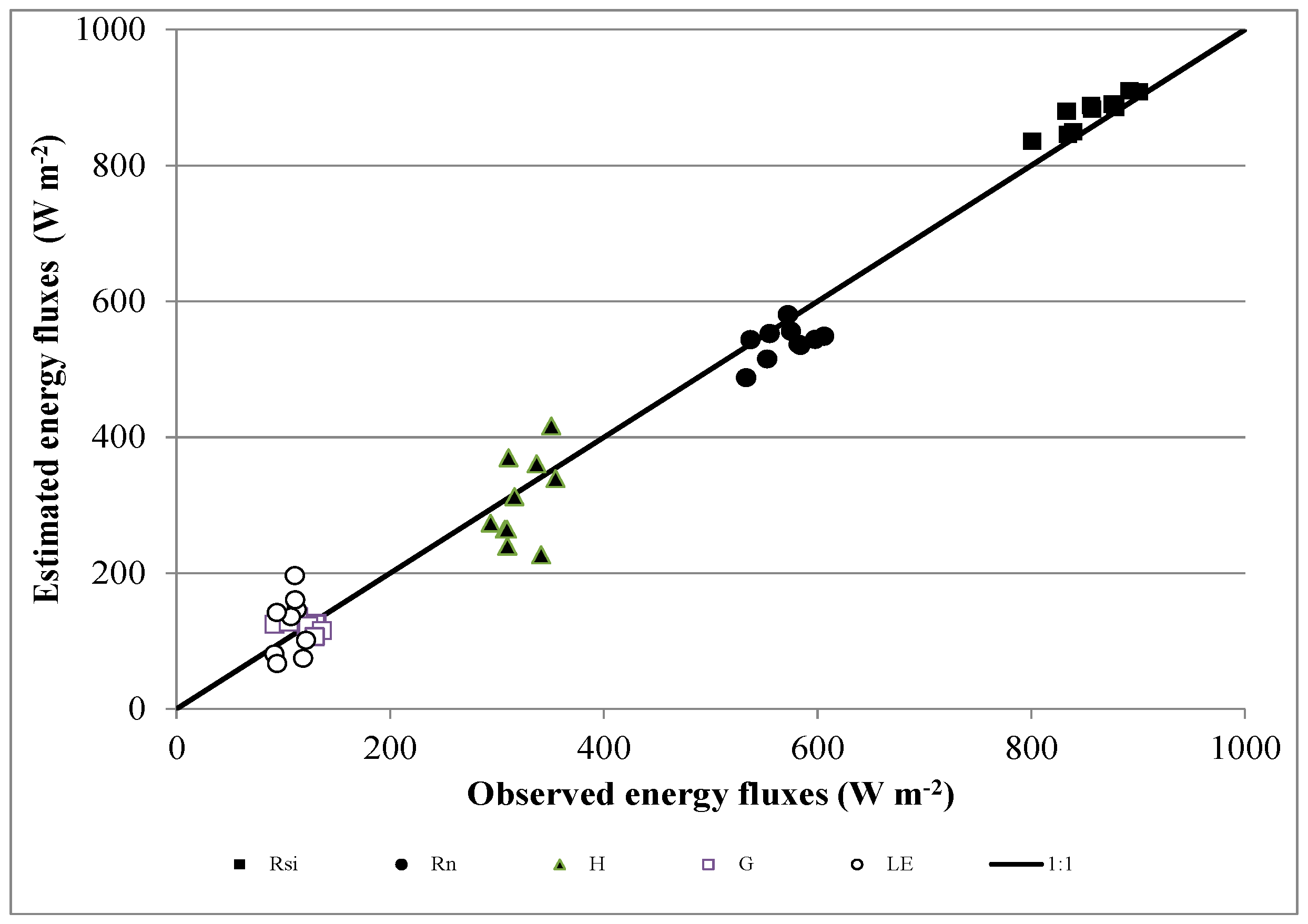
| Variable | RMSE (W m−2) | MAE (W m−2) | b | Ia | t-Test |
|---|---|---|---|---|---|
| Rsi | 24 | 21 | 1.02 | 0.92 | T |
| Rn | 38 | 33 | 0.95 | 0.88 | F |
| G | 19 | 16 | 1.02 | 0.66 | T |
| HB | 56 | 46 | 0.95 | 0.74 | F |
| LEB | 50 | 43 | 1.07 | 0.54 | F |
© 2016 by the authors; licensee MDPI, Basel, Switzerland. This article is an open access article distributed under the terms and conditions of the Creative Commons Attribution (CC-BY) license (http://creativecommons.org/licenses/by/4.0/).
Share and Cite
Ortega-Farías, S.; Ortega-Salazar, S.; Poblete, T.; Kilic, A.; Allen, R.; Poblete-Echeverría, C.; Ahumada-Orellana, L.; Zuñiga, M.; Sepúlveda, D. Estimation of Energy Balance Components over a Drip-Irrigated Olive Orchard Using Thermal and Multispectral Cameras Placed on a Helicopter-Based Unmanned Aerial Vehicle (UAV). Remote Sens. 2016, 8, 638. https://doi.org/10.3390/rs8080638
Ortega-Farías S, Ortega-Salazar S, Poblete T, Kilic A, Allen R, Poblete-Echeverría C, Ahumada-Orellana L, Zuñiga M, Sepúlveda D. Estimation of Energy Balance Components over a Drip-Irrigated Olive Orchard Using Thermal and Multispectral Cameras Placed on a Helicopter-Based Unmanned Aerial Vehicle (UAV). Remote Sensing. 2016; 8(8):638. https://doi.org/10.3390/rs8080638
Chicago/Turabian StyleOrtega-Farías, Samuel, Samuel Ortega-Salazar, Tomas Poblete, Ayse Kilic, Richard Allen, Carlos Poblete-Echeverría, Luis Ahumada-Orellana, Mauricio Zuñiga, and Daniel Sepúlveda. 2016. "Estimation of Energy Balance Components over a Drip-Irrigated Olive Orchard Using Thermal and Multispectral Cameras Placed on a Helicopter-Based Unmanned Aerial Vehicle (UAV)" Remote Sensing 8, no. 8: 638. https://doi.org/10.3390/rs8080638