Article

An Assessment of Pre- and Post Fire Near Surface Fuel Hazard in an Australian Dry Sclerophyll Forest Using Point Cloud Data Captured Using a Terrestrial Laser Scanner

1
School of Mathematical and Geospatial Sciences, RMIT University, Melbourne, VIC 3001, Australia
2
Bushfire and Natural Hazards Cooperative Research Centre, Melbourne, VIC 3002, Australia
*
Author to whom correspondence should be addressed.
Remote Sens. 2016, 8(8), 679; https://doi.org/10.3390/rs8080679
Submission received: 20 June 2016 / Revised: 5 August 2016 / Accepted: 16 August 2016 / Published: 20 August 2016

Abstract

:
Assessment of ecological and structrual changes induced by fire events is important for understanding the effects of fire, and planning future ecological and risk mitigation strategies. This study employs Terrestrial Laser Scanning (TLS) data captured at multiple points in time to monitor the changes in a dry sclerophyll forest induced by a prescribed burn. Point cloud data was collected for two plots; one plot undergoing a fire treatment, and the second plot remaining untreated, thereby acting as the control. Data was collected at three epochs (pre-fire, two weeks post fire and two years post fire). Coregistration of these multitemporal point clouds to within an acceptable tolerance was achieved through a two step process utilising permanent infield markers and manually extracted stem objects as reference targets. Metrics describing fuel height and fuel fragmentation were extracted from the point clouds for direct comparison with industry standard visual assessments. Measurements describing the change (or lack thereof) in the control plot indicate that the method of data capture and coregistration were achieved with the required accuracy to monitor fire induced change. Results from the fire affected plot show that immediately post fire 67% of area had been burnt with the average fuel height decreasing from 0.33 to 0.13 m. At two years post-fire the fuel remained signicantly lower (0.11 m) and more fragmented in comparison to pre-fire levels. Results in both the control and fire altered plot were comparable to synchronus onground visual assessment. The advantage of TLS over the visual assessment method is, however, demonstrated through the use of two physical and spatially quantifiable metrics to describe fuel change. These results highlight the capabilities of multitemporal TLS data for measuring and mapping changes in the three dimensional structure of vegetation. Metrics from point clouds can be derived to provide quantified estimates of surface and near-surface fuel loss and accumulation, and inform prescribed burn efficacy and burn severity reporting.

Graphical Abstract

1. Introduction

Prescribed burning is commonly practiced across many fire prone landscapes in order to mitigate the negative impacts of wildfire by reducing fuel hazard, and to promote positive ecological effects [1]. Many countries have policy and legislative requirements for achieving minimum prescribed burning targets (for example [2]). However, there remains an ongoing debate about the efficacy of such practices (for example [3]) largely driven by uncertainties by the lack of high-level quantitative data recorded for fuel and ecological changes, and the immediate effectiveness and longitudinal consequences of prescribed burning [4]. Indeed, the effects of fire can be quite variable between different ecosystems [5] and within ecosystems depending upon fire intensity, seasonality and past fire history. In addition, whilst prescribed burning plays a role in reducing the likelihood of severe wildfire and the associated risk to biological and economic values, prescribed burning for fuel reduction purposes can also negatively impact biodiversity values [6]. As such, repeatable, accurate and quantified post-fire vegetation monitoring can be considered a crucial factor informing current and future land management understandings and activities.
Current methods for assessing burn effects and post fire landscape evolution rely on in situ visual interpretation (see [7]) or interperation of aerial or satellite imagery [8]. Visual interpretation of fuel hazard and fire severity has been shown to be inconsistent between observers [9] and often do not provide quantified estimates of vegetation properties. While aerial and satellite imagery interpretation may not provide a full 3D description of the change and often suffers from high levels of occulusion when assessing changes in near ground vegetation due to an unburnt canopy [8].
Laser scanning technology has been shown to provide a highly accurate 3D representation of the natural landscape. Information describing forest fuel conditions has been captured from laser scanning systems deployed both on aircraft [10,11], as well as terrestrially [12,13,14]. Although capturing the properties of subcanopy vegetation is possible using airborne data, the ability to detect detailed information and change in these layers remains an ongoing challenge [15].
Terrestrial Laser Scanning (TLS) scanners operate insitu and as such produce a near complete description of the immediate area by generating high density point clouds (with point densities reaching up to multiple points per cm). This high density has been shown to allow information describing the properties of surface and near ground vegetation to be extracted. For example, Greaves et al. [16] and Olsoy et al. [17] demonstrated the utility of TLS in providing accurate measurement of near ground biomass in contrasting environments. Gupta et al. [18] demonstrated the sensitivities of TLS measurement to fire disturbances. These authors demonstrated that changes in TLS metrics derived from multi-temporal data capture can be attributed to actual on ground processes.
Several studies have also shown the potential in the use of TLS for mult-temporal analysis of near-ground vegetation in agricultural [19,20,21], desert [22], and artic [16] environments through the extraction of metrics such as plant height and volume. Sankey et al. [22], for example, showed that repeat TLS measurement can be used to monitor changes in the height of sparsely vegetated plots. These authors found that change in TLS height observation showed strong corellation (r2 = 0.8) to field measurements made using a total station.
The objective of this paper is to apply TLS technology and processing algorithms to detect and describe the longitudal changes induced by a prescribed burn. In addition, we present a strategy for the collection and analysis of multi-temporal TLS data captured before and at two stages (two weeks post-fire and two years post-fire) following a low intensity prescribed fire.

2. Materials and Methods
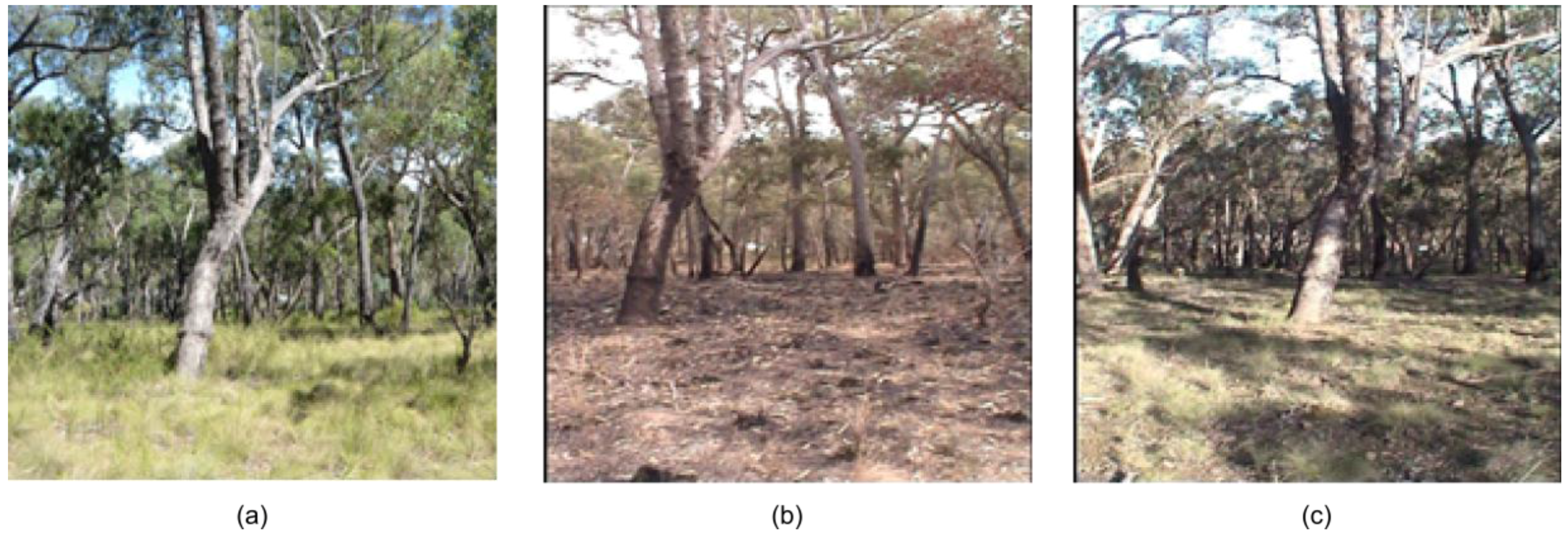
2.1. Study Area

This study was conducted in a dry sclerophyll forest in St. Andrews, approximately 45 km northeast of metropolitan Melbourne, Victoria, Australia. The canopy, dominated by eucalypt species, had a height of between 10 and 12 m and an approximate base height of between 5 and 7 m. Little to no mid-storey vegetation was present at the site. Near-surface and surface fuels, composed of grasses and woody debris, did not exceed 1 m in height across the study area (Figure 1).
A fuel reduction burn was undertaken in the area by land management agencies on 15 April 2012. Prior to the burn two 10-m radius circular plots were subjectively located within the proposed planned burn area. The plots were chosen to have similar topography and near-surface fuel composition and arrangement. A fire break was established surrounding Plot 1 prior to the burn. This plot acted as control and received no fire treatment. Plot 2 was fire treated as per prescription for the site. The fire temperature in this plot, recorded using temperature sensitive crayons and paints placed at ground level, reached 600 °C.

2.2. Field Data

Field observation and remotely sensed data were collected two weeks prior to the burn (pre-fire), two weeks following the burn (post-fire) and two years following the burn (recovery). Field observations at the pre-fire and recovery stages were collected in the form of fuel hazard assessment following Hines et al. [7] and Cawson et al. [23]. These guides required estimates of plot level percent cover and fuel height to be made for both the surface litter layer and near surface vegetation separately. Percent cover was recovered by making a visual estimate from the center of the plot. Percent area burnt was estimated post-fire using the same method. Fuel height was taken as the average height of 10 measurements randomly located using a ruler.

2.3. TLS Data

Each TLS survey was completed using the same Trimble CX scanner and utilising the same instrument set-up. Utilising the same scanner through multiple measurements epoch allowed for direct comparison of the derived information. This scanner emits visible red light pulses (660 nm) with a scan rate of 54,000 pulses per second. Each scan was set to capture the maximum available field-of-view, being 360° horizontally and 300° vertically, with a point spacing of 0.01 m at a distance of 10 m from the scanner. A single scan was captured from the center of each plot, with the scan completed in approximately 45 min. Single scan capture was preferred over multiple scans due to time constraints surrounding the burn scenario.

2.4. TLS Data Processing

The multi-temporal point clouds from each plot were coregistered in a two step procedure. The first step involved manually coordinating the center point of a permanent reference target (a stainless steel tag permanently fixed to a stem in the plot). Locating the reference targets, present as a patch of high intensity points. This allowed a 3D translation and rotation to be applied to each point cloud to achieve a coarse co-registration.
This coarse registration was refined in the second step which made use of the Iterative Closest Point (ICP) algorithm. The ICP algorithm was applied to point clouds in which all returns close to the surface and originating from leafy or fine vegetation had been manually removed, leaving only returns originating from tree stems. The manual process to achieve this stem only dataset was undertaken in CloudCompare software and involved first selecting points that occurred approximately between 0.8 and 2.5 m above ground level. This set of points was then refined by removing all points that did not obviously originate from a stem. The resultant point clouds provided 13 stem objects for Plot 1 and 11 stem objects for Plot 2. These stems were well distributed across the plot. Using these point clouds minimised the effect of scene evolution and wind differences between data captures. The point cloud of stem objects from post-fire was used as the model point cloud for which transformation parameters (3D translation and rotation) for the pre-fire and recovery point clouds were determined based on the ICP algorithm results. These transformations were then applied to all points captured at pre-fire and recovery.
A mask was then applied to remove points not originating from fuels connected to the surface (mid-layer and canopy levels). This mask was manually digitised for each plot in cloud compare, with the same mask applied to each multi-temporal point cloud. The effect of occlusion was seen to vary between epochs owing to differences in the arrangement of near-surface vegetation and small variations in the TLS scanner location. Subsequently a second mask was applied to avoid occlusion affecting the results. The mask was created following Gupta et al. [18]. In brief, a 2D α-shape (α = 0.1) was calculated for each near-surface point cloud of a plot. The intersection of these alpha shapes was then used to keep only points in areas where occlusion had not occurred during any of the surveys for that plot.

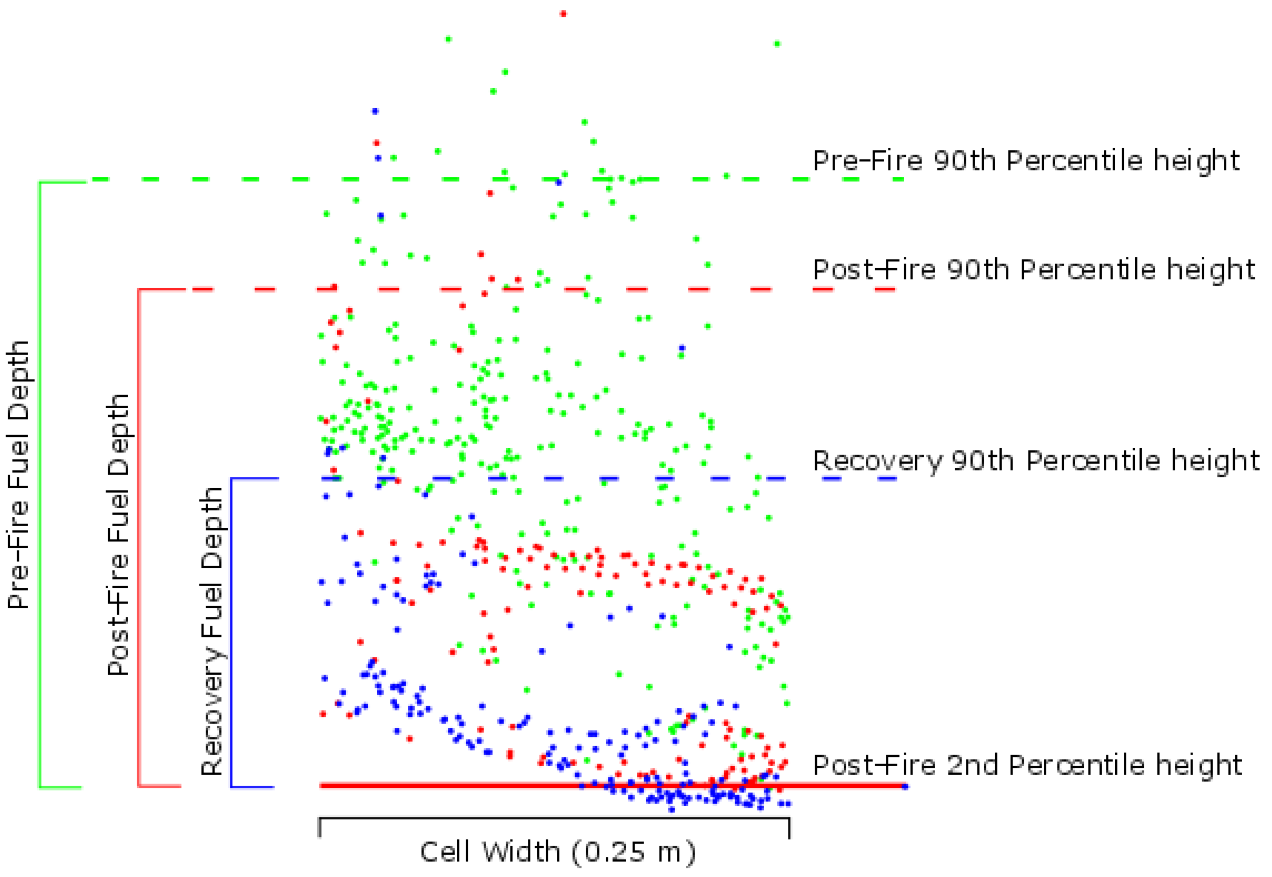
2.5. Fuel Hazard Assessment

We assess fuel hazard and its change through time using two metrics, fuel depth and horizontal connectivity utilising a 0.25 × 0.25 m grid. For each cell, fuel depth was calculated as the vertical distance between estimates of the terrain height and the dominant of the near-surface fuel height (Figure 2). Terrain height was held static across the three measurement stages and was calculated as the 2nd percentile of the point height distribution from the post-fire data. The post-fire height distribution was used to determine the minimum height as this point cloud contained the least amount of vegetation. The near-surface vegetation height was calculated, separately for each measurement stage, as the 90th percentile of the point height distribution. This method was prefered over calculating above ground height due to issues in accurately detecting ground points. Fuel depth was converted to a plot level estimate of fuel volume based on the assumption that the fuel in any cell was contiguous to ground level. As such, volume was calculated as the cell area (0.0625 m2) multiplied by fuel depth.
Fuel fragmentation was measured by creating a 2D fuel cover binary grid. A cell was marked as having fuel present when 50% of the points in a cell occurred at height greater than 0.05 m above the post-fire 2nd percentile. The 0.05-m threshold was determined by the average slope across both plots. Fuel fragmentation was assessed based on the properties of each unique patch within the plot, with number of patches, mean patch area and the mean nearest neighbour distance calculated. Where the mean nearest neighbour distance is defined as the average edge-to-edge distance (m) between a patch and its nearest neighbour in the landscape. For this process, an assumption was made that occluded cells have no fuel cover.

3. Results

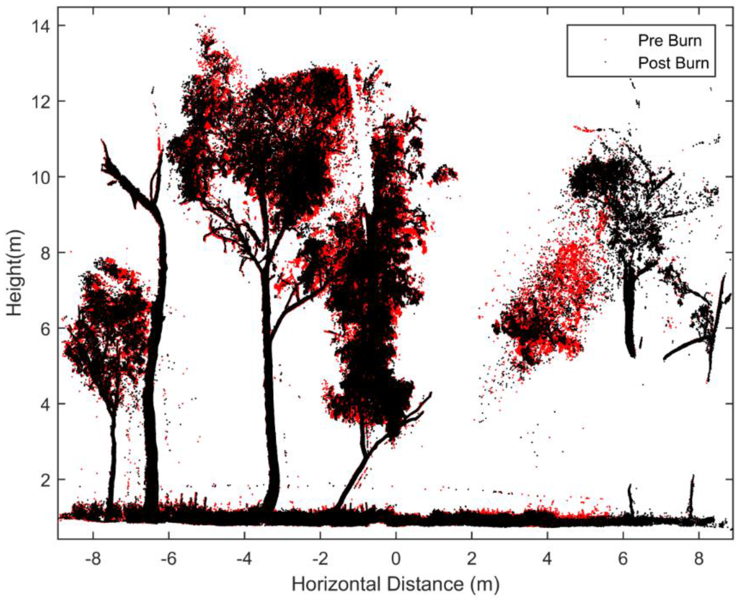
3.1. Point Cloud Properties

Visual inspection of the point clouds indicate that the two step co-registration approach has been successful in co-registering multi-temporal point clouds (Figure 3). The coregistraion process took less than one hour per plot. The translation and rotation parameters derived from the ICP algorithm were less than 3 cm and 0.5°, respectively. Visual examination of the resultant coregistation indicated remaining point cloud misalignment to be well within the magnitude of the ICP determined transformation. Given that further analysis utilised a 0.25-m resolution grid, this level of accuracy was considered acceptable. Variations in the landscape conditions due to fire disturbance, growth, senescene, human and animal disturbance, as well as differing wind conditions at the time of each scan, are likely to preclude a more accurate coregistration using this data.
For all point clouds, the point density within any one cell varied between 40,000 points per m2 close to the sensor and 500 points per m2 near the plot edge. Nineteen percent to 22% of the area of Plot 1 scan was occluded in each TLS scan, with the combined occlusion mask covering 27% of the plot. The majority of this occlusion was caused by three large stems at 4–7 m from the scanner position. The area of Plot 2 was between 13% and 15% occluded in the three scans with the combined occlusion mask covering 15% of the plot.

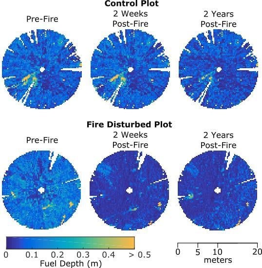
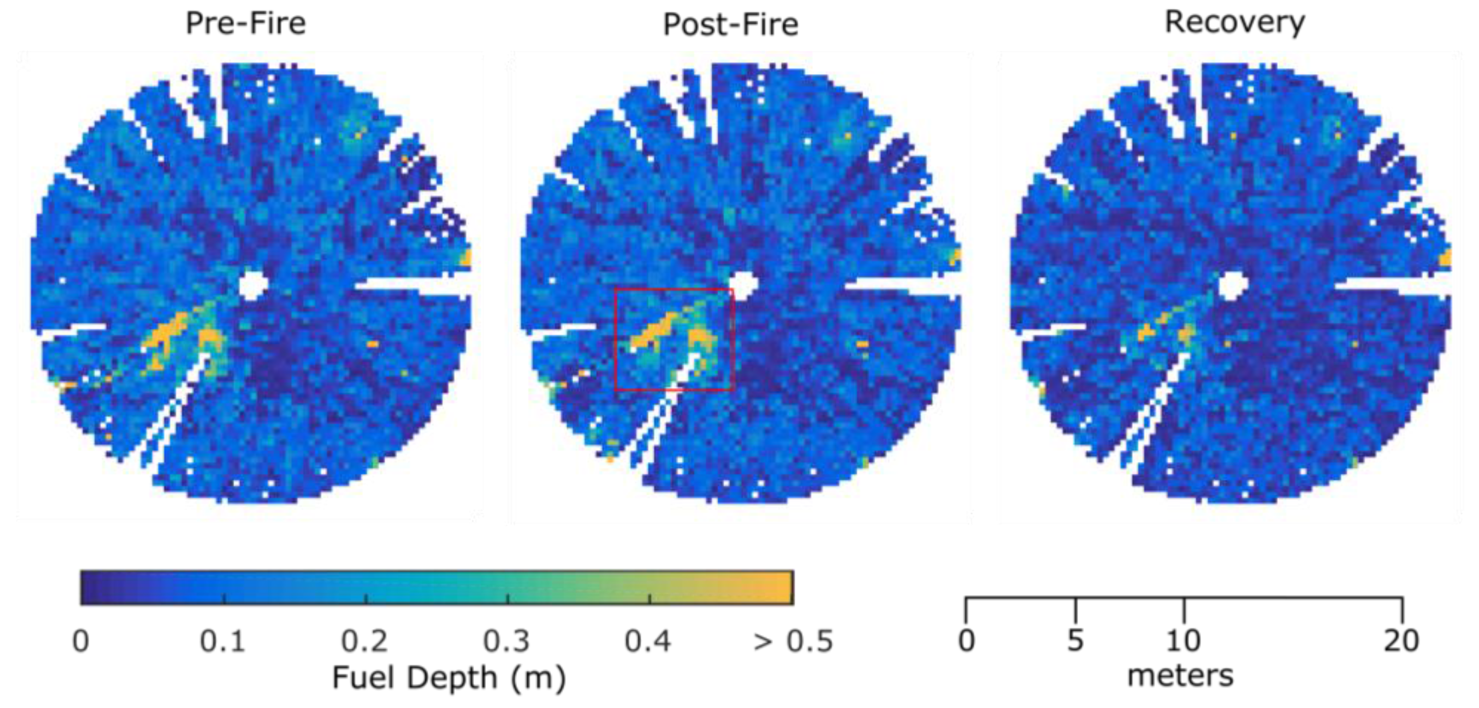
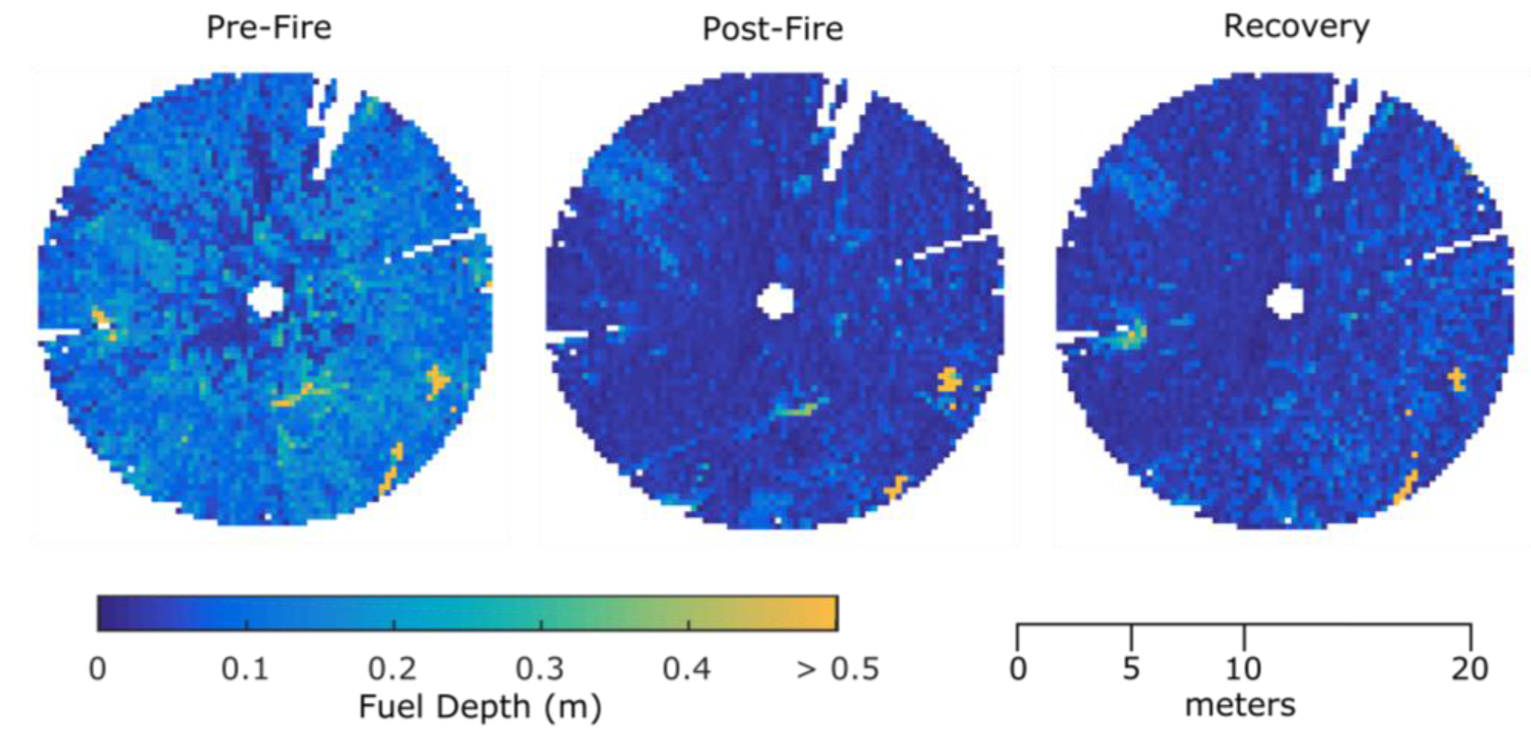
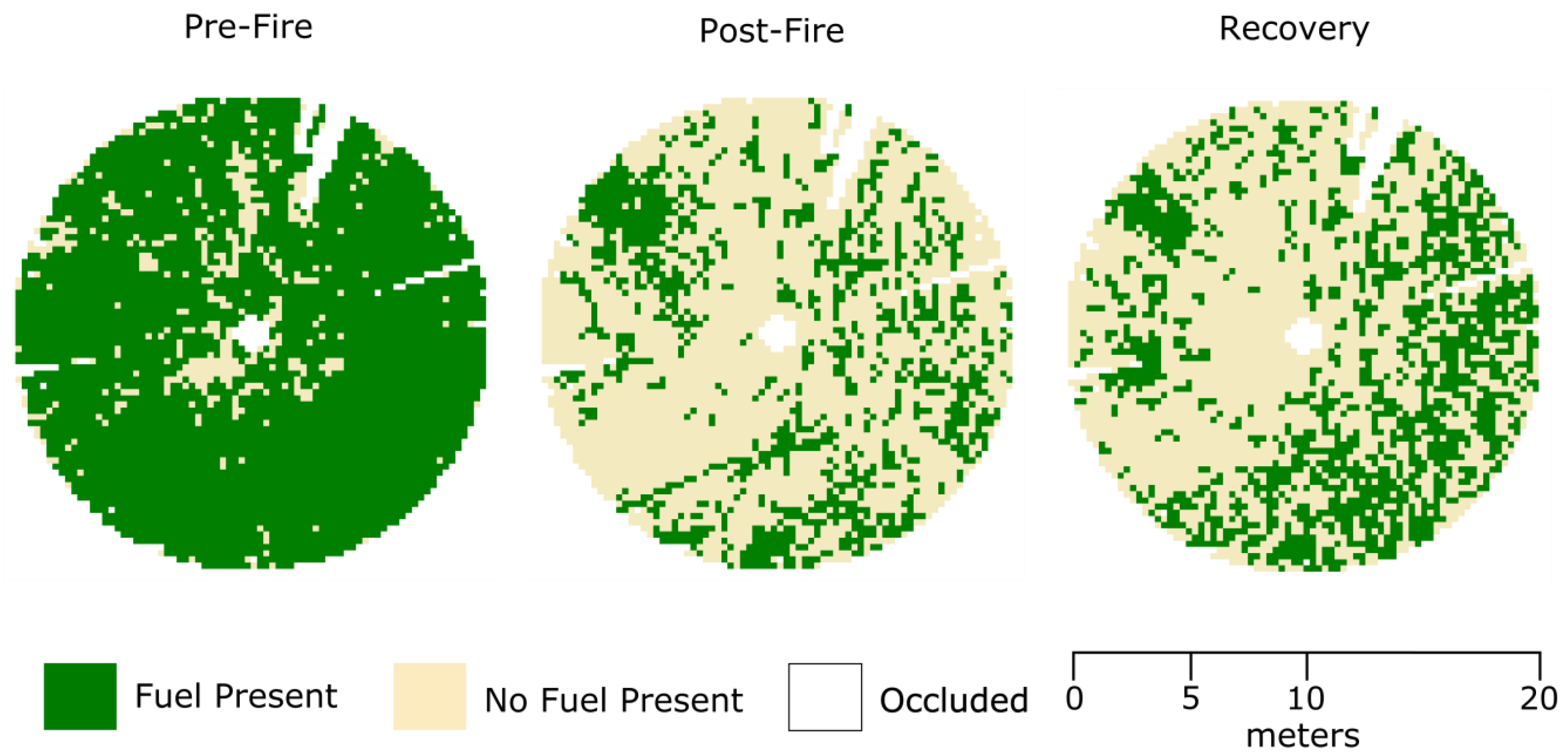
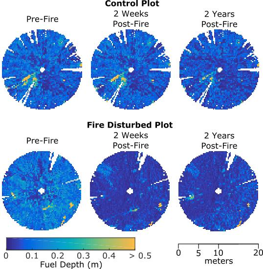
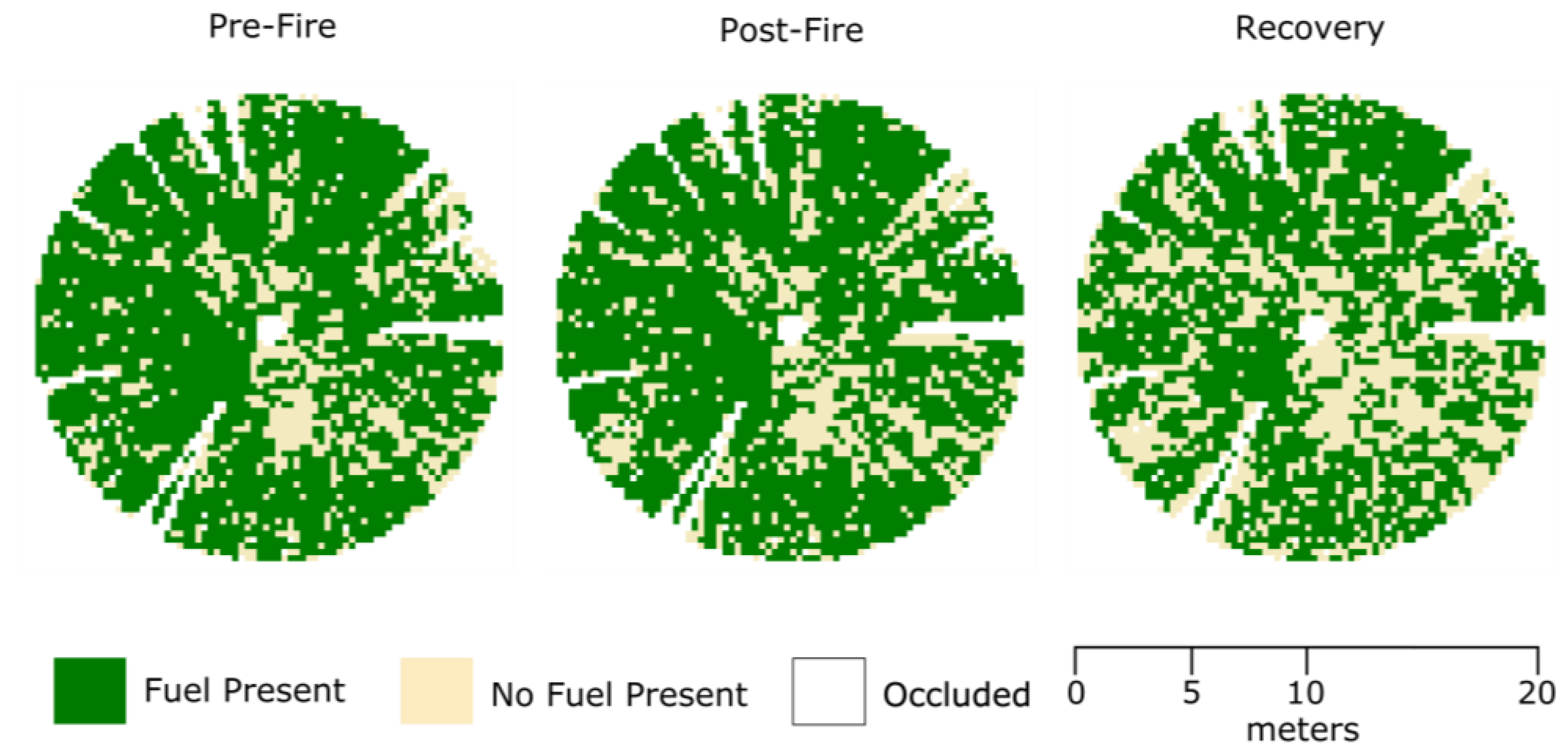
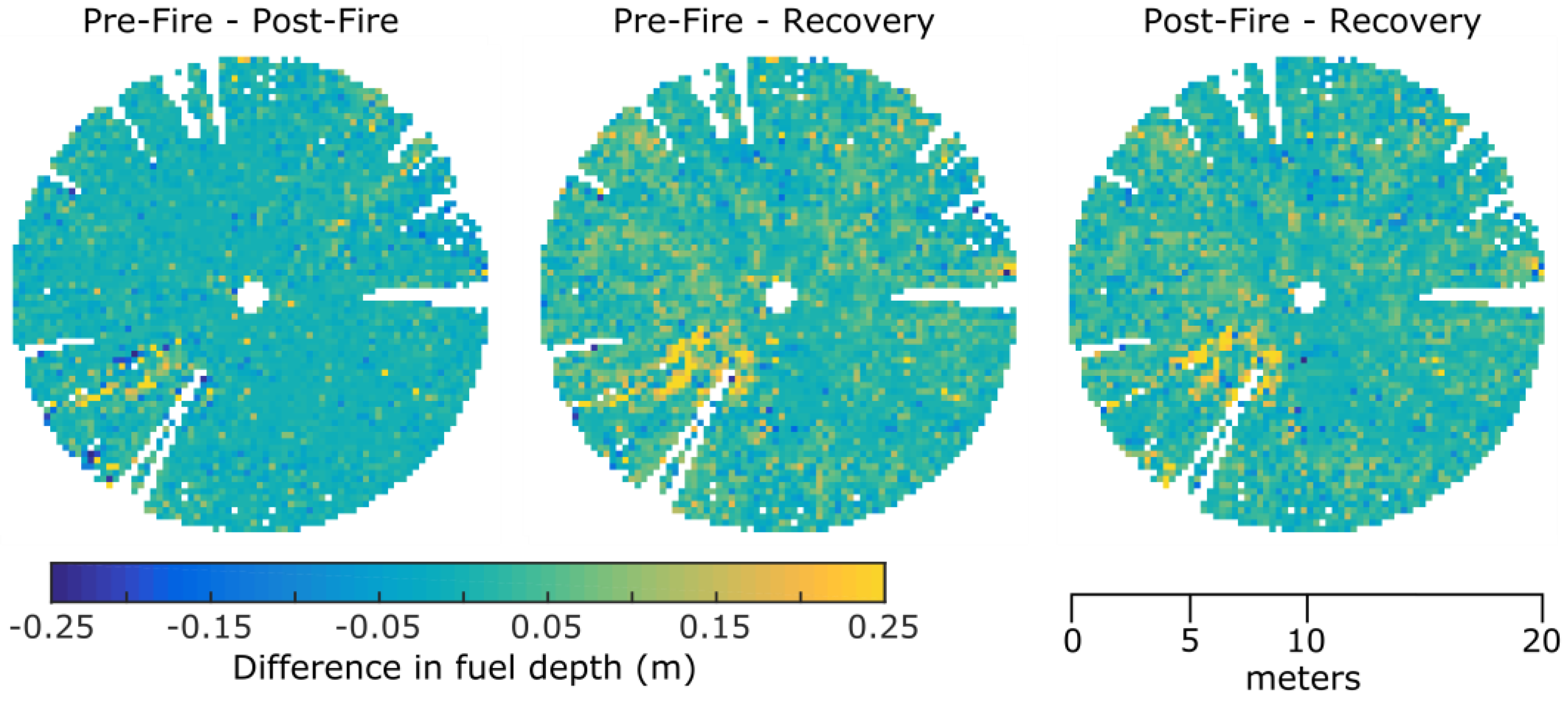
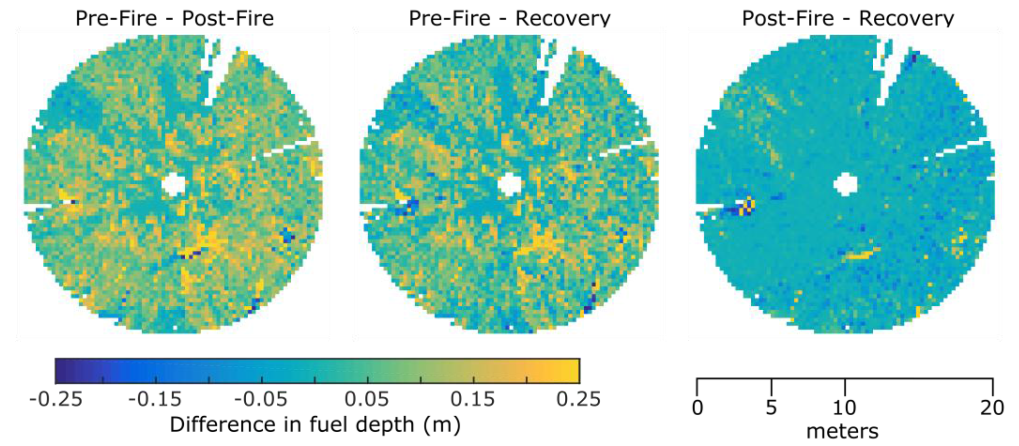
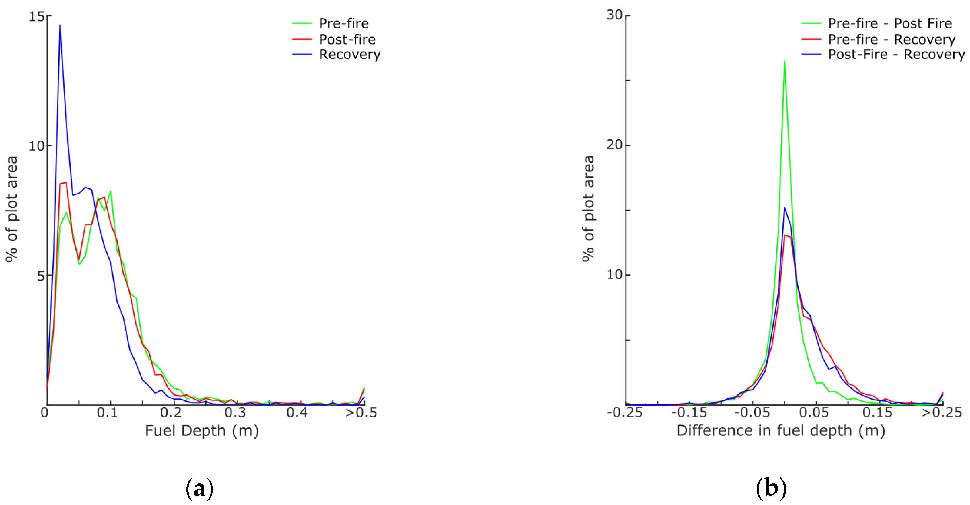
3.2. TLS Described Fuel Hazard Evolution

3.2.1. Pre-Fire Fuel Hazard

Analysis of the TLS metrics suggested that the pre-fire fuel hazard landscape was similar in both plots (Figure 4 and Figure 5). Plot 1 had a mean fuel depth of 0.21 ± 0.13 m, the maximum near surface fuel depth of 1.51 m occurred due to a recently fallen tree near the plot center. The estimated fuel volume in this plot was 56.05 m3. Plot 2 was observed to have higher fuel levels (estimated volume of 95.06 m3 and mean depth of 0.33 ± 0.19 m) and a maximum fuel depth of 1.43 m, occurring due to a small juvenile tree in the south-east region of the plot.
Pre-fire both plots presented similar contiguous horizontal fuel distribution and contained one large fuel patch covering the majority of the plot and three smaller patches (Figure 6 and Figure 7). The total area of these patches was 209 m2 (74% of plot area) and 254 m2 (90% of plot area) for Plots 1 and 2, respectively. Following Hines et al. [7], analysis of TLS data suggests both plots have similar fuel hazard, with levels of fuel cover representing an extreme fuel hazard score.

3.2.2. Post-Fire Fuel Hazard Reduction

As expected the post fire fuel hazard for Plot 1 presented very little change when observed two weeks post-fire. The mean fuel depth decreased slightly to 0.18 ± 0.12 m, resulting in an overall decrease in volume of 8 m3 (to 49.01 m2). The majority of the variation in fuel depth primarily occurred in the area of the fallen tree with maximum depth falling to 1.40 m2 (Figure 8). Fuel fragmentation increased slightly with 63% of the plot (204 m2) being covered by 7 patches. Similar to the conditions pre-fire, the fuel cover was comprised of a single large patch and three smaller patches.
In contrast to Plot 1, the TLS data indicated that the fuel hazard was significantly reduced in Plot 2. Fuel depth dropped by 0.20 ± 0.17 m on average (to a post fire mean depth of 0.13 ± 0.17 m) across the plot (Figure 9). Reducing plot level fuel volume to 38 m3. Notably the fuel depth was reduced by more than 0.05 m in 76% of cells. While only 13% of the cells showed an increase greater than 0.05 m. Visual analysis of the raw point cloud and fuel depth maps indicated increases in fuel depth, can be attributed to actual changes in the position of woody debris due to disturbance; small scale variations in occlusion causing fuel to be visible that was not in previous scans; and slight misregistration errors causing returns from high vegetation near cell edges to be attributed to different cells.
The TLS scan taken two weeks post fire indicated that the fuel fragmentation dramatically increased in Plot 2. The total fuel covered area decreased to 23% of the plot area (74 m2), with this fuel split between 95 small patches (mean area 0.78 ± 2.09 m2). The nearest neighbour metric indicated a mean minimum distance of 0.59 m. The mean area of fuel patches was significantly less than the mean area of non-fuel patches (six non-fuel patches with a mean area of 33 ± 88 m2) in this plot.

3.2.3 Post-Fire Vegetation Recovery

TLS metrics extracted from the Plot 1 point cloud indicated a decrease in overall fuel volume (37 m3) at the recovery measurement stage (two years post fire). This was largely driven by changes to the structure of the fuel at, and immediately surrounding, the fallen tree. Average change in fuel depth was –0.07 ± 0.11 m and –0.04 ± 0.10 m between Pre-Fire and Post-Fire estimates respectively (Figure 10). The fuel at Plot 1 remained as mostly one contiguous patch, however, the number of smaller fuel patches increased to 13 (mean area 13.09 ± 5.74 m2).
The TLS data indicates that the fuel levels in Plot 2 have not recovered to Pre-Fire levels at the Recovery stage. Average fuel depth (0.11 ± 0.14 m) was found to be shallower than at both the Pre-Fire and Post-Fire stages. In comparison to fuel depth at Pre-Fire estimates, 91% of the observed plot area had a decreased fuel depth of 5 cm or more. The mean decrease in depth (0.23 ± 17 m) was greater than the decrease in depth observed two weeks post fire. Compared to the Post-Fire fuel level estimates, the distribution of fuel depth remains similar (Figure 11). Nevertheless, variation in depth occurred across the plot with 15% of the area increasing and 27% decreasing in fuel depth by greater than 5 cm. The overall fuel volume of 30 m3 is slightly lower than that observed at the Post-Fire stage (38 m3).
Although fuel depth and volume had decreased since post-fire, the fuel connectivity appears to have begun to recover at the Recovery stage. The total fuel cover increased by 30% to 97 m2 split across 83 patches (mean area 1.17 ± 5.74 m2). Notably, this increase in fuel cover occurred mainly in the south east of the plot due to a 51.00 m2 contiguous patch of fuel. Although the fuel became more connected in this area, the mean minimum nearest neighbour distance (0.58 m) did not change significantly. This is due to an increase in fragmentation of the fuels in the north east of the plot.

3.3 Comparison to Field Observations

Interpretation of the field observations suggest similar changes to fuel hazard to those from the above analysis across Plots 1 and 2 (Table 1 and Table 2). Percent cover was estimated to be similar at the various pre-burn and post-fire stages in both Plots 1 and 2. Notably the change in cover between pre-fire and post-fire TLS estimates (67%) was similar to the estimates of burnt area (60%–70%). Field observations suggested that the fuel cover in Plot 2 had significantly increased by the recovery stage, primarily driven by an increase in litter to above pre-burn cover levels (an indicated increase of 10% to 20%). However, the magnitude of the increase in cover measured using the TLS data was significantly smaller (7%).
In contrast to the field estimates, the metrics derived from the TLS data did not distinguish between surface and near-surface fuels. Nevertheless, the estimates of fuel height appear to mostly agree. For instance, post-burn fuel height estimated at 0.13 m by TLS analysis was estimated to be 0.1 m to 0.2 m for both surface and near-surface vegetation, respectively.

4. Discussion

4.1. Multi-Temporal Monitoring of Vegetation and Fuel Hazard Changes Using TLS

Several approaches for measuring and monitoring the structural properties of vegetation using TLS have been outlined within the literature. These studies, which typically focus on measuring variations in tree form [24] or biomass [24,25,26] and the growth of agricultural crops [19,20,21], highlight the accuracy that can be achieved using TLS technology for these purposes. The objective of this study was, to apply similar methods to assess change induced by fire within Australian dry sclerophyll forests. As such, the methods used, while similar to these studies, have been adapted to suit both the environment and the agent of change.
Previous studies (such as [27]) have highlighted the importance of collecting multi-scan data in forests with high stem densities. However, in this study a single scan approach was used to collect TLS data. While a multi-scan approach would have likely allowed 100% of the plot to be assessed, this would have added further complexity to the processing chain. Given the low stem density present in the study area, the trade-off in processing effort for accuracy was not warranted. Results showed a suitably high percentage of the plot area to be observed at all times (73% in Plot 1 and 83% in Plot 2). This resulted in an accurate map showing fuel presence or absence, as well as an estimate of fuel volume in the observed area.
The presence of a fire disturbance in a forest setting precluded the use of permanent reference objects within the landscape to perform point cloud coregistration. As such, a similar approach to Liang et al. [24], Srinivasan et al. [25], and Hoffmeister et al. [19] was undertaken which utilised one fixed target and a fixed instrument set up location. The presence of fire resulted in movement of these targets between subsequent surveys and further refinement using the stem objects was undertaken. Although the results of this process were deemed acceptable, the accuracy of the coregistration using this method precluded a fine scale analysis. Subsequently this study utilised a 0.25-m grid to describe the fuel conditions. This resolution was deemed adequate to describe certain metrics such as fuel depth and fragmentation, however, variations in other important properties could not be quantified. For example, the relative accuracy between points within a TLS point cloud is very high and such data has the potential to allow feature-based descriptions of fuel properties such as fuel fineness and vertical compactness to be extracted. Comparison of these more detailed properties at multiple epochs would, however, required a higher accuracy coregistration to be achieved. However, for much post-fire reporting, plot-level information is sufficient.

4.2. Comparison to Current Fuel Assessment Methods

Visual assessment guidelines (such as [7]) outline a number of key metrics that are required to be observed in the field for assessing surface and near-surface fuel hazard. These include fuel height, % cover and % dead or alive. While an assessment of % dead or alive was not attempted, this study has demonstrated that TLS is capable of quantitatively assessing changes in fuel height and % cover. In addition, information about the spatial connectivity or fragmentation of the fuel can also be obtained providing further insight into the types of change incurred in the landscape. In comparison to visual assessments, where metrics are observered through a limited number of samples or ocularly [7], the approach taken here provides description of fuel hazard in the form of multi-temporal maps and height estimates which allow for a quantified and objective description of the fuel hazard environment, as well as a non-subject assessment for use in understanding its dynamics.
Visually assessed fuel height was achieved by attributing fuel height into 10-cm bins. Average fuel depth measured using TLS fell within, or close to these bins. It should be noted that this comparison does not provide a rigourous validation of the ability of the method to accurately quantify fuel height. However, similarity to currently employed methods and the accuracy of vegetation height measurments demonstrated in previous TLS studies (for example, Rowell et al. [14] showed good correlation (r2 = 0.7) between aggregated TLS height measurement and field measurement, while Greaves et al. [16] demonstrated strong correlation between TLS height based models and biomass of near surface vegetation (r2 > 0.9)) serve to provide an indication of the suitability and success of the approach taken in this paper. The results presented in this study demonstrate a similar level of representativeness of fuel height to that demonstrated in References [14,16], and, therefore, our method represents significant improvement on the visual assessment approach to estimating fuel height.

4.3. Monitoring Implications

Gupta et al. [18] previously demonstrated that TLS surveys are sensitive to small changes in surface and near-surface vegetation induced by prescribed burning. This study furthers this research by extracting metrics from the TLS which can be easily mapped to fuel properties commonly observed in order to assess the efficacy of such a burn. Quantitavely mapping these metrics at a resolution of 0.25 m2 across a plot presents valuable advantages for land management practices and reporting.
In the case of prescribed burns these results demonstrate that immediate post-fire TLS surveys can be used to ascertain the effectiveness of the fuel reduction burning in breaking fuel connections within the forest and as such reducing overall fuel hazard and associated fire danger. As demonstrated in Plot 2 (fire altered), the variation in fuel levels suggest a successful burn in regards to these goals. The efficacy of the burn was also demonstrated through the minimal recovery of fuels, in both height and fragmentation, at two-years post-burn. These results further demonstrate that TLS data can enhance understanding of spatial and temporal aspects of fire distrubance. Through this information TLS data has the potential to be used as a further input into current fuel reduction burn planning processes. In the case of wildfire, multi-temporal TLS data capture would allow for the assessment of the burn severity and serve to guide rehabilitation programs. However, such data capture is only likely to occur on a opportunistic basis due to the requirement of two co-located scans pre and post burn. TLS surveys remain expensive and require expertise in the collection and processing of the data [28]. As such, maintaining a series of TLS plots in fire prone landscapes is not a realistic option and capturing data pre-burn is unlikely to occur. Nevertheless, the use of multitemporal TLS studies could prove to be valuable in monitoring the effectiveness of post-fire rehabilitation strategies.

5. Conclusions

This study has demonstrated the utility of multitemporal TLS point clouds for describing landscape evolution following a fuel reduction burn. The description of the fire effects and post-fire recovery concur with field observations describing the land cover. The advantage of TLS is demonstrated through the use of two physical and quantifiable metrics to describe fuel change. Analysis using these metrics suggests that fuel hazard was significantly reduced following the fire and only showed limited recovery two years post-fire. This case study demonstrates the capability of TLS to provide objective estimates of fuel hazard evolution caused by fuel reduction burns and as such its potential for use in current burn planning processes.

Acknowledgments

The authors would like to thank Shane Van Der Bourne from the Department of Environment, Land, Water and Planning (Victoria) for access and assistance in the management of the study plots during the prescribed burn. The support of the Commonwealth of Australia through the Bushfire and Natural Hazards Cooperative Research Centre program is also gratefully acknowledged.

Author Contributions

Wallace, Gupta, Reinke and Jones conceived and designed the experiments; Gupta and Reinke collected the field data; Wallace completed the statistically analysis and the analysis of results. Wallace wrote the paper. All authors provided editorial advice and participated in the review process.

Conflicts of Interest

The authors declare no conflict of interest.

Abbreviations

The following abbreviations are used in this manuscript:
TLS
Terrestrial Laser Scanner
ICP
Iterative Closest Point

References

  1. Kenny, B.; Sutherland, E.; Tasker, E.; Bradstock, R. Guidelines for Ecologically Sustainable Fire Management; NSW National Parks and Wildlife Service: Hurstville, NSW, Australia, 2004.
  2. Stephens, S.L.; Ruth, L.W. Federal forest-fire policy in the United States. Ecol. Appl. 2005, 15, 532–542. [Google Scholar] [CrossRef]
  3. Attiwill, P.M.; Adams, M.A. Mega-fires, inquiries and politics in the eucalypt forests of Victoria, south-eastern Australia. For. Ecol. Manage. 2013, 294, 45–53. [Google Scholar] [CrossRef]
  4. Altangerel, K.; Kull, C.A. The prescribed burning debate in Australia: Conflicts and compatibilities. J. Environ. Plan. Manag. 2013, 56, 103–120. [Google Scholar] [CrossRef]
  5. Keeley, J.E. Fire intensity, fire severity and burn severity: A brief review and suggested usage. Int. J. Wildl. Fire 2009, 18, 116–126. [Google Scholar] [CrossRef]
  6. Lindenmayer, D.B.; Franklin, J.F.; Fischer, J. General management principles and a checklist of strategies to guide forest biodiversity conservation. Biol. Conserv. 2006, 131, 433–445. [Google Scholar] [CrossRef]
  7. Hines, F.; Tolhurst, K.G.; Wilson, A.A.G.; McCarthy, G.J. Overall Fuel Hazard Assessment Guide, 4nd ed.Department of Sustainability and Environment: Melbourne, VIC, Australia, 2010.
  8. Wulder, M.A.; White, J.C.; Alvarez, F.; Han, T.; Rogan, J.; Hawkes, B. Characterizing boreal forest wildfire with multi-temporal Landsat and LIDAR data. Remote Sens. Environ. 2009, 113, 1540–1555. [Google Scholar] [CrossRef]
  9. Watson, P.J.; Penman, S.H.; Bradstock, R.A. A comparison of bushfire fuel hazard assessors and assessment methods in dry sclerophyll forest near Sydney, Australia. Int. J. Wildl. Fire 2012, 21, 755–763. [Google Scholar] [CrossRef]
  10. Montealegre, A.; Lamelas, M.; Tanase, M.; de la Riva, J. Forest fire severity assessment using ALS data in a Mediterranean environment. Remote Sens. 2014, 6, 4240–4265. [Google Scholar] [CrossRef]
  11. Gajardo, J.; García, M.; Riaño, D. Applications of airborne laser scanning in forest fuel assessment and fire prevention. In Forestry Applications of Airborne Laser Scanning; Springer: Dordrecht, The Netherlands, 2014; pp. 439–462. [Google Scholar]
  12. Newnham, G.; Armston, J.; Muir, J.; Goodwin, N.; Tindall, D.; Culvenor, D.; Püschel, P.; Nyström, M.; Johansen, K. Evaluation of Terrestrial Laser Scanners for Measuring Vegetation Structure; Client Report; CSIRO: Melbourne, VIC, Australia, 2012. [Google Scholar]
  13. Newnham, G.J.; Armston, J.D.; Calders, K.; Disney, M.I.; Lovell, J.L.; Schaaf, C.B.; Strahler, A.H.; Danson, F.M. Terrestrial laser scanning for plot-scale forest measurement. Curr. For. Rep. 2015, 1, 239–251. [Google Scholar] [CrossRef]
  14. Rowell, E.M.; Seielstad, C.; Ottma, R.D. Development and validation of fuel height models for terrestrial lidar—RxCADRE 2012. Int. J. Wildl. Fire 2016, 25, 38–47. [Google Scholar] [CrossRef]
  15. Korpela, I.; Hovi, A.; Morsdorf, F. Understory trees in airborne LiDAR data—Selective mapping due to transmission losses and echo-triggering mechanisms. Remote Sens. Environ. 2012, 119, 92–104. [Google Scholar] [CrossRef]
  16. Greaves, H.E.; Vierling, L.A.; Eitel, J.U.H.; Boelman, N.T.; Magney, T.S.; Prager, C.M.; Griffin, K.L. Estimating aboveground biomass and leaf area of low-stature Arctic shrubs with terrestrial LiDAR. Remote Sens. Environ. 2015, 164, 26–35. [Google Scholar] [CrossRef]
  17. Olsoy, P.J.; Glenn, N.F.; Clark, P.E.; Derryberry, D.R. Aboveground total and green biomass of dryland shrub derived from terrestrial laser scanning. ISPRS J. Photogramm. Remote Sens. 2014, 88, 166–173. [Google Scholar] [CrossRef]
  18. Gupta, V.; Reinke, K.; Jones, S.; Wallace, L.; Holden, L. Assessing metrics for estimating fire induced change in the forest understorey structure using terrestrial laser scanning. Remote Sens. 2015, 7, 8180–8201. [Google Scholar] [CrossRef]
  19. Hoffmeister, D.; Waldhoff, G.; Korres, W.; Curdt, C.; Bareth, G. Crop height variability detection in a single field by multi-temporal terrestrial laser scanning. Precis. Agric. 2016, 17, 296–312. [Google Scholar] [CrossRef]
  20. Bareth, G.; Bendig, J.; Tilly, N.; Hoffmeister, D.; Aasen, H.; Bolten, A. A comparison of UAV- and TLS-derived plant height for crop monitoring: Using polygon grids for the analysis of crop surface models (CSMs). Photogramm.-Fernerkund.-Geoinf. 2016, 2, 85–94. [Google Scholar] [CrossRef]
  21. Crommelinck, S.; Höfle, B. Simulating an autonomously operating low-cost static terrestrial LiDAR for multitemporal maize crop height measurements. Remote Sens. 2016, 8, 205. [Google Scholar] [CrossRef]
  22. Sankey, J.; Munson, S.; Webb, R.; Wallace, C.; Duran, C. Remote sensing of sonoran desert vegetation structure and phenology with ground-based LiDAR. Remote Sens. 2014, 7, 342–359. [Google Scholar] [CrossRef]
  23. Cawson, J.; Muir, A. Flora Monitoring Protocols for Planned Burning: A Users Guide, Fire and Adaptive Managment Report No. 74; Department of Sustainability and Environment: Melbourne, VIC, Australia, 2008.
  24. Liang, X.; Hyyppä, J.; Kaartinen, H.; Holopainen, M.; Melkas, T. Detecting changes in forest structure over time with bi-temporal terrestrial laser scanning data. ISPRS Int. J. Geo-Inf. 2012, 1, 242–255. [Google Scholar] [CrossRef]
  25. Srinivasan, S.; Popescu, S.C.; Eriksson, M.; Sheridan, R.D.; Ku, N.W. Multi-temporal terrestrial laser scanning for modeling tree biomass change. For. Ecol. Manage. 2014, 318, 304–317. [Google Scholar] [CrossRef]
  26. Eitel, J.U.H.; Vierling, L.A.; Magney, T.S. A lightweight, low cost autonomously operating terrestrial laser scanner for quantifying and monitoring ecosystem structural dynamics. Agric. For. Meteorol. 2013, 180, 86–96. [Google Scholar] [CrossRef]
  27. Liang, X.; Hyyppä, J. Automatic stem mapping by merging several terrestrial laser scans at the feature and decision levels. Sensors 2013, 13, 1614–1634. [Google Scholar] [CrossRef] [PubMed]
  28. Liang, X.; Kankare, V.; Hyyppä, J.; Wang, Y.; Kukko, A.; Haggrén, H.; Yu, X.; Kaartinen, H.; Jaakkola, A.; Guan, F.; et al. Terrestrial laser scanning in forest inventories. ISPRS J. Photogramm. Remote Sens. 2016, 115, 63–77. [Google Scholar] [CrossRef]
Figure 1. Examples of the near surface vegetation structure within the study area (a) prior to, (b) 2 weeks post and (c) 2 years post the prescribed burn.
Remotesensing 08 00679 g001
Figure 2. The method used to calculate cell wise fuel depth.
Remotesensing 08 00679 g002
Figure 3. Example of coregistered point clouds from Plot 1 (control).
Remotesensing 08 00679 g003
Figure 4. Pre-Fire, Post-Fire and Recovery Terrestrial Laser Scanning (TLS) measured fuel depth maps for Plot 1. The location of the fallen tree in this plot is indicated by the red box in the Post-Fire map.
Remotesensing 08 00679 g004
Figure 5. Pre-Fire, Post-Fire and Recovery Terrestrial Laser Scanning (TLS) measured fuel depth maps for Plot 2.
Remotesensing 08 00679 g005
Figure 6. Prefire, postfire and recovery TLS measured fuel cover maps for Plot 1.
Remotesensing 08 00679 g006
Figure 7. Prefire, postfire and recovery Terrestrial Laser Scanning (TLS) measured fuel cover maps for Plot 2.
Remotesensing 08 00679 g007
Figure 8. Variations in Plot 1 fuel depth at the three measurement stages.
Remotesensing 08 00679 g008
Figure 9. Variations in Plot 2 fuel depth at the three measurement stages.
Remotesensing 08 00679 g009
Figure 10. Distribution of (a) fuel depth and (b) differences in fuel depth shown for all three measurement stages for Plot 1.
Remotesensing 08 00679 g010
Figure 11. Distribution of (a) fuel depth and (b) differences in fuel depth shown for all three measurement stages for Plot 2.
Remotesensing 08 00679 g011
Table 1. Fuel hazard assessment for the near-surface and surface fuel layers in Plot 1. Note grass height was not measured Post-Burn.
Fuel LayerEpochHeight (m)Cover (%)
Surface (Litter)Pre-burn0.1 to 0.240 to 50
Post-burn0.1 to 0.240 to 50
Recovery0.1 to 0.240 to 50
Near-surface (Grass)Pre-burn0.2 to 0.350 to 60
Post-burn~50 to 60
Recovery0.2 to 0.350 to 60
Table 2. Fuel hazard assessment for the near-surface and surface fuel layers in Plot 2. Note grass height was not measure Post-Burn.
Fuel LayerEpochHeight (m)Cover (%)
Surface (Litter)Pre-burn0.05 to 0.115 to 20
Post-burn0.1 to 0.2< 5
Recovery0.1 to 0.230 to 40
Near-surface (Grass)Pre-burn0.3 to 0.450 to 60
Post-burn~5 to 10
Recovery0.05 to 0.130 to 40

