Assessment of Automated Snow Cover Detection at High Solar Zenith Angles with PROBA-V

Abstract

Changes in the snow cover extent are both a cause and a consequence of climate change. Optical remote sensing with heliosynchronous satellites currently provides snow cover data at high spatial resolution with daily revisiting time. However, high latitude image acquisition is limited because reflective sensors of many satellites are switched off at high solar zenith angles (SZA) due to lower signal quality. In this study, the relevance and reliability of high SZA acquisition are objectively quantified in the purpose of high latitude snow cover detection, thanks to the PROBA-V (Project for On-Board Autonomy-Vegetation) satellite. A snow cover extent classification based on Normalized Difference Snow Index (NDSI) and Normalized Difference Vegetation Index (NDVI) has been performed for the northern hemisphere on latitudes between 55°N and 75°N during the 2015–2016 winter season. A stratified probabilistic sampling was used to estimate the classification accuracy. The latter has been evaluated among eight SZA intervals to determine the maximum usable angle. The global overall snow classification accuracy with PROBA-V, 82% ± 4%, was significantly larger than the MODIS (Moderate-resolution Imaging Spectroradiometer) snow cover extent product (75% ± 4%). User and producer accuracy of snow are above standards and overall accuracy is stable until 88.5° SZA. These results demonstrate that optical remote sensing data can still be used with large SZA. Considering the relevance of snow cover mapping for ecology and climatology, the data acquisition at high solar zenith angles should be continued by PROBA-V.

1. Introduction

Up to six months per year, high latitude land surfaces are covered by snow [1]. It plays a major role in the water cycle: snowmelt provides water for many mid-latitude populations [2] and the freshwater discharge into the ocean modulates ocean circulation [3]. Furthermore, the high albedo of snow mitigates global warming by reducing the radiative warming of the Earth [4]. However, the extent of snow cover is in turn influenced by meteorological fluctuations: huge differences of snow cover extent have been observed between two consecutive years. In the context of climate change, these meteorological events are susceptible to increase in amplitude and frequency, which will affect snow cover extent.

Snow cover also has large impacts on animal traits and ecosystem processes [5]. The presence of snow influences the start and the end of the plants growing periods and the life cycles of many animal species. For instance, the knowledge of the place and the time of occurrence of snow anomalies allows toexplain some variations in ecological processes like migration of populations [6], reproduction [7] and population growth [8]. On the other hand, the start, the end and the duration of the snow period help to understand spatial repartition of some species [9] and population growth outbreak [10,11]. Therefore, accurate mapping of snow cover extent is an important goal to achieve.

Three global snow cover products are based on remote sensing image analysis: Ice Mapping System (IMS) [12], Globsnow [13] and MOD10 [14] snow cover. These three products have a daily temporal resolution but differ in terms of spatial resolution. IMS has been produced at 4 km since 2004 and 1 km since 2014. Before 2004, there was only a 24 km version. Globsnow is currently available at 1 km and MOD10 has the highest spatial resolution (500 m). Each product uses its own snow classification algorithm. However, the IMS processing chain is semi-automated (it needs human supervision) while Globsnow and MOD10 are fully automated.

IMS uses remote sensing measurement (imagery) and ancillary data to create its snow product. Visible and infrared reflectances from geostationary satellites are primary sources of information. Raw satellite input data come from National Oceanic and Atmospheric Administration (NOAA) polar orbiters (POES), NOAA geostationary (GOES) data, Japanese geostationary meteorological satellites (GMS), European geostationary meteorological satellites (METEOSAT), US Department of Defense (DOD) polar orbiters and Defense meteorological satellite program (DMSP). Through the decades, some other satellite inputs were added like data from Advanced Very High Resolution Radiometer (AVHRR) channel 3A, Moderate Resolution Imaging Spectroradiometer (MODIS) and Multifunctional Transport Satellites (MTSAT). Besides remote sensing imagery, meteorological conditions, albedo, snow climatology and data from the National operational hydrologic remote sensing center (NOHRSC) are used in IMS snow product. Digital elevation model (DEM) data are also used for mapping snow cover in hilly areas [12]. However, the type of input data varies with seasons. Visible imagery from orbiting satellites will be used more during summer while alternative data sources like microwave data, meteorological conditions and albedo are more used in winter or in the case of cloud obstruction. Moreover, analysts rely on snow climatology to estimate snow cover. The methodology of snow mapping therefore involves human judgment for the evaluation of the reliability of information and for the choice of the information to be used in case of conflict between two datasets [12]. The final snow map is often the result of merging the information coming from different sources.

Globsnow uses data from Along Track Scanning Radiometer (ATSR-2) and Advanced Along-Track Scanning Radiometer (AATSR) . The preprocessing includes topographic radiometric correction. The method is based on the ratio of the cosine of the observed SZA and the cosine of the solar incidence angle at the local terrain normal. Several indices are then used for the cloud detection, including the Normalised Difference Snow Index (NDSI, Equation (1)).

$$\text{NDSI}=\frac{\mathsf{\rho }\text{RED}-\mathsf{\rho }\text{SWIR}}{\mathsf{\rho }\text{RED}+\mathsf{\rho }\text{SWIR}}.$$

(1)

With $\mathsf{\rho }\text{RED}$ and $\mathsf{\rho }\text{SWIR}$ the red and shortwave infrared (SWIR) reflectances, respectively. Finally, land cover maps, forest transmissivity maps and snow-free ground reflectance maps are used to refine the classification process. The final product consists of four classes of Fractional Snow Cover (FSC): 0% ≤ FSC ≤ 10%; 10% < FSC ≤ 50%; 50% < FSC ≤ 90%; 90% < FSC ≤ 100% [13].

MOD10 is based on MODIS images and its snow cover classification algorithm primarily relies on NDSI. The NDSI is computed on atmospherically corrected images. Pixels for which the NDSI value is equal or greater than 0.4 are labelled as snow or ice [14]. However, Klein et al. [15] showed that forests under snow could have an NDSI below 0.4. The threshold is therefore modified when the dominant land cover of a pixel is forest: the NDSI and the Normalised Difference Vegetation Index (NDVI) are then combined to classify the pixels. In addition, the pixel reflectance in the red band has to be higher than 10% of the maximum reflectance for the pixel to be processed. Likewise, the reflectance in band 4 has to be higher than 11% [14].

Much satellite data, such as PROBA-V, Sentinel-2 or Landsat, are distributed with snow cover flags as part of their quality flags. Those flags are used to discard useless observation for land cover mapping and therefore tend to overestimate snow cover in order to avoid the contamination of clear land pixels. The Sentinel-2 flag, for example, is based on four thresholds for snow detection with a fifth threshold on SWIR to refine the boundaries (Figure 1). PROBA-V internal snow flag is based on five thresholds (

Table 1. Indices and thresholds used in PROBA-V snow classification. Source: [19].

Indices	Indice Calculation	Thresholds
S1	Red	>0.3075
S2	SWIR	≤0.2405
S3	(Blue − NIR)/(Blue + NIR)	>−0.3865
S4	(Blue − SWIR)/(Blue + SWIR)	>0.0435
S5	(Blue + Red)/2 − SWIR	>0.0385

). Pixels that satisfy all thresholds are considered as snow. Landsat-8 snow detection is also based on a combination of thresholds and mathematical morphology, which are implemented in the Fmask [16]. Additional methods are largely discussed in [17].

In winter, the snow cover extent increases towards the equator, with historical extremes of 25.5°N and 33°S during the last century. However, the majority of the snow fall occurs at high latitude, where the solar zenith angles (SZA) become very high at satellite overpass time. At high SZA, three phenomena affect the radiometric quality of Earth Observation images. First, the atmospheric path length is longer. This impacts the spectral distribution of the irradiance and hence the reflected spectral signature captured by the satellite. For example, shorter wavelengths are more scattered by Rayleigh diffusion and aerosol scattering compared to longer wavelengths [20]. This has an effect on many indices because they are basically ratios of wavelengths (Equation (1), Table 1). The measurement of albedo is also affected by the diffusion of light and [21] recommended to limit the use of albedo products to SZA below 70°. Second, the irradiance is weaker at high SZA. This implies a smaller signal/noise ratio, i.e., lower radiometric quality. This affects the reliability of several indices, including NDVI [22] and NDSI [23]. Third, the area covered by topographic shadows is larger. The proportion of shadows is illustrated in Figure 2. For those reasons, image providers have set maximum SZA cut-off angles for heliosynchronous satellites above which atmospheric corrections are not applied. Some examples of SZA cut-off angles are given in

Table 2. Maximum Sun Zenith Angle cut-off for optical heliosynchronous satellites with systematic global coverage.

Satellite/Sensor	SZA Cut-Off Angle	Max Latitude on 21 December 2015
MODIS	86.5°	~61.5°N
PROBA-V	82°	~56°N
Sentinel-3 (OLCI)	80°	~55°N
Sentinel-2	84.5°	~58.5°N
Landsat-8	84.5°	~58.5°N

.

Obviously, the SZA cut-off reduces the data that is effectively available for high latitude studies. Our hypothesis is that some applications could reliably use data at larger SZA than the one chosen by image providers. In order to test snow detection at larger zenith angles, we benefited from an extension of the maximum SZA cut-off on PROBA-V for the winter 2015–2016. In this study, we therefore investigated the impact of large SZA (up to 90°) on the accuracy of snow cover mapping using PROBA-V atmospherically uncorrected images at 333 m spatial resolution.

2. Method

2.1. Data and Study Area

PROBA-V is a small satellite that has been developed to assure the continuation of the vegetation instruments on-board SPOT-4 (Satellite Pour l’Observation de la Terre) and SPOT-5 with an improved spatial resolution [24]. PROBA-V images are composed of four spectral bands: Blue, Red, Near-InfraRed (NIR) and Short Wave-InfraRed (SWIR). Its three cameras provide global daily image coverage at 333 m spatial resolution while the central camera achieves 100 m with a revisiting time of approximately five days at the equator. Overpassing time of this heliosynchronous satellite was about 10:45 a.m. at launch time, but it changes over time due to the absence of on-board propellant for orbital drift correction.

According to the SZA information in the geometric file of PROBA-V Top-of-Atmosphere (TOA) images provided by the Flemish Institute for Technological Research (VITO) [25], the maximum solar zenith angle of PROBA-V for TOA images was initially set to 82°, which corresponds to a maximum latitude of 57.5°N at the winter solstice. However, this cut-off angle condition was removed on 28 October 2015, allowing image acquisition up to 83.5° SZA. The final change to 90° SZA was made on 26 November 2015. Daily synthesis (S1) TOA images have been used for the classification because the atmospheric correction algorithm does not provide reliable information for such high SZA. Moreover, the long path of light in the atmosphere also implies failures in the plane-parallel approximation of the atmosphere used in the atmospheric correction algorithm.

Modifying the SZA cut-off angle implies a change of data acquisition only above 57.5°N. Furthermore, maximum latitude of acquisition of PROBA-V is equal to 75°N. This study therefore focuses on the top two rows of 10°-by-10° tiles between −180° and 180° of longitude. The study area was covered daily between 1 November 2015 and 8 March 2016. On one hand, 1 November 2015 is one of the first days from which a change of SZA occurred. On the other hand, 8 March 2016 is the last day of 2016 for which the modified maximum SZA affects the extent of data acquisition.

The MOD10A1 snow product and the first, third and the fourth band of MOD09GA product were used for benchmarking. These products have a resolution of 500 m and come from the MODIS instrument on board the Terra satellite. The overpassing time of this heliosynchronous satellite is approximately 10:30 a.m. at local time. There is thus a difference in overpassing time with PROBA-V, which will have implications in the benchmarking.

2.2. Classification Algorithm

A threshold-based classification algorithm has been used in this study in order to focus on spectral information provided in the images. Four classes—snow, clouds, no snow, and shadows—are identified based on the combination of four thresholds. A Global map of open water bodies and coastlines at 300 m (CCI-LC WBv3.0) is used to set classification values to NoData in water bodies [26]. This map of 2014 is based on Synthetic Aperture Radar (SAR), Shuttle Radar Topography Mission (SRTM) Water Body Data (SWBD) and Medium-Spectral Resolution Imaging Spectrometer (MERIS) data. Snow detection is primarily based on the NDSI index. Pixels with an NDSI value above 0.4 have been labelled as snow as in [14]. In addition to this index, the NDVI has been used to discriminate vegetation and avoid snow commissions. Due to the high latitude, bare soil or lichens are usually covered by snow during this period so that it is assumed that vegetation is always observable in the absence of snow. According to [27], pixels with an NDVI above 0.2 can be considered as vegetation. Finally, two thresholds have been applied on Red and NIR bands. On one hand, a threshold of 0.075 has been applied to the Red band in order to flag shadows from mountains and clouds. On the other hand, non-snow pixels with a NIR band value above 0.35 are labelled as clouds. This threshold has been applied to overcome chromatic aberrations on bright surfaces at very high SZA (above 86.5° SZA). Chromatic aberrations occur because the refraction of light depends on itswavelength. Rays of different colors are thus shifted on the focal plane, especially with large incidence angles. The atmosphere acts like a lens due to its heterogeneity (variations of air density as a function of height due to pressure and temperature changes) and refracts the light passing through it. The diffusion and scattering phenomena also need to be considered because they modify the intensity of the signals of the different wavelengths. These phenomena exacerbate at high SZA because atmospheric path length becomes larger.

2.3. Accuracy Assessment

The accuracy assessment was based on visual interpretation of images because snow, clouds and shadows need to be considered at the exact time of image acquisition. A hierarchical stratified probabilistic sampling was designed to compare the classification accuracy at different SZA. The particularity of this stratification is that the position of the sun at overpass time is a function of the date. The geographic position of pixels observed with a given SZA is therefore not a constant.

The first stratification level consists in randomly selecting 18 dates out of the 135 days between 1 November 2015 and 8 March 2016. For each date, a vertical strip composed of two PROBA-V tiles is further selected out of the 36 longitudes of origins. Each strip covers 10° of longitude and ranges from latitudes 55°N to 75°N.

The second stratification level was based on SZA values. Each strip was divided into eight SZA classes, which are listed in

Table 3. Sun Zenith Angle classes used for the validation of the snow cover map as well as related latitudes north at the winter solstice.

SZA	Latitude N (21 December 2015)
SZA < 81°	<55.3°
81° ≤ SZA < 85°	55.3°–59.5°
85° ≤ SZA< 87°	59.5°–61.65°
87° ≤ SZA < 88°	61.65°–62.7°
88° ≤ SZA < 88.5°	62.7°–63.25°
88.5° ≤ SZA < 89°	63.25°–63.8°
89° ≤ SZA < 89.5°	63.8°–64.35°

. The strata were delineated based on the geometric files provided in the PROBA-V metadata [25]. A preliminary qualitative evaluation suggested a drop in the snow classification overall accuracy with increasing SZA. Therefore, the width of strata in terms of degrees of SZA has been adapted with thinner strata at high SZA. The SZA category above 89.5° was discarded because the visual interpretation was no longer possible due to large chromatic aberrations and low signal-to-noise ratio (SNR).

The number of points needed in each SZA class was determined by using Equation (2). A precision of 95% and confidence interval of 5% on both sides of the overall accuracy values have been judged sufficient for the validation. The number of points was defined in order to test that the overall accuracy was larger than 85% for the four lowest SZA classes (n = 196) and 80% for the three largest (n = 246):

$$\mathsf{\alpha }=z\times \sqrt{\frac{p\times \left(1-p\right)}{n}}.$$

(2)

with α, the interval of acceptation; z, the 90% quantile of the Gaussdistribution; p, the a priori probability to correctly classify a pixel and n, the number of pixels needed.

A probabilistic point-based sampling was used within each stratum. Due to the variable area of SZA strata, it was important to force an even sampling probability. The number of points per strip and per SZA class was therefore adjusted proportionally to the ratio between the area of the SZA class in the tile and the total area of the SZA class at the selected date.

Finally, a comparison between observed and mapped classes has been realized and synthetized in a confusion matrix. Three indices have been calculated to assess accuracy: the overall, the user and the producer accuracy. These indices are described in [28] as primary measures for map accuracy assessment. The overall accuracy is the sum of the correctly classified points divided by the total number of points used for the accuracy assessment. The user and producer accuracies are defined for all classification categories (i.e., snow, no snow, clouds or shadows). The user accuracy of snow is the total number of correctly classified points in the snow category divided by the total number of points classified as snow in this category. The producer accuracy of snow is meanwhile computed by dividing the total number of the correctly classified points in the snow category by the total number of points indicated as snow in the reference data (i.e., the photointerpreted data) [29].

3. Results

3.1. Qualitative Assessment of the Classification

The classification results were consistent for the full area of interest and at all dates based on a qualitative inspection. Figure 3 and Figure 4 represent a synthetic view of those results at three dates, respectively, over North America and Greenland, and over Eurasia. Clouds and shadows account for one-third to one-half of the area at each date, while patches of land not covered by snow are visible even on 21 December 2015. All of these no snow patches are confirmed vegetation patches on PROBA-V images.

3.2. Quantitative Accuracy Assessment

3.2.1. Impact of the SZA

Figure 5 shows the overall accuracy of the different SZA classes. The overall accuracy ranges between 73% and 85%. The hypothesis that the overall accuracy could be equal to 80% was only rejected with a 5% confidence interval for the last SZA class.

Figure 6 shows that producer’s and user’s accuracies of the snow class have a different behavior with a producer accuracy always above the user accuracy. Indeed, our methodology tries to optimize the overall accuracy of the snow classification but without making a compromise between producer and user accuracies for the snow class. The producer’s accuracy of the snow class is consistently above 90% and even increases at large SZA. On the other hand, the user’s accuracy is below 70% for the lowest SZA class and reaches a maximum value of around 87.5° before decreasing as the SZA increases.

Concerning the clouds class, the producer accuracy drops with the increase in SZA. The overall accuracy is not affected in Figure 5 because the proportion of clouds decreases and the proportion of snow increases, except between the penultimate and the last class where the proportion remains constant. This also affects user accuracy of snow as the main errors of classification are clouds detected as snow. The decrease in snow user accuracy above 88° SZA is certainly due to lower image quality, and, for the last interval, to the steadiness in the clouds proportion.

3.2.2. Comparison with MODIS

A comparison between our snow classification and the MOD10A1 snow product has been realized. The purpose of this comparison was to benchmark the accuracy of our snow classification compared to a snow product commonly used and known for being of good overall accuracy [23]. The accuracy of the snow classification of MODIS has been analysed thanks to the same set of randomly sampled points and on the same dates as for PROBA-V. The number of common points used for this comparison is reduced because MODIS only captures information up to 86.5° SZA and the shadows class does not appear in MOD10 classification. In total, the validation was thus based on 447 points. For a fair comparison between the two sensors, each point was reinterpreted a second time on MODIS true color images (MOD09GA) because clouds moved between PROBA-V and MODIS overpass time. This information has been used for the computation of the overall, user and producer accuracies of MODIS. The raw confusion matrices for PROBA-V and MODIS are presented in

Table 4. Confusion matrix of PROBA-V for comparison with MOD10.

Classification Photo-Interpretation	Clouds	Snow	No Snow	Sum
Clouds	183	43	0	226
Snow	13	167	3	183
No Snow	9	11	18	38
Sum	205	221	21	447

and

Table 5. Confusion matrix of MOD10 for comparison with PROBA-V.

Classification Photo-Interpretation	Clouds	Snow	No Snow	Sum
Clouds	254	35	1	290
Snow	45	79	0	124
No snow	7	23	3	33
Sum	306	137	4	447

, respectively.

The surface and the number of points taken in each SZA class are variable. Therefore, the sampling probability in each class varies. A weighting has been made to handle this variability (Equation (3)):

$$\text{Wi}= \frac{\frac{{{\displaystyle \sum }}_{\mathrm{i}}\frac{\text{Si}}{\text{Ni}}}{\frac{\text{Si}}{\text{Ni}}}}{{{\displaystyle \sum }}_{\mathrm{i}}(\frac{{{\displaystyle \sum }}_{\mathrm{i}}\frac{\text{Si}}{\text{Ni}}}{\frac{\text{Si}}{\text{Ni}}})},$$

(3)

with Si the surface of the SZA class i, Ni the number of points taken in class i, and Wi the weight of the class i.

Weighted user, producer and overall accuracies of PROBA-V and MODIS classifications are represented in

Table 6. Weighted user, producer and overall accuracies of snow classifications of MODIS and PROBA-V with the same points used for the comparison with MODIS (447 points) and PROBA-V with all the points up to 88.5° SZA (1121 points). Confidence intervals at 95% are also mentioned.

	User Accuracy			Producer Accuracy			Overall Accuracy
	Clouds	Snow	No Snow	Clouds	Snow	No Snow
MODIS (n = 447)	84 ± 4	54 ± 8	71 ± 44	87 ± 4	64 ± 8	8 ± 9	75 ± 4
PROBA-V (n = 447)	89 ± 4	76 ± 6	79 ± 17	79 ± 5	91 ± 4	45 ± 16	82 ± 4
PROBA-V (n = 1121)	90 ± 3	74 ± 3	79 ± 13	77 ± 4	92 ± 2	50 ± 14	81.1 ± 2

. The overall accuracy of MOD10 product between 55°N and 75°N is about 74.6% ± 4% at 95% of confidence, while PROBA-V overall accuracy for the same points is about 81.9% ± 4%. It can be seen that both products underestimate the no snow at high SZA, as illustrated in Figure 7. This is particularly true with MODIS.

4. Discussion

The results of the quantitative accuracy assessment show that the overall accuracy of the snow classification (81.1%) realized on TOA PROBA-V images at high SZA is above standards for a good classification overall accuracy (i.e., 80% [30]). Concerning user and producer accuracies, results are above the goal of 60% except for the producer accuracy of the no snow class, which is only about 50% (Table 6). The low producer accuracy of this class is mainly due to the low signal-to-noise ratio. Nonetheless, large patches of land without snow cover are correctly detected. Lower snow user accuracy and clouds producer accuracy are both due to clouds detected as snow (Table 4).

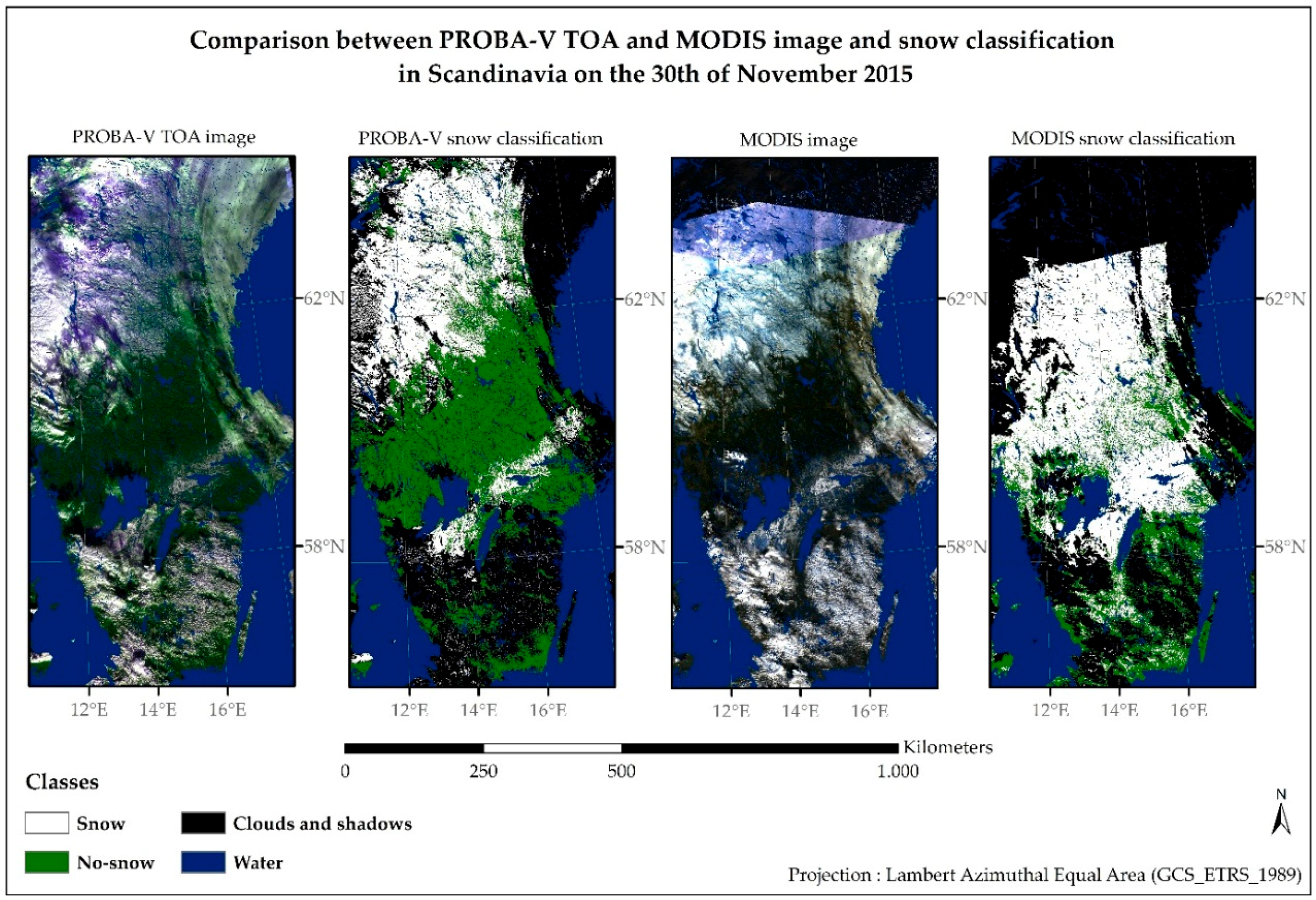
To our knowledge, there are no studies about the specific classification of snow at high SZA with optical sensors. Acomparison between the well-known MOD10A1 snow product and PROBA-V snow classification has therefore been realized. It shows that the snow classification with PROBA-V is significantly higher than MODIS at these SZA. Underestimation of the no snow class and omission errors in the snow class (due to misclassification as clouds) in the MODIS snow product (Table 5) are primary causes for this result. However, three other factors could impact the differences observed between the two snow classifications. First, the classification that has been developed here with PROBA-V is applied at a global scale but is specific and optimized for high SZA snow mapping, while the MOD10A1 snow product has been created to be consistent in a large SZA range and not specifically for high SZA. Indeed, the overall accuracy of MOD10A1 snow product has been assessed by [31] to be between 80% and 100% for a wide range of SZA. However, accuracy was lower for images taken at high SZA. For lower SZA, the MOD10A1 overall accuracy is therefore at least as good as the PROBA-V one. Secondly, the images that have been used in our snow classification are TOA images while Top-Of-Canopy (TOC) images are used in MOD10A1 snow products. In theory, the use of TOC images should lead to a better snow classification in MOD10A1 product, but this was not observed at large SZA. However, it is known that atmospheric corrections at high SZA become challenging. It could be possible that atmospheric corrections at these SZA do not improve the MOD10A1 product anymore. Thirdly, the overpassing time difference between the two satellites induce a variation in the SZA of images. This difference varies between 0.6 and 1° SZA as a function of the date and the latitude. This implies that MODIS images have been taken when the sun was lower than for PROBA-V images. It may lead to an overestimation of the overall accuracy of PROBA-V in comparison with MODIS. However, this variation of SZA is small with respect to the differences in SZA that are investigated and to the low impact of the SZA on the overall accuracy of PROBA-V snow classification.(Figure 5).

The uncertainty (95% confidence intervals) on the overall accuracy estimates was smaller than 5 percent. The uncertainties were also small (<10%) for the producer and the user accuracies of the snow and clouds classes (Table 6). However, uncertainties on user and producer accuracies of the non-snow class are high (up to 44 percent). This is due to the small number of sample points in this class. As a matter of fact, little can be said on these accuracies. The estimated non-snow user accuracy of the PROBA-V classification is larger than MODIS, but this is not statistically significant.

NDSI and NDVI thresholds based on [14,27], which have been used for the snow classification with PROBA-V TOA images, were found to be consistent for the snow classification. Red and NIR band thresholds have been added to avoid classification problems due to low and high spectral values. This increases the quantity of no-data in images, but this is not a major issue as images are captured at a daily basis.

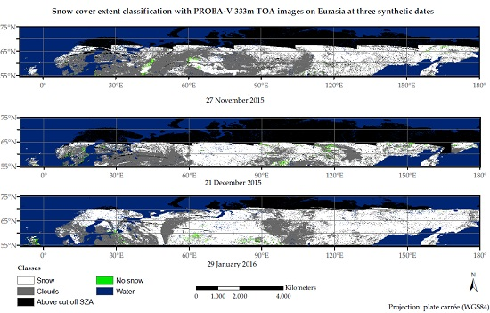
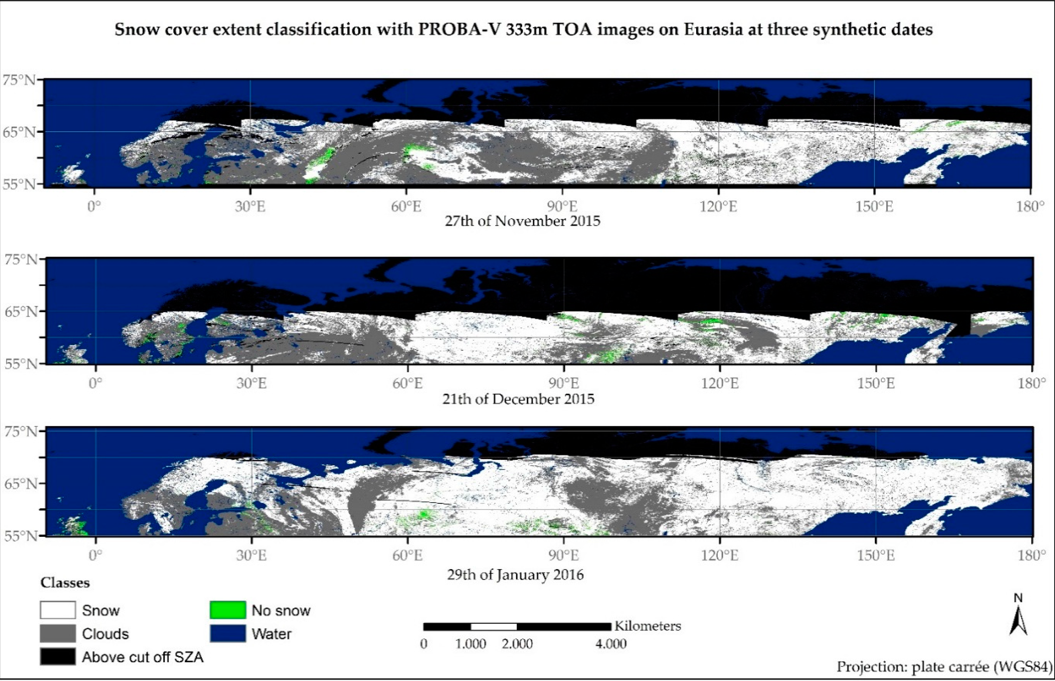
Considering performances of the automated classification even based on TOA images, it seems reasonable to continue image acquisition at least up to 88.5° SZA. Net gain of surface and latitude has been computed based on the maximum SZA of 88.5°, where user and producer accuracies of almost all classes are above 60% (Table 6). The maximum gain of land surface was approximately 11.5 million km² on 18 January 2016 (Figure 8). It represents a bit more than the area of Europe. This large area would be lost every year during winter with the use of previous cut-off angles. This graph is only accurate for winter 2015–2016 because, on one hand, PROBA-V has no onboard propellant, and it is therefore subject to orbital drifting [17]. On the other hand, the maximum latitude gain is a function of the equation of time, which is the astronomical model that describes the difference existing between real and mean solar time. This difference is caused by the tilt of the Earth’s axis and the elliptical orbit of the Earth around Sun [32].The maximum gain of latitude is approximately 8°: it is almost constant between early-November and mid-February. The equation of time does not generate large variations around the latitude values computed for winter 2015–2016.

The large majority of land surface at high latitude are covered with snow during winter. It is therefore important to detect patches of remnant areas without snow. In order to evaluate the interest of snow and no snow maps at high SZA, the probability of remnant no snow areas need to be considered. As [23] and our results show that MOD10 overestimates snow cover at large SZA (Figure 7), the probability of no snow for the different SZA classes was estimated for this winter using the random sample points.

Table 7. Percentages of observed no snow pixels and no snow/snow ratios of the SZA classes used in the validation.

SZA	Percentage of Observed No Snow Pixels	Percentage of No Snow Per Valid Observations
SZA < 81°	11	26
81° < SZA < 85°	7	15
85° < SZA < 87°	3	6
87° < SZA < 88°	2	3
88° < SZA < 88.5°	1	2
88.5° < SZA < 89°	0	0
89° < SZA < 89.5°	0	0

shows that the absence of snow cover is observed with SZA as high as 88.5°. This value is likely to be underestimated because the change of cut-off angle was only effective on 27 October 2015, while its impact on the observed region starts in early October. Due to the lower snow cover probability at the beginning of the season, one could indeed expect to observe more snow cover absence during this period. Furthermore, General Circulation Models (GCMs) predict that the effects of anthropogenic greenhouse warming will be amplified in the northern high latitudes due to feedback in which variations in snow and sea ice extent play key roles [33]. Future snow cover proportions at high latitudes could therefore be affected. This could require the monitoring of snow cover above 88.5° SZA even if, during the winter of 2015–2016, regions above the latitude corresponding to 88.5° SZA were fully covered by snow.

In the specific context of snow cover mapping at high latitude, the confusion between snow and clouds has a lesser impact on the product fitness-to-purpose than the discrimination between vegetation and snow. The probability to observe snow under clouds is indeed very high. The algorithm that has been used is very fast and sufficiently accurate for the purpose of the study. A non-parametric separability analysis [34] was used to assess the potential of PROBA-V to discriminate classes. This analysis yields the probability of the discrimination error between two classes considering the same probability of occurrences. The results of the separability analysis of the different bands show that the probability of misclassification is about 20% for our indices (Figure 9). Therefore, the highest accuracy of classification is about 80% with those indices and observation conditions (SZA, sensor, etc.). The lower probability of misclassification is 10% only for the class no snow—clouds using the red band. The snow classification could therefore not be greatly improved thanks to another algorithm. Nevertheless, the results of the threshold-basedclassification are consistent and proved to be better than MOD10.

The improvement of the snow classification would require further work on atmospheric corrections, which would improve radiometric quality. As we have seen, data between 81° SZA and 88.5° SZA bring useful information on a qualitative point of view (a snow classification is a qualitative information about land cover). Moreover, spaceborne sensors are constantly improving their capabilities in the treatment of low signal-to-noise ratio images. To our knowledge, problems that limit the use of atmospheric corrections at high SZA (above 82°) are the computation time, the lack of remote sensing data at these SZA, and the error introduced when assuming a plane parallel atmosphere. By managing these limitations, the acquisition of data at high SZA could therefore not only be useful for qualitative purposes like classifications but also for quantitative ones like albedo measurements. However, new developments would be impossible without test data at high SZA.

5. Conclusions

In this study, Top Of Atmosphere images at 333 m spatial resolution and daily temporal resolution from PROBA-V have been used to classify snow at very high latitudes (i.e., very high solar zenith angles). This was made possible by the change of cut-off angle of PROBA-V from 82° to 90° of solar zenith angle. To our knowledge, snow classification with optical images has never been realized at such high solar zenith angles. The overall accuracy of the snow classification is 81.1% ± 4% and user and producer accuracies are above 70% and have small confidence intervals (except for the no snow class) at least up to 88.5° of solar zenith angle. The snow classification has been compared to the MOD10A1 snow product and showed better results as the overall accuracy of the latter is 75% ± 4% at these SZA. Moreover, all producer and user accuracies of our snow classification except the producer accuracy of the clouds class were above MOD10A1.

This study demonstrates that it is both relevant and technically possible to use optical remote sensing images to map snow at solar zenith angles of at least 88.5°. Above this SZA, the classification accuracy is affectedd by chromatic aberrations, high atmospheric diffusion and aerosol scattering and low signal-to-noise ratio.

Considering the relevance of snow cover mapping for ecology and climatology, more information should be derived from optical Earth Observation satellites at high latitude by changing this cut-off angle. In addition to representing a clear added value to the mission, this change would basically have no cost (apart of downlink capacity) and no impact on other applications.

References

1. Robinson, D.A.; Frei, A. Seasonal variability of northern hemisphere snow extent using visible satellite data. Prof. Geogr. 2000. [Google Scholar] [CrossRef]
2. Frei, A.; Tedesco, M.; Lee, S.; Foster, J.; Hall, D.K.; Kelly, R.; Robinson, D.A. A review of global satellite-derived snow products. J. Adv. Space Res. 2012. [Google Scholar] [CrossRef]
3. Barnett, T.P.; Adams, J.C.; Lettenmeier, D.P. Potential impacts of a warming climate on water availability in snow-dominated regions. Nature 2005. [Google Scholar] [CrossRef] [PubMed]
4. Peterson, B.J.; Holmes, R.M.; McClelland, J.W.; Vörösmarty, C.J.; Lammers, R.B.; Shiklomanov, I.A.; Rahmstorf, S. Increasing river discharge to the Arctic Ocean. Science 2002, 298, 2171–2173. [Google Scholar] [CrossRef] [PubMed]
5. Barnett, T.P.; Dümenil, L.; Schlese, U.; Roeckner, E.; Latif, M. The effect of Eurasian snow cover on regional and global climate variations. J. Atmos. Sci. 1989, 46, 661–685. [Google Scholar] [CrossRef]
6. Boyd, H.; Petersen, A. Spring arrivals of migrant waders in Iceland in the 20th century. Ringing Migr. 2006. [Google Scholar] [CrossRef]
7. Bienau, M.J.; Hattermann, D.; Kröncke, M.; Kretz, L.; Otte, A.; Eiserhardt, W.L.; Milbau, A.; Graae, B.J.; Durka, W.; Eckstein, R.L. Snow cover consistently affects growth and reproduction of Empetrum hermaphroditum across latitudinal and local climatic gradients. Swiss Bot. Soc. 2014, 124, 115–129. [Google Scholar] [CrossRef]
8. Hansson, L.; Henttonen, H. Gradients in density variations of small rodents: The importance of latitude and snow cover. Oecologia 1985, 67, 394–402. [Google Scholar] [CrossRef]
9. Hein, N.; Feilhauer, H.E.; Finch, O.-D.; Schmidtlein, S.; Ler, J.L. Snow cover determines the ecology and biogeography of spiders (Aranae) in alpine tundra ecosystems. Erdkunde 2014, 68, 157–172. [Google Scholar] [CrossRef]
10. Boggs, C.L.; Inouye, D.W. A single climate driver has direct and indirect effects on insect population dynamics. Ecol. Lett. 2012, 15, 502–508. [Google Scholar] [CrossRef] [PubMed]
11. Wipf, S.; Rixen, C. A review of snow manipulation experiments in Arctic and alpine tundra ecosystems. Polar Res. 2010, 29, 95–109. [Google Scholar] [CrossRef]
12. Helfrich, S.R.; McNamara, D.; Ramsay, B.H.; Baldwin, T.; Kasheta, T. Enhancements to, and forthcoming developments in the Interactive Multisensor Snow and Ice Mapping System (IMS). Hydrol. Process. 2007, 21, 1576–1586. [Google Scholar] [CrossRef]
13. Metsämäki, S.; Saliminen, M.; Pulliainen, J.; Luojus, K.; Nagler, T.; Bippus, G.; Solberg, R.; Salberg, A.-B.; TRIER, Ø.D.; Wiesmann, A. Global Snow Monitoring for Climate Research, Algorithm Theoretical Basis Document. 2013. Available online: http://www.globsnow.info/docs/GS2_SWE_ATBD.pdf (accessed on 22 April 2016).
14. Hall, D.K.; Riggs, G.A.; Salomonson, V.V.; Barton, J.S.; Casey, K.; Chien, J.Y.L.; DiGirolamo, N.E.; Klein, A.G.; Powell, H.W.; Tait, A.B. Algorithm Theoretical Basis Document (ATBD) for the MODIS Snow and Sea Ice-Mapping Algorithms. 2001. Available online: http://modis.gsfc.nasa.gov/data/atbd/atbd_mod10.pdf (accessed on 22 April 2016). [Google Scholar]
15. Klein, A.G.; Hall, D.K.; Riggs, G.A. Improving snow cover mapping in forests through the use of a canopy reflectance model. Hydrol. Process. 1998, 12, 1723–1744. [Google Scholar] [CrossRef]
16. Zhu, Z.; Woodcock, C.E. Improvement and Expansion of the Fmask Algorithm: Cloud, Cloud Shadow, and Snow Detection for Landsats 4–7, 8, and Sentinel 2 images. Remote Sens. Environ. 2014, 159, 269–277. [Google Scholar] [CrossRef]
17. Dietz, A.J.; Kuenzer, C.; Gessner, U.; Dech, S. Remote sensing of snow—A review of available methods. Int. J. Remote Sens. 2012, 33, 4094–4134. [Google Scholar] [CrossRef]
18. ESA Sentinel Online. Available online: https://sentinel.esa.int/web/sentinel/technical-guides/sentinel-2-msi/level-2a/algorithm (accessed on 22 April 2016).
19. Wolters, E.; Dierckx, W.; Dries, J.; Swinnen, E. PROBA-V Products User Manual v1.1. 2014. Available online: http://proba-v.vgt.vito.be/sites/default/files/Product_User_Manual.pdf (accessed on 22 April 2016).
20. Leroy, J.-L. La Polarisation de la Luzmière et L’observation Astronomique; Gordon and Breach Science Publishers: Amsterdam, The Netherlands, 1998; pp. 32–33. [Google Scholar]
21. Stroeve, J.; Box, J.E.; Gao, F.; Liang, S.; Nolin, A.; Schaaf, C.B. Accuracy assessment of the MODIS 16-day albedo product for snow: Comparisons with Greenland in situ measurements. Remote Sens. Environ. 2005. [Google Scholar] [CrossRef]
22. Kajiwara, K.; Tateishi, R.; Mastumoto, M. Correction of solar Zenith Angle effect of NOAA AVHRR data for global monitoring. In Proceedings of the Asian Conference on Remote Sensing (ACRS), Singapore, 30 October–5 November 1991.
23. Riggs, G.; Hall, D.K. MODIS snow and ice products, and their assessment and applications. Land Remote Sens. Glob. Environ. Chang. 2011, 11, 681–707. [Google Scholar]
24. Dierckx, W.; Sterckx, S.; Benhadj, I.; Livens, S.; Duhoux, G.; Van Achteren, T.; Francois, M.; Mellab, K.; Saint, G. PROBA-V mission for global vegetation monitoring: Standard products and image quality. Int. J. Remote Sens. 2014, 35, 2589–2614. [Google Scholar] [CrossRef]
25. VITO. Available online: http://www.vito-eodata.be/PDF/portal/Application.html (accessed on 22 April 2016).
26. Defourny, P.; Kirches, G.; Brockmann, C.; Boettcher, M.; Peters, M.; Bontemps, S.; Lamarche, C.; Schlerf, M.; Santoro, M. Land Cover CCI Algorithm Theoretical Basis Document v2.5; UCL-Geomatics: Louvain-la-Neuve, Belgium, 2016; pp. 54–62. [Google Scholar]
27. Weier, J.; Herring, D. Measuring Vegetation (NDVI & EVI). Available online: http://earthobservatory.nasa.gov/Features/MeasuringVegetation/ (accessed on 22 April 2016).
28. Liu, C.; Frazier, P.; Kumar, L. Comparative assessment of the measure of thematic classification accuracy. Remote Sens. Environ. 2007, 107, 606–616. [Google Scholar] [CrossRef]
29. Congalton, R.; Green, K. Thematic accuracy. In Assessing the Accuracy of Remotely Sensed Data: Principles and Practices, 2nd ed.; CRC press: New York, NY, USA, 2009; pp. 55–61. [Google Scholar]
30. Strahler, A.H.; Boschetti, L.; Foody, G.M.; Friedl, M.A.; Hansen, M.C.; Herold, M.; Mayaux, P.; Morisette, J.T.; Stehman, S.V.; Woodcock, C.E. Global Land Cover Validation: Recommendations for Evaluation and Accuracy Assessment of Global Land Cover Maps; GOFC-GOLD Report; Office for Official Publications of the European Communities: Luxembourg, 2006; Volume 25, pp. 1–52. [Google Scholar]
31. Simic, A.; Fernandes, R.; Brown, R.; Romanov, P.; Park, W. Validation of VEGETATION, MODIS, and GOES + SSM/I snow-cover products over Canada based on surface snow depth observations. Hydrol. Process. 2004, 18, 1089–1104. [Google Scholar] [CrossRef]
32. Duffett-Smith, P. Practical Astronomy with Your Calculator; Cambridge University Press: Cambridge, UK, 1988; pp. 98–99. [Google Scholar]
33. Serreze, M.C.; Walsh, J.E.; Chapin, F.S.; Osterkamp, T.; Dyurgerov, M.; Romanovsky, V.; Oechel, W.C.; Morison, J.; Zhang, T.; Barry, R.G. Observational Evidence of recent change in the northern high-latitude environment. Clim. Chang. 2000, 46, 159–207. [Google Scholar] [CrossRef]
34. Radoux, J.; Chomé, G.; Jacques, D.C.; Waldner, F.; Bellemans, N.; Matton, N.; Lamarche, C.; d’Andrimont, R.; Defourny, P. Sentinel-2’s Potential for Sub-Pixel landscape feature detection. Remote Sens. 2016, 8, 488. [Google Scholar] [CrossRef]
Figure 1. Scheme of the snow classification processing chain of Sentinel-2. Source: [18].
Remotesensing 08 00699 g001
Figure 2. Representation of the impact of high Sun Zenith Angle SZA on shadows (no incident light) in a part of Scandinavia. The SZA in the center of the subsets is equal to 47.5° on 21 June 2015 and to 87.25° on the 21 December 2015 at the PROBA-V overpass time.
Remotesensing 08 00699 g002
Figure 3. Snow cover extent classification with PROBA-V 333 m top-of-atmosphere images on North America and Greenland at three synthetic dates.
Remotesensing 08 00699 g003
Figure 4. Snow cover extent classification with PROBA-V 333 m top-of-atmosphere images on Eurasia at three synthetic dates.
Remotesensing 08 00699 g004
Figure 5. Overall accuracy of the snow cover classification for the different sun zenith angles classes.
Remotesensing 08 00699 g005
Figure 6. Evolution of the producer and user accuracy of the snow cover class with sun zenith angle and their confidence intervals at 95%.
Remotesensing 08 00699 g006
Figure 7. Comparison between a PROBA-V true color image and a MODIS image of a part of Scandinavia on 30 November 2015 (SZA between 79° and 88.5°) and their respective snow classifications.
Remotesensing 08 00699 g007
Figure 8. Evolution of the gain in terms of surface (blue) and decimal degree of latitude (red) during winter 2015–2016 due to the change from 82° to 90° sun zenith angle SZA. The asymmetry of gain for both curves is due to the equation of time.
Remotesensing 08 00699 g008
Figure 9. Probability of misclassification (classification error) of major classification classes for different indices of separation. Red, Near InfraRed (NIR), Blue and Short Wave InfraRed (SWIR) correspond to the four bands of PROBA-V, Normalized Difference Vegetation Index (NDVI) and Normalized Difference Snow Index (NDSI) are the two indices used in our classification, simple Ratio (SR) BlueRed is the index used in Sentinel-2 snow classification (Figure 1) and S3 to S5 are indices used in the PROBA-V snow quality flag (Table 1).
Remotesensing 08 00699 g009