Article

Assessing the Severity of Wind Gusts with Lidar

Wind Energy Research Group, Faculty of Aerospace Engineering, Delft University of Technology, Kluyverweg 1, Postbus 5058, 2600 GB Delft, The Netherlands
*
Author to whom correspondence should be addressed.
Remote Sens. 2016, 8(9), 758; https://doi.org/10.3390/rs8090758
Submission received: 12 July 2016 / Revised: 2 September 2016 / Accepted: 8 September 2016 / Published: 14 September 2016
(This article belongs to the Special Issue Remote Sensing of Wind Energy)

Abstract

:
Lidars have gained a lot of popularity in the field of wind energy, partly because of their potential to be used for wind turbine control. By scanning the oncoming wind field, any threats such as gusts can be detected early and high loads can be avoided by taking preventive actions. Unfortunately, lidars suffer from some inherent weaknesses that hinder measuring gusts; e.g., the averaging of high-frequency fluctuations and only measuring along the line of sight). This paper proposes a method to construct a useful signal from a lidar by fitting a homogeneous Gaussian velocity field to a set of scattered measurements. The output signal, an along-wind force, acts as a measure for the damaging potential of an oncoming gust and is shown to agree with the rotor-effective wind speed (a similar control input, but derived directly from the wind turbine’s shaft torque). Low data availability and the disadvantage of not knowing the velocity between the lidar beams is translated into uncertainty and integrated in the output signal. This allows a designer to establish a control strategy based on risk, with the ultimate goal to reduce the extreme loads during operation.

Graphical Abstract

1. Introduction

There has been a lot of interest in using lidar for wind energy in the recent years, for example to assess the energy yield on a site or to validate a turbine’s power curve. Another very promising application is in the form of lidar-assisted control systems to reduce the loads on turbines during operation. Such systems use a lidar to scan the oncoming wind field to obtain information on the velocity field. Knowing what to expect allows a controller to anticipate any strong perturbations (e.g., gusts), for instance by preventively lowering the thrust on the rotor by pitching the blades. This is different from the conventional feedback controllers used presently, which operate by regulating the generator torque and speed with the big disadvantage that they can only react to past events. Severe gusts, with the potential to trigger extreme loads, can therefore only be dealt with after they have hit the rotor. The potential of lidar-assisted control for the reduction of fatigue and extreme loads is recognized in multiple studies [1,2,3,4]. A study by Schlipf et al. [5] showed a 51% reduction in loads resulting from an extreme operating gust as prescribed by the International Electrotechnical Commission (IEC) [6]. Although the study was performed with a uniform velocity field—not necessarily representative of a real-life event—it shows that lidar-assisted controllers have great potential for gust control when given the proper input.
Although lidars are generally regarded as being suitable tools to assess the mean wind speed, they suffer from some inherent weaknesses that hinder the measurement of gusts. Doppler lidar systems operate by sending out a laser beam and measuring the Doppler shift as the light scatters back from the natural aerosols. Wind speeds are normally averaged along the length of the pulse by range weighting, thereby losing information about the high frequencies. Moreover, lidars are inherently confronted by the so-called cyclops dilemma [7], meaning that only the wind speed component along the line of sight can be measured. In addition, nacelle-mounted lidars can be plagued by low data availability, for instance due to the passing of the blades in front of the lens. These issues are addressed in several studies that focus on using lidar measurements to obtain mean wind and turbulence properties [8,9,10,11] or achieve real-time wind field construction [12].
However, what a controller ultimately wants to use is one or a set of inputs that have a direct impact on the performance of the entire rotor disk. This is why some authors prefer a rotor-effective or blade-effective wind speed [13,14,15] instead of the full velocity field. Therefore, in order to make any decision on what action to take in response to an oncoming threat, one requires a method to turn a set of (possibly scattered) measurements into useful information. In addition, the inherent weaknesses of the lidar induce some degree of uncertainty, which needs to be taken into account.
In this paper, we propose a method to assess the severity of an oncoming gust. This is done by fitting a homogeneous Gaussian velocity field to a set of scattered point measurements, of which the statistics can be derived analytically. The velocity field allows one to predict the along-wind force acting on the rotor area, which is a measure of the damaging potential of a gust and can be used as control input. Additionally, the uncertainty coming from only knowing the velocity along the lidar beams can be included with the along-wind force in a straightforward fashion. The method is demonstrated by an example of a gust measured in the field by a pulsed lidar system mounted on the nacelle of a 5 MW wind turbine. Furthermore, we validate the outcome by comparing the resulting along-wind force with the rotor-effective wind speed, which is a signal derived from the turbine’s shaft torque and is considered representative for the rotor thrust force.

2. Methods

2.1. Lidar Set-Up

The set-up consists of an Avent-Lidar five-beam prototype pulsed lidar system mounted on the nacelle of a Darwind XD115-5MW wind turbine (XEMC Darwind B.V., Hilversum, The Netherlands), having a rotor diameter of 115 m and a hub height of 100 m. The turbine is located at the test field of the Energy Research Centre of the Netherlands (ECN) in the Wieringermeer polder, surrounded by flat homogeneous terrain.
The lidar provides measurements at 10 range gates simultaneously, from 50 to 185 m upwind (see Figure 1). It samples the velocity along five beam positions every 1.25 s (changing position every 0.25 s). Next to a center beam position (0), there are four beam positions (1–4) that make a 15 angle with respect to the horizontal plane.

2.2. The Velocity Field around Measurement Points

The lidar averages the velocities over the beam path. For a pulsed lidar in particular, this can be modeled by a Gaussian pulse shape [16]. The velocities at a distance, r, measured by the range gate at R, are then weighted according to
w ( r ) = 1 2 Δ R erf R r + 1 2 Δ R Δ Z erf R r 1 2 Δ R Δ Z ,
where Δ R is the spacing between the range gates, Δ Z is the e 1 radius of the pulse, and erf ( x ) is the error function. The e 1 radius of the pulse is derived from the full-width-at-half-maximum pulse width (FWHM):
Δ Z = FWHM 2 ln 2 ,
where FWHM = 30 m for the set up used in this paper. If the streamwise component of the wind speed is much larger than the lateral and vertical components (i.e., u v , w ), the line-of-sight velocity measured at the point x j = x j , y j , z j T is
u LOS , j cos φ j u ( x j + r , y j , z j ) w ( r ) d r ,
where φ is the beam angle. The velocity error (or directional bias) included with the u-component is given by [15]:
ϵ u = tan φ v sin ψ w cos ψ ,
where ψ is the lidar azimuth angle. For example, on an IEC class A site [6] and φ = 15 , the root-mean-squared error with respect to the longitudinal component is on the order of 5% at a ten-minute mean wind speed of u ¯ = 4 m/s, decreasing to 3% at u ¯ = 12 m/s. The error can be significant when the v- or w-components are significant (e.g., at lower wind speeds, in an unstable atmosphere, or when using larger beam angles). Still, for wind turbines in particular it should be manageable, considering that the relevant extreme loads are generally found at and around the rated wind speeds (on the order of 10–12 m/s) and often under neutral atmospheric conditions.
Assuming that the points x 1 , , x n advect downstream unchanged with the mean wind speed, the result is a domain with n scattered measurements over a certain time period (see Figure 2). Based on this, the surrounding velocities are part of a conditional field given by
u ^ ( x ) = u ( x ) | u ( x 1 + r , y 1 , z 1 ) w ( r ) d r = u LOS , 1 cos φ 1 , , u ( x n + r , y n , z n ) w ( r ) d r = u LOS , n cos φ n ,
where u = u , v , w T is the velocity vector.
The turbulent wind field is highly random in nature and a full three-dimensional velocity field cannot be captured by the lidar. Still, it is possible to rely on statistics and cross-correlations in order to make the best estimate for the space between the measurement points. The idea is that the spectral characteristics of a homogeneous velocity field (including randomly spawned gusts) can be described by the spectral tensor:
Φ ( κ ) = 1 ( 2 π ) 3 R ( r ) e i κ · r d r ,
which is the Fourier transform of the covariance tensor:
R ( r ) = E u ( x ) u ( x + r ) E u ( x ) v ( x + r ) E u ( x ) w ( x + r ) E v ( x ) u ( x + r ) E v ( x ) v ( x + r ) E v ( x ) w ( x + r ) E w ( x ) u ( x + r ) E w ( x ) v ( x + r ) E w ( x ) w ( x + r ) .
The theory behind this is well-established (e.g., see [17]), and many spectral models for boundary-layer atmospheric turbulence exist in literature [18].
As long as u ^ ( x ) is homogeneous and Gaussian distributed around the mean, u ¯ ( x ) , it is possible to estimate this field as:
u ^ ( x ) = u ¯ ( x ) + κ C ( κ ) n ^ ( κ ) e i κ · x ,
where κ = κ x , κ y , κ z T is the wave number vector. The matrix, C , can be derived from the spectral tensor by:
C ( κ ) C * ( κ ) = Δ κ Φ ( κ κ ) d κ ,
with * denoting a conjugate transpose. Moreover, n is a white noise vector that is distributed according to a circularly symmetric complex normal distribution, CN ( 0 , I ) ; i.e.,
Re ( n ) Im ( n ) N 0 0 , 1 2 I 0 0 I .
Since Equation (8) is a straightforward summation, it can easily be replaced by a matrix-vector product:
u ^ ( x ) u ¯ ( x ) = Ψ n ^ ,
where
Ψ = , C ( κ j 1 ) e i κ j 1 · x , C ( κ j ) e i κ j · x , C ( κ j + 1 ) e i κ j + 1 · x , ,
n ^ = n ^ ( κ j 1 ) n ^ ( κ j ) n ^ ( κ j + 1 ) .
The streamwise velocity component follows in a similar fashion from the first row of the matrix Ψ:
u ^ ( x ) u ¯ ( x ) = Ψ u n ^ ,
where
Ψ u = , C u u ( κ j ) , C u v ( κ j ) , C u w ( κ j ) e i κ j · x , .
Then, on the basis of a set of n point measurements of the horizontal wind speed, contained in the vector
b = u LOS , 1 / cos φ 1 u ¯ ( x 1 ) u LOS , 2 / cos φ 2 u ¯ ( x 2 ) u LOS , n / cos φ n u ¯ ( x n ) ,
the vector n ^ that satisfies (5) follows from a conditional distribution:
n ^ = n | Y n = b ,
where Y is constructed from the matrix Ψ u (15):
Y = , W ( κ x , j ) C u u ( κ j ) , C u v ( κ j ) , C u w ( κ j ) e i κ j · x 1 , , W ( κ x , j ) C u u ( κ j ) , C u v ( κ j ) , C u w ( κ j ) e i κ j · x 2 , , W ( κ x , j ) C u u ( κ j ) , C u v ( κ j ) , C u w ( κ j ) e i κ j · x n , ,
where W ( κ x ) is the Fourier transform of the range-weighting function, w ( r ) . Because n ^ is assumed to be Gaussian, its statistics are given by
n ^ N Y * Y Y * 1 b , I Y * Y Y * 1 Y ,
with Y * Y Y * 1 being the right (pseudo) inverse of Y . This means that the statistics of the velocity field u ^ ( x ) follow in a straightforward fashion from Equations (12) and (19):
E u ^ ( x ) = E u ¯ ( x ) + Ψ E n ^ ,
     E u ^ ( x ) = u ¯ ( x ) + Ψ Y * Y Y * 1 b ,
   var u ^ ( x ) = var u ¯ ( x ) + Ψ var n ^ Ψ * ,
    var u ^ ( x ) = Ψ Ψ * Ψ Y * Y Y * 1 Y Ψ * .

2.3. An Expression for the Risk of Severe Wind Gusts

An often-used simplification for gusts is Taylor’s frozen turbulence hypothesis, which assumes that a gust structure remains unchanged over a certain sampling period. This has been shown to hold for at least the low wave numbers [19] (containing the majority of the momentum). With only streamwise advection (i.e., u ¯ = u ¯ , 0 , 0 T ), the momentum balance in x-direction is then
ρ u ¯ u x = p x ,
where p / x is the streamwise pressure gradient and ρ the air density. This leads to
x ρ u ¯ u + p = 0 ,
and eventually results in
p + ρ u ¯ u = const ,
with the constant being the stagnation pressure. The force applied to a plane A, perpendicular to the flow, can be found by integrating the dynamic pressure term, ρ u ¯ u :
F ( r ) = ρ A u ¯ ( r , y , z ) u ( r , y , z ) d y d z ,
where F is used to denote the along-wind force at a distance r upwind (i.e., the rate at which momentum is advected through the plane A).
This along-wind force, in essence proportional to a weighted dynamic pressure, is seen in other fields as well. In aerospace engineering (rocketry in particular), the maximum stresses experienced by a structure in a flight envelope is often linked to the point of maximum dynamic pressure, referred to as the “max Q”. For wind turbines, this could be a very simple yet effective way of expressing the damaging potential of an oncoming gust (see Figure 3). Irrespective of what happens at the rotor plane, the force F is directly connected to the structural loads. In addition, since the frozen turbulence assumption prevents any squared velocity terms from occuring in Equation (27), it follows that F is also Gaussian distributed. It is then straightforward to incorporate the uncertainty on the basis of an estimated streamwise velocity field, u ^ ( x ) :
E F ^ ( r ) = ρ A u ¯ ( r , y , z ) E u ^ ( r , y , z ) d y d z ,
   var F ^ ( r ) = ρ 2 A A u ¯ 2 ( r , y , z ) var u ^ ( r , y , z ) d y d z .

3. Results

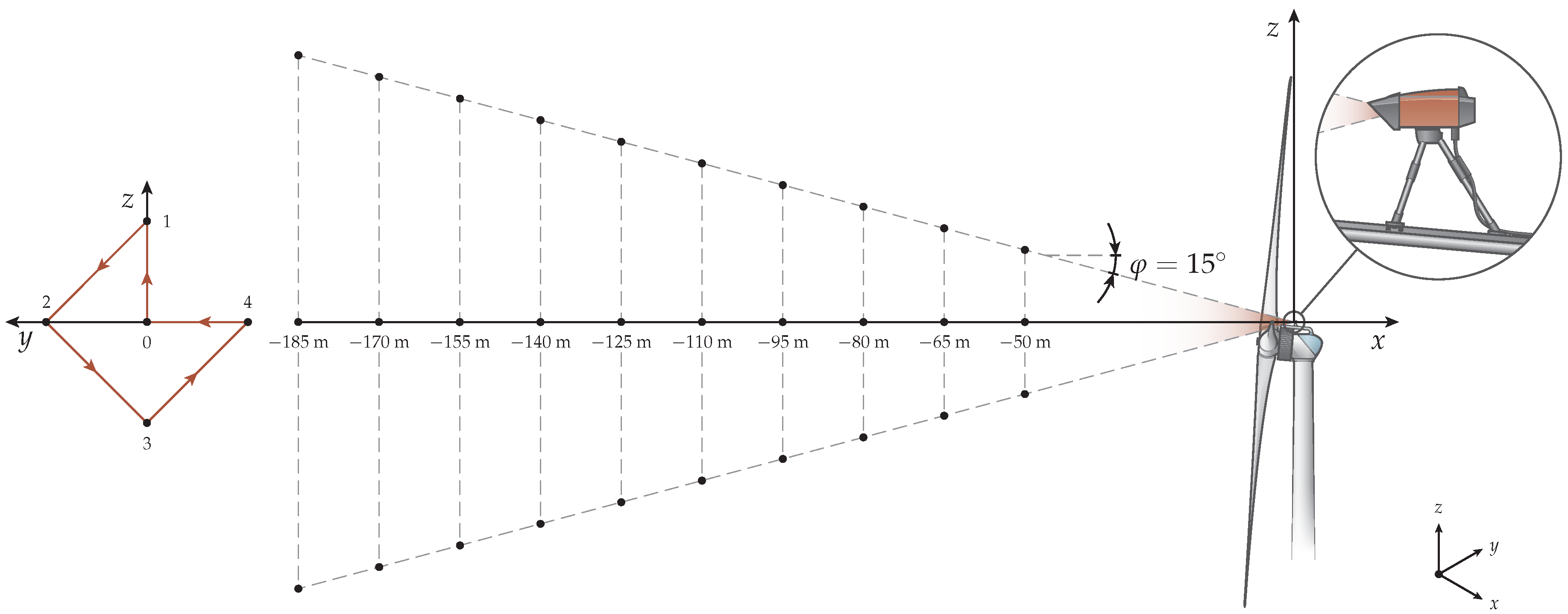
The example shown in this section is based on a 17 m/s velocity peak ( u ¯ + 5 σ u ) measured by the center beam at a range of r = 140 m on 22 December 2013. During this time, the turbine was not affected by the wake of neighboring turbines or met masts and was operating under a slight yaw misalignment of 2 . 5 (taken as the difference between the turbine’s yaw angle and the wind direction measured at 97 m height by the neighboring met mast). The ten-minute mean hub height wind speed measured at the r = 140 m range gate was about 13.3 m/s with a longitudinal turbulence intensity of 5.9% (taken directly from the lidar). Considering that the terrain is flat and homogeneous, a neutral wind shear profile was fitted to the ten-minute mean wind speeds measured along beam positions 0, 1, and 3 (again, at r = 140 m):
u ¯ ( z ) = u ¯ ( z ref ) ln z / z 0 ln z / z ref ,
yielding a roughness length of z 0 0 . 55 m, which is representative of the site [
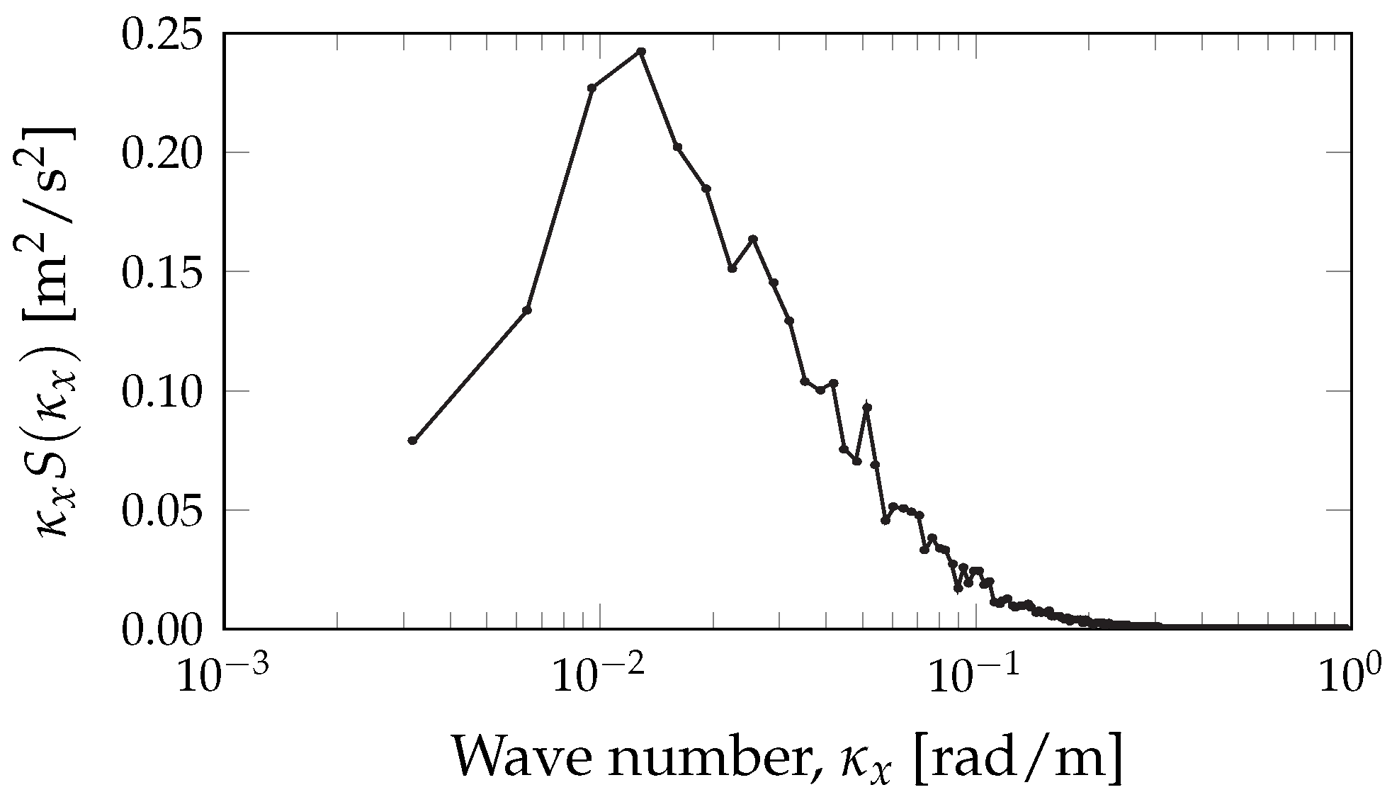
20]. Furthermore, a spectral tensor Φ ( κ ; L , α ϵ 2 / 3 , Γ ) according to [21], was set up with L 25 m, α ϵ 2 / 3 0 . 16 m 4 / 3 /s 2 , and Γ 3 . The length scale was estimated from the average of 12 ten-minute spectra from the preceding two hours (see Figure 4). The α ϵ 2 / 3 parameter was found by scaling the u-component of the spectral tensor to match the ten-minute longitudinal variance along the center beam:
W 2 ( κ x ) Φ u u ( κ ) d κ = σ u , LOS 2 ,
where again the filtering with W denotes the effect of range-weighting. The shear parameter, Γ, was taken from [22] to match neutral atmospheric conditions.
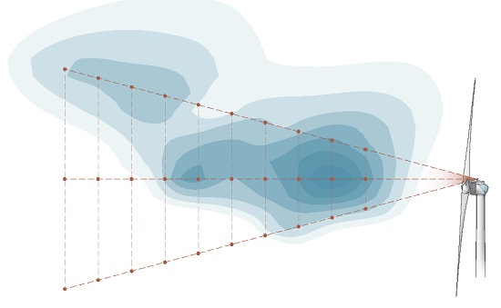
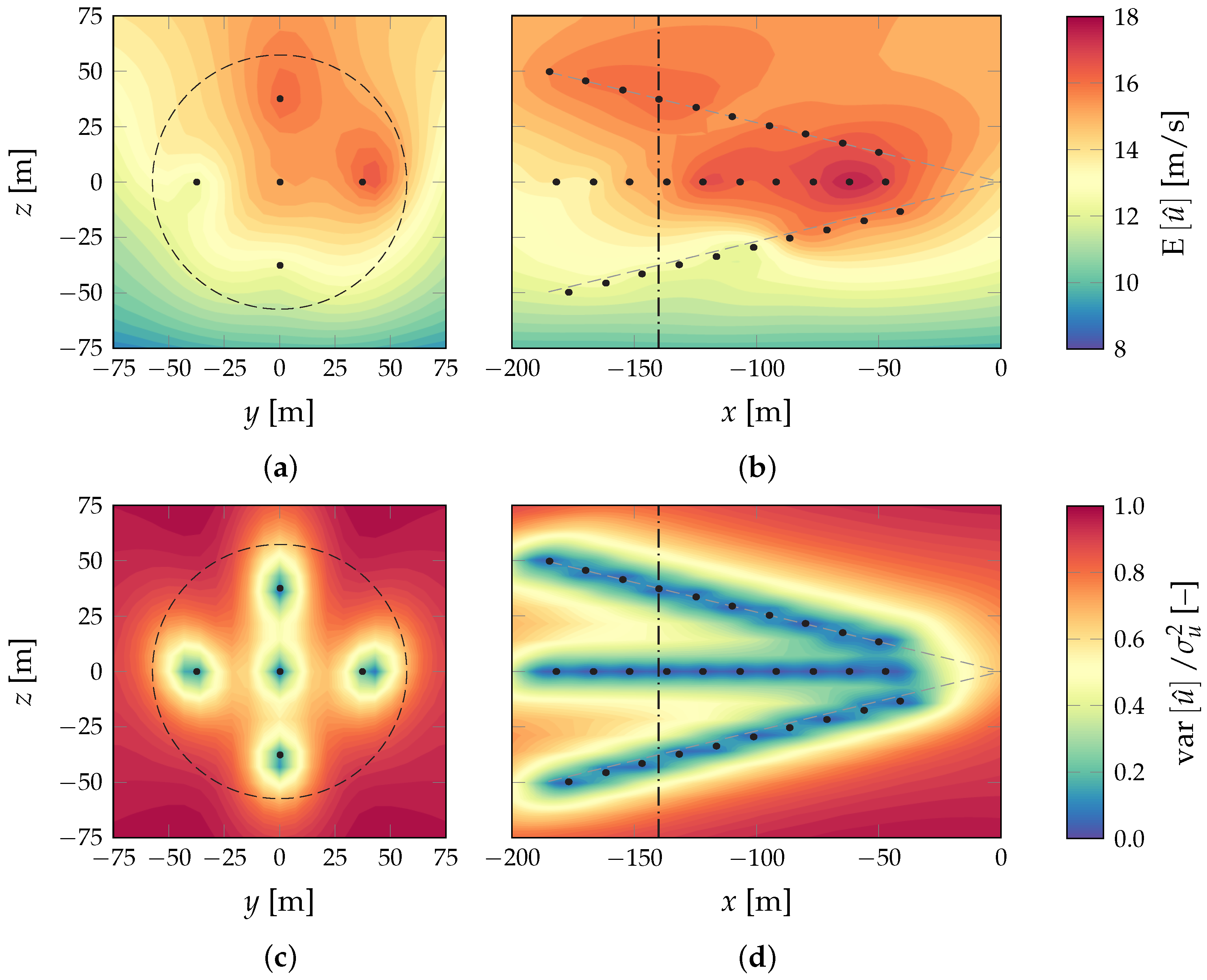
Figure 5 shows slices of the velocity field fitted to one full measurement cycle (10 ranges × 5 beam locations: n = 50 ), at a time where all five beams were available. Figure 5a,c shows a slice of the wind field at a distance r = 140 m. Figure 5b,d shows the x z -plane through y = 0 . Figure 5a,b show that it is possible, even with a collection of scattered points, to make an educated guess of the size of an upcoming gust structure. At the same time, Figure 5c,d are able to show approximately how reliable these estimates are. A variance of var u ^ = 0 implies that the velocity is known for certain, whereas a variance of var u ^ = σ u 2 implies that there is no knowledge about the field but the ten-minute statistics. Of course, the uncertainty is the lowest along the direction of the beam, although it never reaches zero because of range weighting and beam pointing. Figure 5c also shows that the range gate at x = 140 m is a convenient one to rely on, since it provides good coverage of the rotor disk (although all 50 points are used to estimate u ^ ( x ) ).
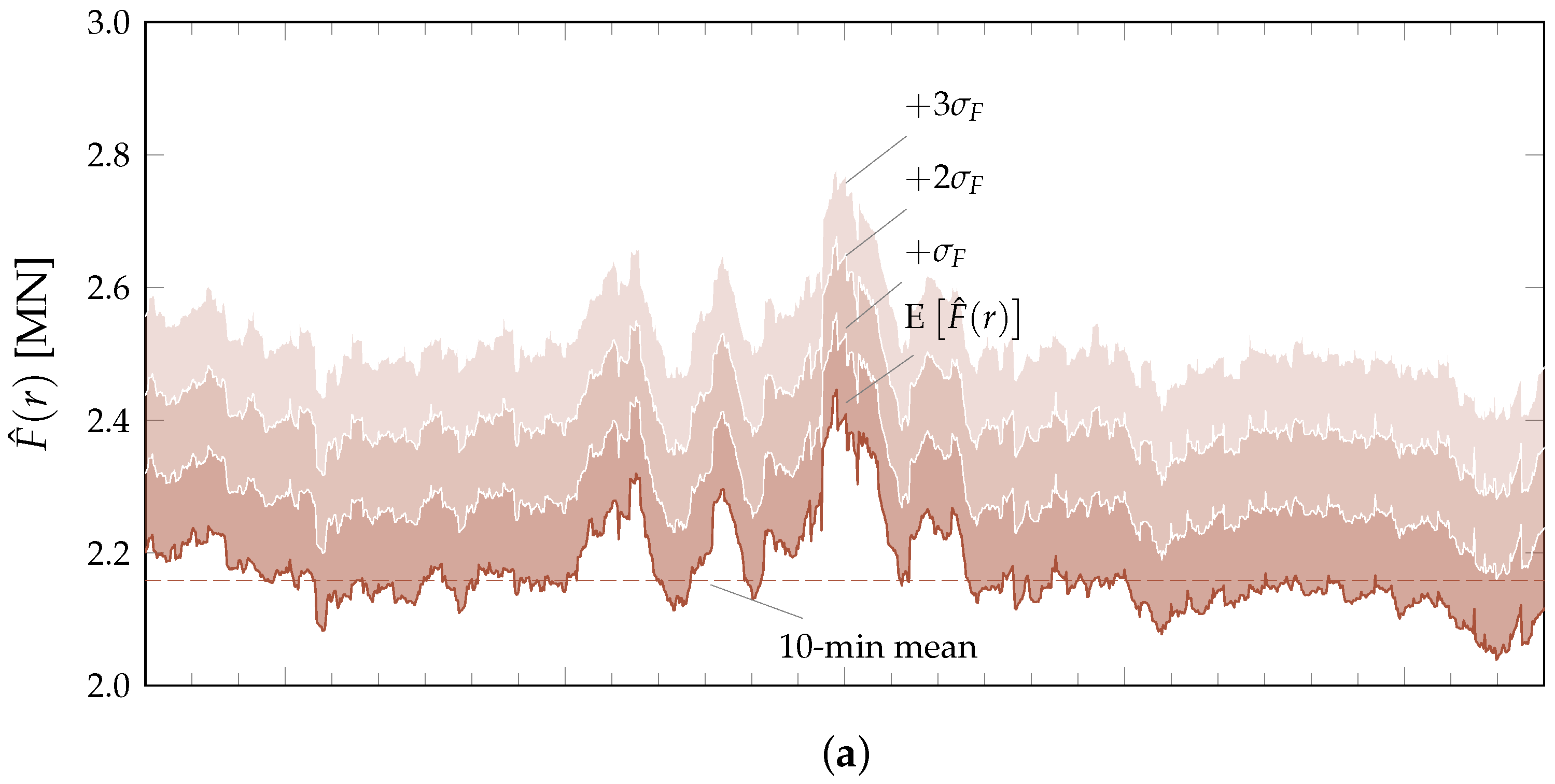
Figure 6 shows how the estimated along-wind force, F ^ , through the disk at r = 140 m is constructed from the individual beam signals. First, Figure 6a shows the expectation plus 1–3 standard deviations, corresponding to an exceedance probability of 15.9%, 2.3%, and 0.1%, respectively. The highest peak of the signal, at t 0 , approximately matches the peaks in the velocity signals, which is what one would expect. The fact that the velocity peaks stay above the mean for a relatively long period (10–20 s) is already an indication that the gust structure is large and contains a lot of momentum. At the same time, very localized peaks, such as u 0 at t = 70 s, hardly have an effect on the total along-wind force.
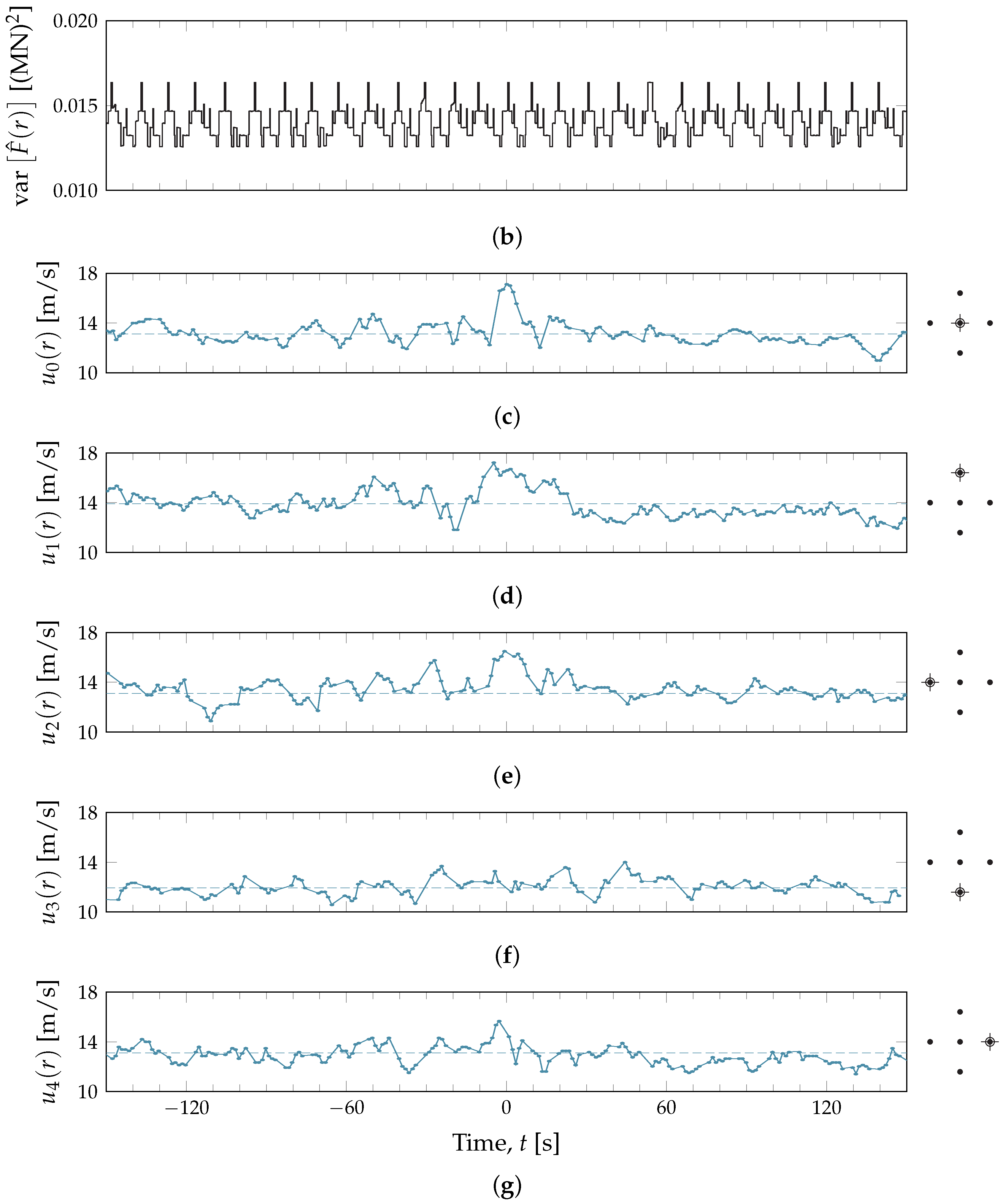
Shown in Figure 6b is the variance associated with F ^ , which is a direct result of the data availability. The lidar can only supply a set of point measurements along several beams and all the space in between is translated into uncertainty. This uncertainty not only includes the probability that a certain measured peak is very local, but also the possibility of another, higher velocity peak being hidden between the beams. It also means that, if the flow is strongly correlated with itself, the quality of the forecast would naturally increase because one point measurement is more representative of its surroundings. Another source of uncertainty is that not all five lidar beams are available every full cycle, which is why the variance fluctuates over time. This is due to the rotor blades passing in front of the beam and the overall technical availability of the lidar system.
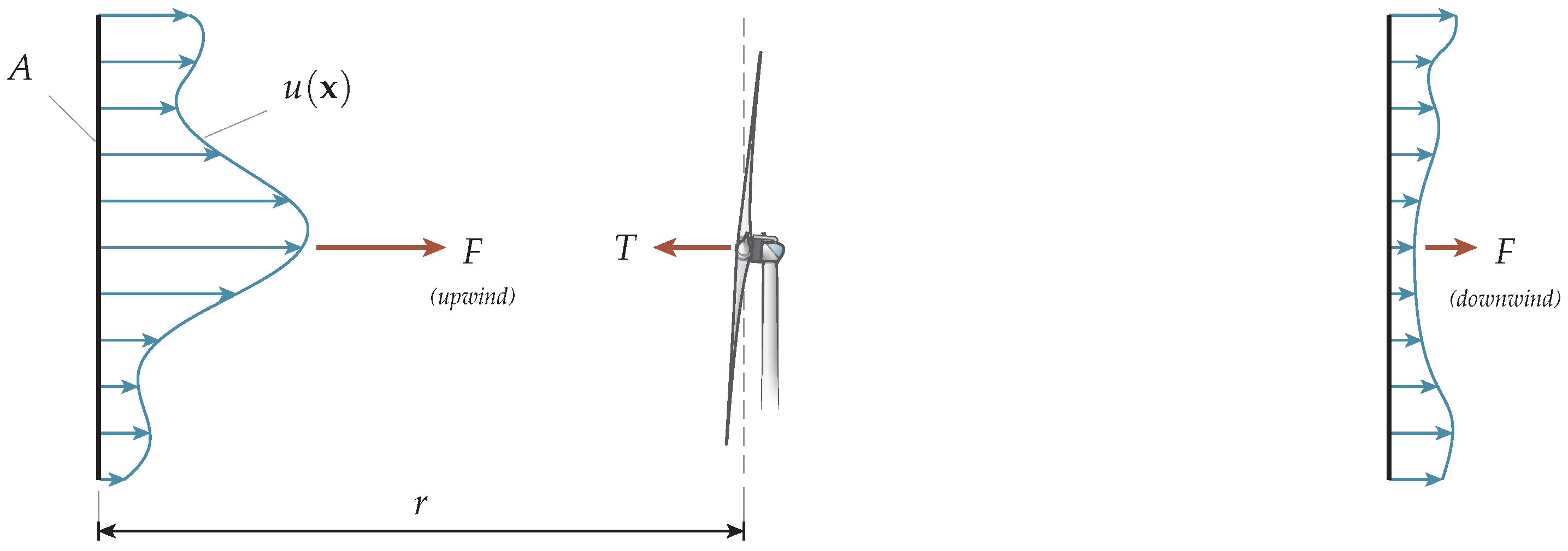
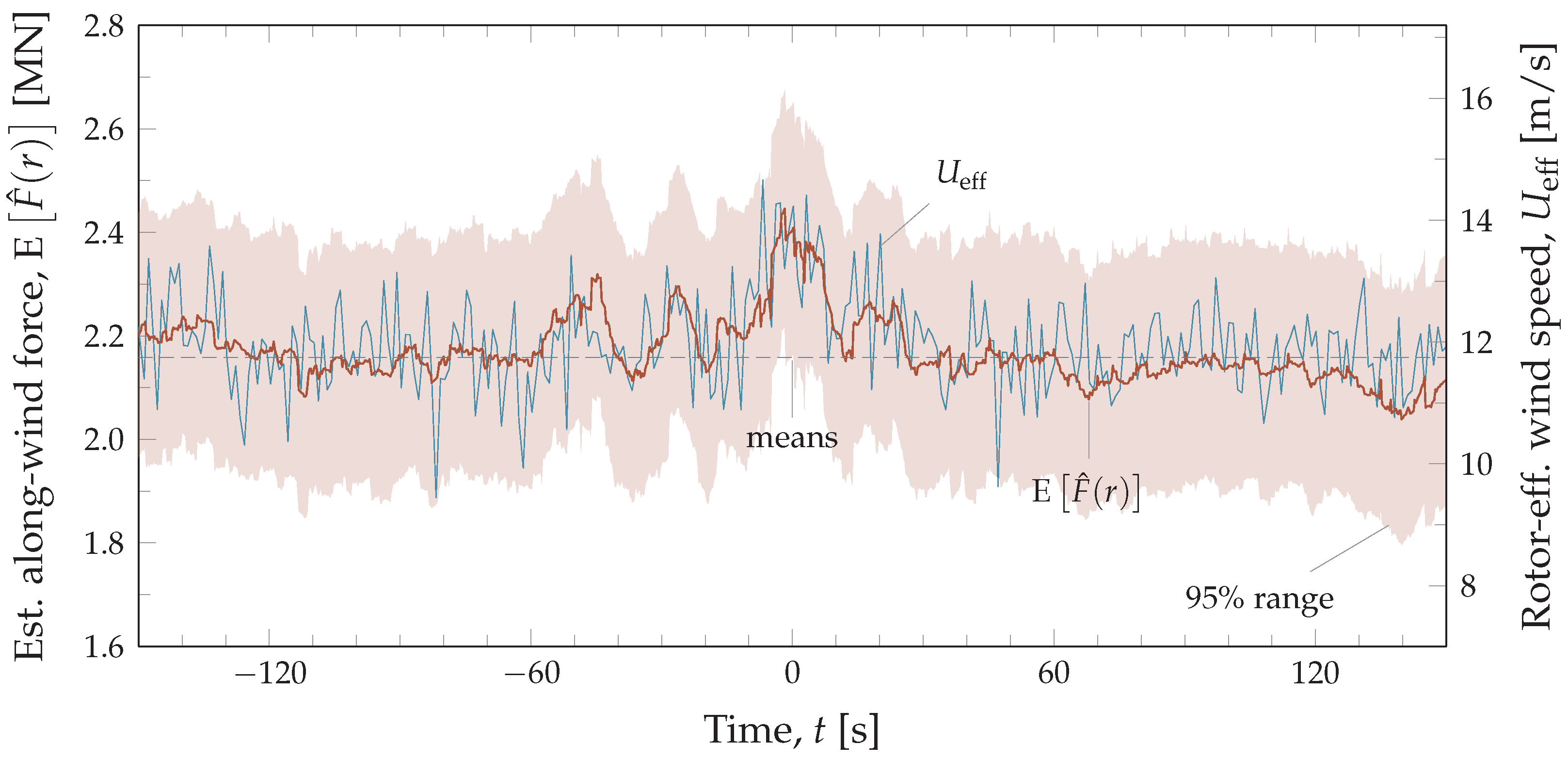
As a validation check, the expected along-wind force, E F ^ , is compared to the rotor-effective wind speed, which is a pseudo signal derived from the shaft torque, Q, and should be representative of the loads. Using this as an input for feed-forward control has shown to improve the turbine behavior in the case of severe wind gusts [13,23] and has been used extensively by ECN for research and operation. The rotor-effective wind speed, U eff , follows from
Q = 1 16 ρ C Q ( θ , λ ) π D 3 U eff 2 ,
where D is the rotor diameter and C Q is a dimensionless torque coefficient that depends on the blade pitch angle, θ, and tip speed ratio, λ. A comparison of U eff with the predicted along-wind force, shown in Figure 7, confirms that the method is able to capture the most important trends well (i.e., the low-frequency up- and downcrossings). The signals cannot be expected to match perfectly, however, since U eff is affected by any actions taken by the controller and also contains a lot of high-frequency noise coming from structural vibrations.

4. Discussion

The expected along-wind force at a certain upwind distance, E F ^ ( r ) , together with its variance, is a single signal that can be easily compared to some threshold value, making it possible to devise a control strategy based on avoiding risk. For example, if a designer accepts a 0.1% probability of F exceeding 3.0 MN, the controller would need to take action if E F ^ ( r ) + 3 σ F > 3 . 0 MN. Avoiding high loads is then done by collectively pitching the blades to decrease the rotor thrust. Modern-day multi-megawatt turbines can pitch at a rate of ± 10 deg/s, which should be fast enough to handle a gust measured 140 m upwind (especially when considering that the highest loads are generally found around rated wind speeds in the order of 10–12 m/s). Distilling the lidar measurements into a single force also helps to put individual velocity peaks into perspective. This is needed to avoid unnecessary control actions that could lead to power fluctuations, additional loading, and wear in the actuators. Alternatively, if the integral in Equation (27) is carried out per rotor annulus, it could provide a set of signals to a smart rotor (i.e., a machine with flaps distributed along its blades).
How well the statistics of F match with reality will depend on how close u ( x ) is to a stationary homogeneous Gaussian velocity field. Stationarity will not be the case during a storm or at the outflow boundary of a downdraft. Homogeneity is usually a questionable assumption for large vertical separations or under stable conditions. For example, the velocity variances, σ u 2 , σ v 2 , and σ w 2 , usually decrease with height [24]. This would mean that the severity of gusts will likely be underpredicted in the bottom half of the rotor plane (where the turbulence intensity is actually higher than what is predicted at hub height) and overpredicted in the upper half. Due to the shape of the variance profile, this will likely lead to a conservative estimate for F. It is possible to use an alternative shape of the spectral tensor to account for the vertical inhomogeneity (e.g., Φ ( κ x , κ y , z ) ), but that requires more information of the flow than lidars currently can provide. Furthermore, Gaussianity is a property that is violated on a smaller scale [25]. However, this should not have a major impact on the quality of the forecast, since most of the momentum is carried by the large-scale flow structures. In any case, some future work will have to be done on validating the correlation of the predicted along-wind force with the loads acting on the turbine, preferably using longer time series.
One of the strengths of this method is the ability to deal with missing measurements. This is needed when the lidar is mounted on the top of the nacelle with blades passing in front of the lens. Any serious gaps in the data will raise the uncertainty and therefore the risk associated with an oncoming gust, which can be included in the control strategy. In addition, since the method can handle any set of scattered velocity measurements, it should be compatible with any scanning pattern the lidar might have (e.g., see [26]).
A final remark has to be made on the evolution of wind traveling towards the turbine. Depending on the mean wind speed and which slice of the flow field is used to derive the along-wind force, the lidar can grant somewhere between 5 and 30 s of look-ahead time. During this time, the wind field would have inevitably changed. The statistics of such an evolving wind field are perhaps best predicted by considering the evolution of the Fourier modes, yielding an expression in the shape of
n ^ ( t ) = f t ; n ( t 0 ) ,
where the Fourier modes are a function of time and an initial state at a time t 0 . For example, the effect of the diffusion on the total uncertainty can be modeled by a wave number-dependent decay function where the state of the field slowly decorrelates from an initial state (e.g., see [27]). In addition, there is the effect of the induction field in front of the turbine. As the flow expands, the wave numbers are stretched and the variances of the velocity components will change. Such effects could be included in the spectral tensor, most notably in its decomposition matrix, C , with a linear transformation:
C ( κ ( t ) ) = T t 0 t C ( κ ( t 0 ) ) .
This would lead to solutions similar to those resulting from rapid distortion theory (e.g., see [17,28]), used to predict the properties of turbulence after moving through wind tunnel contractions. However, this would require some more validation and will be the subject of future study.

5. Conclusions

The goal of this paper was to present a method to turn lidar measurements of an oncoming gust into useful control input. This method works by fitting a homogeneous Gaussian velocity field to a set of scattered measurement points. From this field, an along-wind force can be derived by integrating the dynamic pressure over the rotor plane, which acts as a measure for the damaging potential of an upwind velocity peak.
The assumption of a homogeneous Gaussian velocity field allows one to analytically compute the uncertainty associated with some inherent weaknesses of the lidar system (i.e., range weighting, cyclops dilemma, and missing measurements). These uncertainties can then be included in the prediction of the along-wind force. A controller can use this to make a probablistic forecast of an oncoming gust and take preventive action based on avoiding risk.
A real-life example of the method illustrated that this is able to put individual velocity peaks, measured by several lidar beams, into perspective by computing their contribution to the total along-wind force. Furthermore, the important low-frequency up- and downcrossings found in the predicted along-wind force agree with those found in the rotor-effective wind speed employed by Van der Hooft [23]. This rotor-effective wind speed has been proven to improve turbine performance under gust loading when used as an input for feed-forward control.

Acknowledgments

This work was carried out in the scope of the INNWIND.EU project, supported by the EU FP7 programme, and the LAWINE project (Lidar Applications for Wind farm Efficiency), supported by TKI Wind op Zee. The open-access publishing fee is covered by the library of the Delft University of Technology.

Author Contributions

R. Bos devised the method and wrote the paper. A. Giyanani performed the data analysis. W. Bierbooms reviewed and edited the paper.

Conflicts of Interest

The authors declare no conflict of interest.

References

  1. Harris, M.; Hand, M.; Wright, A. Lidar for Turbine Control; Technical Report NREL/TP-500-39154; National Renewable Energy Laboratory: Golden, CO, USA, 2006.
  2. Dunne, F.; Simley, E.; Pao, L.Y. LIDAR Wind Speed Measurement Analysis and Feed-Forward Blade Pitch Control for Load Mitigation in Wind Turbines; Technical Report NREL/SR-5000-52098; National Renewable Energy Laboratory: Golden, CO, USA, 2011.
  3. Bossanyi, E.A.; Kumar, A.; Hugues-Salas, O. Wind turbine control applications of turbine-mounted LIDAR. J. Phys. Conf. Ser. 2014, 555. [Google Scholar] [CrossRef]
  4. Fürst, H.; Schlipf, D.; Latour, M.I.; Cheng, P.-W. Design and evaluation of a lidar-based feedforward controller for the INNWIND.EU 10 MW wind turbine. In Proceedings of the EWEA Annual Event, Paris, France, 17–20 November 2015.
  5. Schlipf, D.; Schlipf, D.J.; Kühn, M. Nonlinear model predictive control of wind turbines using LIDAR. Wind Energy 2013, 16, 1107–1129. [Google Scholar] [CrossRef]
  6. International Electrotechnical Commission (IEC). 61400-1 Wind Turbines—Part 1: Design Requirements, 3rd ed.; IEC: Geneva, Switzerland, 2005. [Google Scholar]
  7. Schlipf, D.; Kapp, S.; Anger, J.; Bischoff, O.; Hofsäß, M.; Rettenmeier, A.; Kühn, M. Prospects of optimization of energy production by LiDAR assisted control of wind turbines. In Proceedings of the EWEA Annual Event, Brussels, Belgium, 14–17 March 2011.
  8. Sathe, A.; Mann, J.; Gottschall, J.; Courtney, M.S. Can wind lidars measure turbulence? J. Atmos. Ocean. Technol. 2011, 28, 853–868. [Google Scholar] [CrossRef]
  9. Branlard, E.; Pedersen, A.T.; Mann, J.; Angelou, N.; Fischer, A.; Mikkelsen, T.; Harris, M.; Slinger, C.; Montes, B.F. Retrieving wind statistics from average spectrum of continuous-wave lidar. Atmos. Meas. Tech. 2013, 6, 1673–1683. [Google Scholar] [CrossRef] [Green Version]
  10. Mikkelsen, T.; Angelou, N.; Hansen, K.; Sjöholm, M.; Harris, M.; Slinger, C.; Hadley, P.; Scullion, R.; Ellis, G.; Vives, G. A spinner-integrated wind lidar for enhanced wind turbine control. Wind Energy 2013, 16, 625–643. [Google Scholar] [CrossRef] [Green Version]
  11. Kapp, S.; Kühn, M. A five-parameter wind field estimation method based on spherical upwind LiDAR measurements. J. Phys. Conf. Ser. 2014, 555. [Google Scholar] [CrossRef]
  12. Towers, P.; Jones, B.L. Real-time wind field reconstruction from LiDAR measurements using a dynamic wind model and state estimation. Wind Energy 2016, 19, 133–150. [Google Scholar] [CrossRef]
  13. Van der Hooft, E.L.; van Engelen, T.G. Estimated wind speed feed forward control. In Proceedings of the European Wind Energy Conference, London, UK, 22–25 November 2004.
  14. Schlipf, D.; Cheng, P.-W.; Mann, J. Model of the correlation between lidar systems and wind turbines for lidar-assisted control. J. Atmos. Ocean. Technol. 2013, 30, 2233–2240. [Google Scholar] [CrossRef]
  15. Simley, E.; Pao, L.Y.; Frehlich, R.; Jonkman, B.; Kelley, N. Analysis of light detection and ranging wind speed measurements for wind turbine control. Wind Energy 2014, 17, 413–433. [Google Scholar] [CrossRef]
  16. Frehlich, R.; Meillier, Y.; Jensen, M.L.; Balsley, B.; Sharman, R. Measurements of boundary layer profiles in an urban environment. J. Appl. Meteorol. Climatol. 2006, 45, 821–837. [Google Scholar] [CrossRef]
  17. Batchelor, G.K. The Theory of Homogeneous Turbulence; Cambridge University Press: Cambridge, UK, 1953. [Google Scholar]
  18. Wilson, D.K. Turbulence Models and the Synthesis of Random Fields for Acoustic Wave Propagation Calculations; Army Research Laboratory: Adelphi, MD, USA, 1998. [Google Scholar]
  19. Schlipf, D.; Trabucchi, D.; Bischoff, O.; Hofsäss, M.; Mann, J.; Mikkelsen, T.; Rettenmeier, A.; Trujillo, J.; Kühn, M. Testing of frozen turbulence hypothesis for wind turbine applications with a scanning LiDAR system. In Proceedings of the 15th International Symposium for the Advancement of Boundary Layer Remote Sensing, Paris, France, 28–30 June 2010.
  20. De Jong, J.J.M.; de Vries, A.C.; Klaasen, W. Influence of obstacles on the aerodynamic roughness of the Netherlands. Bound Lay. Meteorol. 1990, 91, 51–64. [Google Scholar] [CrossRef]
  21. Mann, J. The spatial structure of neutral atmospheric surface-layer turbulence. J. Fluid Mech. 1994, 273, 141–168. [Google Scholar] [CrossRef]
  22. Sathe, A.R.; Mann, J.; Barlas, T.; Bierbooms, W.A.A.M.; van Bussel, G.J.W. Influence of atmospheric stability on wind turbine loads. Wind Energy 2013, 16, 1013–1032. [Google Scholar] [CrossRef]
  23. Van der Hooft, E.L.; Schaak, P.; van Engelen, T.G. Wind Turbine Control Algorithms; Energy Research Centre of The Netherlands: Petten, The Netherlands, 2003. [Google Scholar]
  24. Suomi, I.; Gryning, S.-E.; Floors, R.R.; Vihma, T.; Fortelius, C. On the vertical structure of wind gusts. Q. J. R. Meteorol. Soc. 2015, 141, 1658–1670. [Google Scholar] [CrossRef]
  25. Castaing, B.; Gagne, Y.; Hopfinger, E.J. Velocity probability density functions of high Reynolds number turbulence. Physica D 1990, 46, 177–200. [Google Scholar] [CrossRef]
  26. Dimitrov, N.; Natarajan, A. Application of simulated lidar scanning patterns to constrained Gaussian turbulence fields for load validation. Wind Energy 2016. [Google Scholar] [CrossRef]
  27. Bossanyi, E. Un-freezing the turbulence: Application to LiDAR-assisted wind turbine control. IET Renew. Power Gener. 2013, 7, 321–329. [Google Scholar] [CrossRef]
  28. Townsend, A.A. The response of sheared turbulence to additional distortion. J. Fluid Mech. 1980, 98, 171–191. [Google Scholar] [CrossRef]
Figure 1. Drawing of the pulsed lidar system, mounted on the nacelle of a Darwind XD115-5MW wind turbine.
Remotesensing 08 00758 g001
Figure 2. A collection of line-of-sight velocities measured within a certain time period. The distance between the range gates is Δ R = 15 m. Every time step, the points advect downstream with a mean velocity u ¯ ( x j ) .
Remotesensing 08 00758 g002
Figure 3. The along-wind force, F, is a good measure for the risk associated with an upcoming gust. The thrust force, T, which dictates the loads acting on the structure, is a result of momentum transfer between the wind and the rotor and is difficult to predict in advance. However, the severitiy (i.e., the damaging potential) of a gust, is captured by the upwind F.
Remotesensing 08 00758 g003
Figure 4. Longitudinal velocity spectrum, taken as the average of 12 ten-minute spectra measured along the center beam over the 2 h period preceding the gust event. During this period, the conditions were comparable ( 12 . 5 u ¯ 16 . 0 m/s) and the wind direction was relatively constant ( ± 5 ).
Remotesensing 08 00758 g004
Figure 5. Streamwise velocity fields based on one full cycle of measurements ( n = 50 ). The dots pinpoint the locations of the individual points, including the distance they are expected to have advected within the 1.25 s measurement period (see Figure 2). (a) the expectation of u ^ ( r , y , z ) (i.e., in the y z -plane at r = 140 m); (b) the expectation of u ^ ( x , 0 , z ) ; (c) the variance of u ^ ( r , y , z ) with respect to the longitudinal variance, σ u 2 ; and (d) the variance of u ^ ( x , 0 , z ) with respect to the longitudinal variance, σ u 2 .
Remotesensing 08 00758 g005
Figure 6. Construction of an estimated along-wind force, F ^ (a), and its variance (b), from five individual velocity signals, u 0 , , u 4 (cg) at the r = 140 m range gate (where 0–4 are the beam positions). The time series are centered around a gust event at t = 0 .
Remotesensing 08 00758 g006aRemotesensing 08 00758 g006b
Figure 7. Comparison of the along-wind force forecasted with lidar (including a 10.5 s delay to account for steady advection from r = 140 m to r = 0 m with u ¯ = 13 . 3 m/s) and the rotor-effective wind speed derived from the turbine shaft torque (downsampled to 1 Hz for clarity).
Remotesensing 08 00758 g007

