Gap-Filling of Landsat 7 Imagery Using the Direct Sampling Method

Abstract

The failure of the Scan Line Corrector (SLC) on Landsat 7 imposed systematic data gaps on retrieved imagery and removed the capacity to provide spatially continuous fields. While a number of methods have been developed to fill these gaps, most of the proposed techniques are only applicable over relatively homogeneous areas. When they are applied to heterogeneous landscapes, retrieving image features and elements can become challenging. Here we present a gap-filling approach that is based on the adoption of the Direct Sampling multiple-point geostatistical method. The method employs a conditional stochastic resampling of known areas in a training image to simulate unknown locations. The approach is assessed across a range of both homogeneous and heterogeneous regions. Simulation results show that for homogeneous areas, satisfactory results can be obtained by simply adopting non-gap locations in the target image as baseline training data. For heterogeneous landscapes, bivariate simulations using an auxiliary variable acquired at a different date provides more accurate results than univariate simulations, especially as land cover complexity increases. Apart from recovering spatially continuous fields, one of the key advantages of the Direct Sampling is the relatively straightforward implementation process that relies on relatively few parameters.

1. Introduction

The Landsat 7 satellite was launched in April, 1999 with an aim of providing timely and high quality visible and infrared images of the Earth’s surface, while fulfilling the goal of mission data continuity that had been established from preceding platforms [1]. One of the principal objectives of the Landsat Program, a joint effort of the U.S. Geological Survey (USGS) and the National Aeronautics and Space Administration (NASA), was to develop a long-term and spatially consistent record of natural and human-induced changes on the global landscape [2]. The Landsat program has been successful in this task and has played a foundational role across a diverse range of studies with focus areas in agriculture, forestry, water quality and geology, to name just a few.

Unfortunately, the Scan Line Corrector (SLC; an electromechanical device that compensates for the forward motion of the satellite) on Landsat 7’s Enhanced Thematic Mapper Plus (ETM+) instrument, failed on 31 May 2003. Consequently, the once spatially continuous fields observed from the sensor were affected by a line-of-sight zig-zag pattern, resulting in large gaps and around 22% of pixels missing in collected data. While still providing usable and accurate data, the utility of the observations was significantly impaired. In order to assess the scale of the SLC problem, scientists were gathered to evaluate the utility and validity of Landsat 7 products after the SLC failure [3]. Overall, it was found that for those applications operating at large spatial scales, such as land cover change and qualitative assessments of crops, the effect of the anomaly was slight or tolerable, while for applications requiring complete and focused retrievals over localized areas, such as detailed mapping or event monitoring, the anomaly could not be ignored [3]. Ultimately, finding a method to satisfactorily fill the gaps was necessary.

To address this task, a variety of techniques have been proposed, with the Local Linear Histogram Matching (LLHM) approach [4,5] being one of the first considered by the USGS. In this approach (and in subsequent examples used herein), the image containing gaps is referred to as the target image, while the images that provide information to fill these gaps are referred to as input images. The LLHM method uses a geometrically consistent Landsat 7 image collected prior to the anomaly as an input image and attempts to find the linear transformation of the digital number (DN) of the non-gap locations between the input image and target image. While the method is conceptually simple, the results are in general only passable. Some striping appears around land cover changes, and artifacts occur around small sharp edges, which generally limits the usage of LLHM to homogeneous land types. To address the limitations inherent in the LLHM method, Maxwell et al. [6] introduced an approach to fill the gaps based on a multi-scale segment model. The idea of segmentation is to group individual pixels into a series of size groups (scale 10, 15 and 20 were used in Maxwell et al. 2007) according to their spectral and spatial characteristics [7]. However, like the LLHM, the approach is most suited to homogeneous areas, as it is not able to depict the characteristics of more heterogeneous landscapes. Pringle et al. [8] proposed geostatistical interpolation to fill the gaps, recommending the co-kriging algorithm to predict the missing values [9,10]. Two cloud-free input images are used, with one taken earlier and another after the target image. Ideally, the two input images should be temporally close to the target image. However, the utility of this approach is reduced as the availability of temporally close gap-free imagery becomes limited. Further, the implementation of geostatistical approaches is generally based on the assumption of a stationary spatial process, which is not plausible when land cover is expected to change dynamically in both space and time.

In more recent work, Chen et al. [11] proposed a deterministic approach, referred to as the Neighborhood Similar Pixel Interpolator (NSPI), to improve the performance of predicting heterogeneous areas. The NSPI assumes that neighborhood pixels close to the un-scanned (i.e., gap) pixel share similar spectral characteristics and temporal patterns of changes to the un-scanned pixel(s). By combining the information provided by the neighborhood pixels, the value of the missing pixels can be determined. Results have shown that the NSPI produces far better continuous characteristics compared with previous methods. However, one issue requiring consideration is that the NSPI is a deterministic approach. Indeed, the question of how input images affect the fidelity of the final simulation results remains unknown, which may weaken the reliability of the simulation results significantly. To address this problem, Zhu et al. [12] introduced the Geostatistical Neighborhood Similar Pixel Interpolation (GNSPI), which improved NSPI by combining geostatistical theory and demonstrated a more accurate result when compared to the NSPI alone. GNSPI divides the reflectance value of an un-scanned pixel into a temporal trend and residual, of which the temporal trend is estimated based on NSPI and the residual is predicted through an ordinary kriging algorithm. Although the simulation results from the GNSPI make it one of the best performing methods to date, its relatively complicated operation as well as computational constraints limits its application. Zeng et al. [13] proposed a weighted linear regression (WLR) algorithm integrated with Laplacian prior regularization to recover missing pixels in SLC-off imagery. The WLR algorithm builds a linear regression model between the corresponding pixels of multi-temporal images to fill the majority of missing pixels. The Laplacian prior regularization method, a non-reference regularization method, is then applied to fill those gap pixels that cannot be completely recovered by WLR algorithm. The integrated approach has been demonstrated to reconstruct complicated landscapes accurately. However, its performance becomes limited when applied to complex landscapes with large data gaps.

Multiple-point geostatistics (MPS) [14,15] is a modeling approach that uses training images to develop stochastic representations of spatial phenomena. The idea behind multiple-point geostatistics is to infer the multiple-point conditional distribution directly from selected training images and then reconstruct complicated structures using the patterns present in given training images. The sources of training imagery are various and can include, for instance, remotely sensed images, experimental data or modeling results. One important concept in the MPS approach is the data event, which is the pattern of values consisting of the n closest neighborhood pixels of the unknown pixel x in the target image. One early algorithm for MPS is the method proposed by Guardiano and Srivastava [14]. In this approach, the entire training image is scanned and all training replicates that perfectly match the data event (i.e., training replicates have the same values as the data event at corresponding locations) are found and stored. Based on this matching set, the conditional cumulative distribution function (ccdf) of x can be determined and a sample is then randomly drawn from this distribution to fill unknown pixels.

One problem impeding the practical application of this algorithm is that it requires a scan of the entire training image to predict the value of each single pixel, which is clearly time-consuming. Strebelle improved the applicability of MPS by introducing the Single Normal Equation Simulation (SNESIM) algorithm [16], which includes a search tree structure where training replicates of all data events are recorded and stored, making MPS more practical. Considering the difficulty of deriving the ccdf from a continuous TI, the SNESIM algorithm can only be applied to categorical variables. A number of alternative methods including the SIMPAT algorithm [17], unilateral path algorithm [18] and FILTERSIM algorithm [19], have also been proposed to deal with both categorical and continuous variables. To date, MPS has been widely used for the reconstruction of complex geological structures [20,21,22] and in more recent years, has been applied to analyze remote sensing land cover classification [23,24] as well as downscaling applications [25,26]. As such, the method is anticipated to serve as an efficient approach to fill gaps within remote sensing imagery, caused for instance by cloud cover and orbital characteristics [27] or, as in the case to be explored here, instrument failure.

To advance the application of MPS approaches for gap-filling efforts, we explore the use of the Direct Sampling method as proposed in Mariethoz et al. [28]. The Direct Sampling method uses a conditional stochastic resampling of known areas in the training image to simulate the unknown locations in the target image and allows for the generation of multiple and equiprobable stochastic reconstructions. The applicability of Direct Sampling has been demonstrated previously across a range of applications, which include the downscaling of climate simulations [29] as well as the simulation of daily rainfall time series [30]. To evaluate the gap-filling potential of Direct Sampling more thoroughly, the approach will be assessed against Landsat data covering a range of challenging land cover types, including deserts, sparse agricultural areas, dense farmlands and urban areas, as well as braided rivers and coastal area. To examine the impact of temporal distance on the fidelity of the simulation results, for each studied land cover type, a series of input images at approximately two weeks, four weeks, six weeks and longer than four months separation from the target image are used to provide gap-filling information. The influence of the choice of input imagery on prediction accuracy is also considered. The reconstruction results are examined using both quantitative and qualitative descriptors to identify the utility of the Direct Sampling method.

2. Materials and Methods

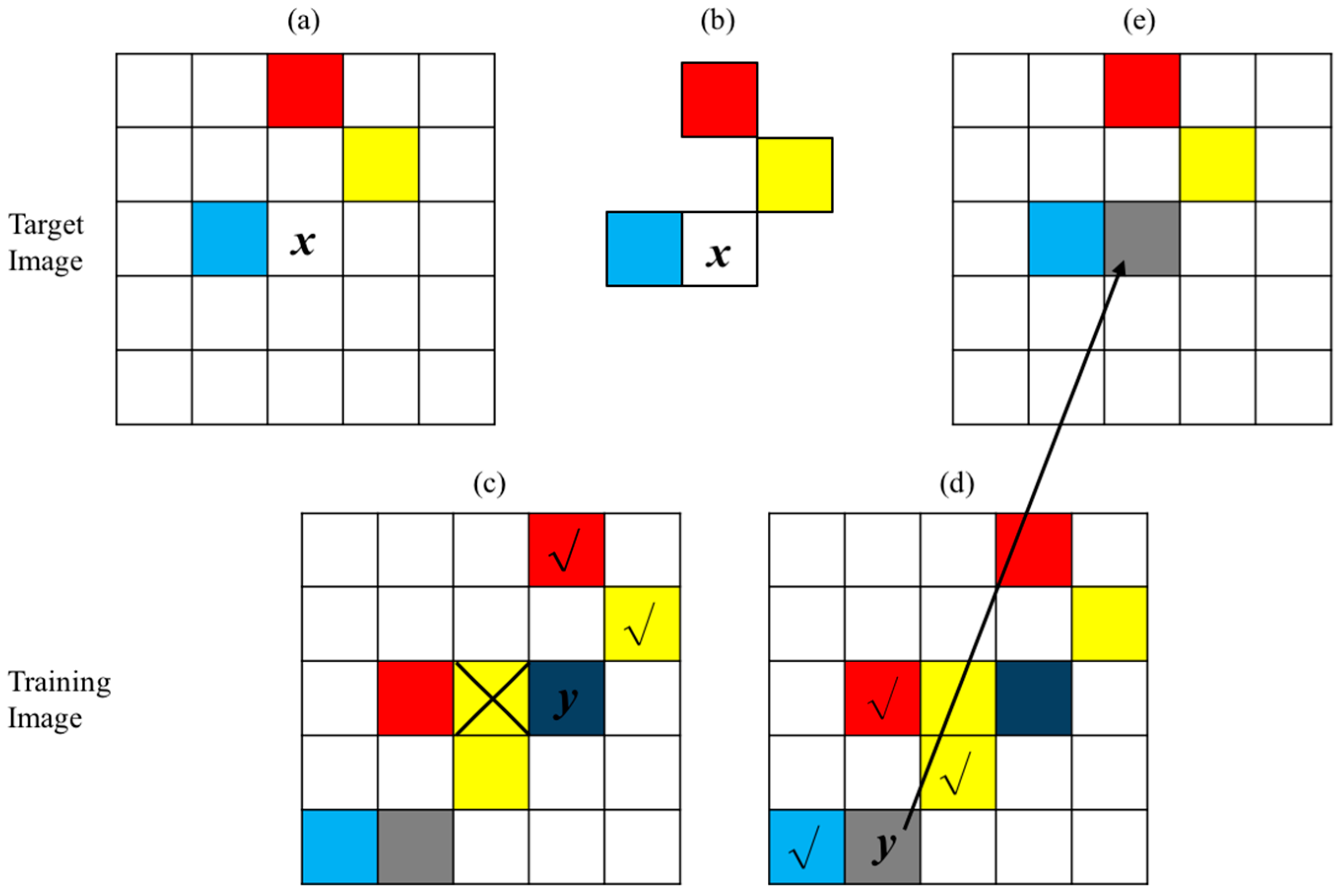
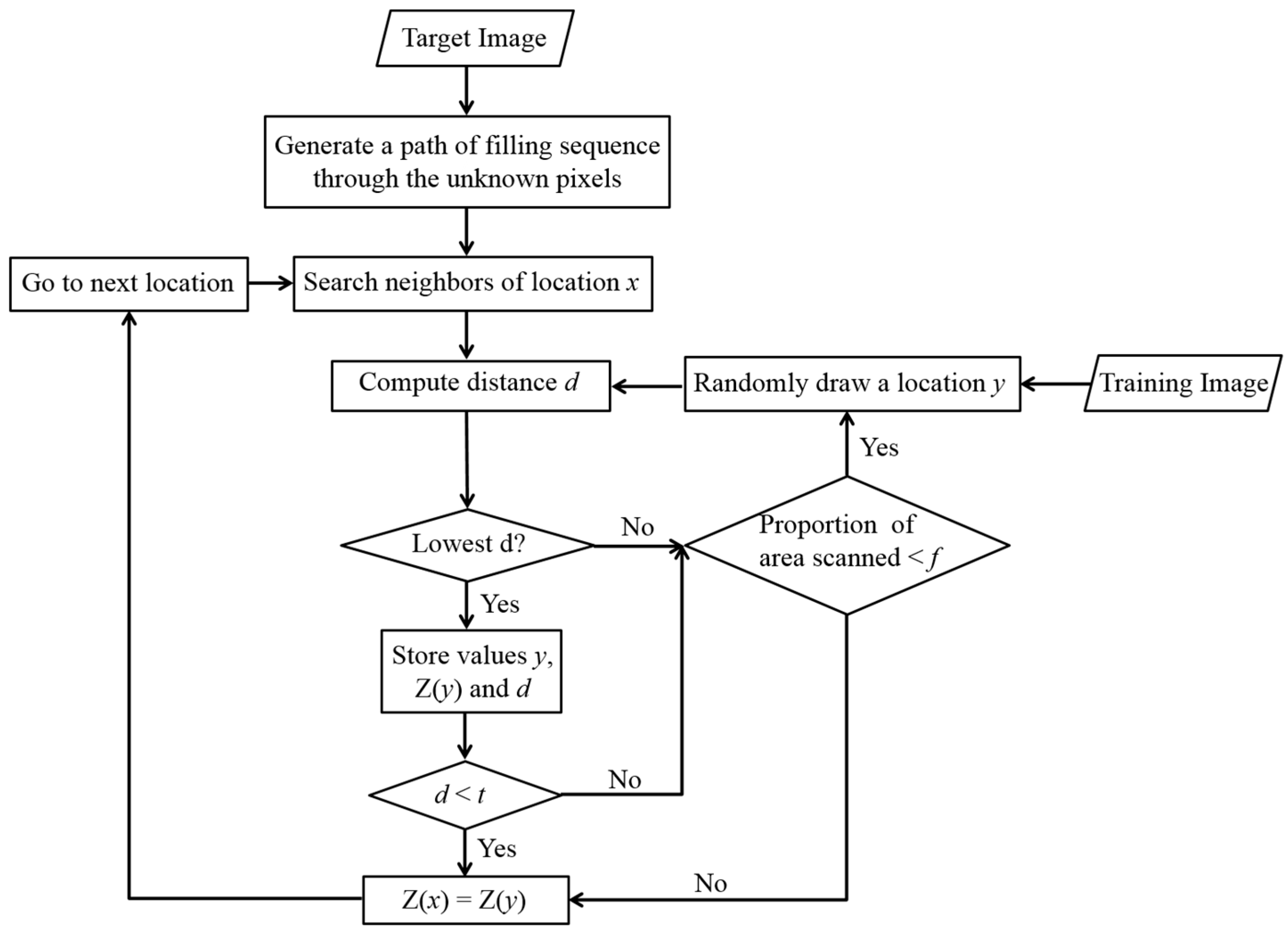
2.1. Direct Sampling Method

The Direct Sampling method adopted in this paper generates stochastic fields that present complex statistical and spatial properties based on training images [27]. The particular features of the Direct Sampling method compared to other MPS algorithms is that it does not demand an explicit computation and storage of the ccdf expressed in Equation (1):

$$F\left(z,x,N_x\right)=Prob(Z\left(x\right)\le \mathrm{z}|N_x)$$

(1)

where Z(x) is the variable of interest, x is the location of an unknown pixel and N_x is the data event consisting of the pattern of values made by the n closest neighbors of x: {x₁, x₂,…, x_n}. For each unknown pixel x, N_x is made of the values of Z at the neighboring locations, {Z(x₁), Z(x₂), …, Z(x_n)}, as well as the lag vectors that describe the relative positions between location x and its neighborhoods, defined as L = {h₁, h₂, …, h_n} = {x₁ − x, x₂ − x, …, x_n − x}. The Direct Sampling method acquires the values of unknown pixels Z(x) by directly sampling the training image in a random manner, attempting to find one pixel y in the training image with a replicate N_y that is similar to N_x [31]. As soon as a pixel y is obtained with a neighborhood similar to N_x, the sampling process stops and the value of y is assigned to x.

To clarify the process of the Direct Sampling method, the gap-filling procedure of a categorical variable is displayed in Figure 1. In this example, Figure 1a is the target image with unknown pixels to be filled, of which white pixels are unknown and colored pixels are informed. The filling path of all un-scanned pixels is generated randomly. The pixel denoted by a question mark is the target pixel x to be predicted at the current step and the data event N_x is defined in (b). Figure 1c is a training image used to fill the target pixels. The data event (b) is used to search the training image randomly. The search process continues until one replicate N_y that can exactly match the defined data event N_x is found in the training image. Once the matched replicate N_y is found (Figure 1d, check marks), the search process stops and the value of y is assigned to the target pixel x, as shown in Figure 1e. The new pixel value is then considered known and the procedure (a)–(d) is repeated to simulate the value of another unknown pixel. Each time, the previously simulated pixels are considered in subsequent data events. The order in which pixels are simulated is defined by a random path which is different for each realization.

The gap-filling procedure for a continuous variable (Figure 2) is slightly different from the categorical variables as it is unrealistic to find a replicate in the training image which is completely the same as the defined data event. A distance criterion is introduced with the notation d(N_x, N_y) to choose the replicates for filling gap pixels. The distance is a metric used to assess the similarity between the replicate N_y found in the training image and the data event N_x. When the distance is less than a given threshold t, N_y is regarded similar as N_x and the value of y is assigned to x. The distance can be computed in different ways (further discussion on this can be found in Mariethoz et al. [31]).

In this paper, the Landsat reflectance data is a continuous variable, hence the Euclidian Distance is favored, expressed in Equation (2) as:

$$d(N_x,N_y)=\frac{1}{\eta }\sqrt{{\displaystyle \sum }_{i=1}^n{\left[Z(x_i-Z\left(y_i\right)\right]}^2}$$

(2)

where ƞ is a normalization factor defined as the difference between the maximum and minimum values in the training image and ensures that the distance remains bounded within the interval [0,1]. The threshold t is also defined in the same interval, of which t = 0 reflects the highest accuracy allowing no discrepancy in the simulated patterns and t = 1 assumes complete data event mismatch. Usually, it is impossible to achieve a 0 threshold, so a very small t value is set. For each step of searching replicates, the replicate giving the lowest distance will be stored until one replicate that gives a distance lower than the threshold is found. To balance the prediction accuracy and computational time, a fraction parameter f is introduced. Fraction is the maximum proportion of the training image to be searched for each target pixel. When the search proportion of the training image exceeds a fraction f without replicates fulfilling the threshold requirement found, the value of the pixel y with the lowest distance will be assigned to Z(x). The concept of Direct Sampling is relatively simple, with only three main parameters comprising the number of neighbors n, threshold t and fraction f, to be considered in generating the simulation. Since the Direct Sampling is a stochastic method, multiple equiprobable reconstructions can be generated to quantify uncertainty.

In this study, the Direct Sampling fills missing pixels by deriving values from portions of the training image that satisfy a distance to a data event that is less than the specified threshold t, with the training image covering the same area as the target image (but from a different date). In cases where a significant portion of the target image is already known, the Direct Sampling can work without using any additional training imagery, with the non-gap locations in the target image functioning as the training data to fill the gaps. In addition to these so called univariate cases, the Direct Sampling can also be applied to multivariate simulations, with the process conceptually similar to the univariate simulation, but with the difference being in the selection of neighborhood pixels and the definition of distance. Figure 3 illustrates the selection of neighborhood pixels in multivariate simulations (bivariate simulations examined in this study). Figure 3a shows the target images, with the values of observed pixels (i.e., colored pixels) different for the two variables. Figure 3b displays the training images with the same two variables. The pixel with a red question mark in Figure 3a is the target pixel x to be predicted at the current step, and its closest seven pixels are selected as neighborhood pixels. Neighborhoods are defined on both variables. One replicate N_y found in the training image is shown in Figure 3b with pixels marked in red. The distance is computed by calculating a weighted average of the univariate distance of each variable, as shown in Equation (3):

$$d\left(N_x^{\prime },N_y^{\prime }\right)={\displaystyle \sum }_{\kappa =1}^m\frac{{\alpha }_{\kappa }}{{\eta }_{\kappa }}\sqrt{{\displaystyle \sum }_{i=1}^{\mathrm{n}}{\left[Z^{\kappa }\left(x_i\right)-Z^{\kappa }\left(y_i\right)\right]}^2}$$

(3)

where m is the number of variables, α_k are weight given to each variable summing to 1, and ƞ_k is the normalization constant for each variable.

Both univariate and bivariate cases are explored in this study. A more detailed description of the implementation details and a practical guide for the use of the Direct Sampling can be found in Mariethoz et al. [28] and Meerschman et al. [32].

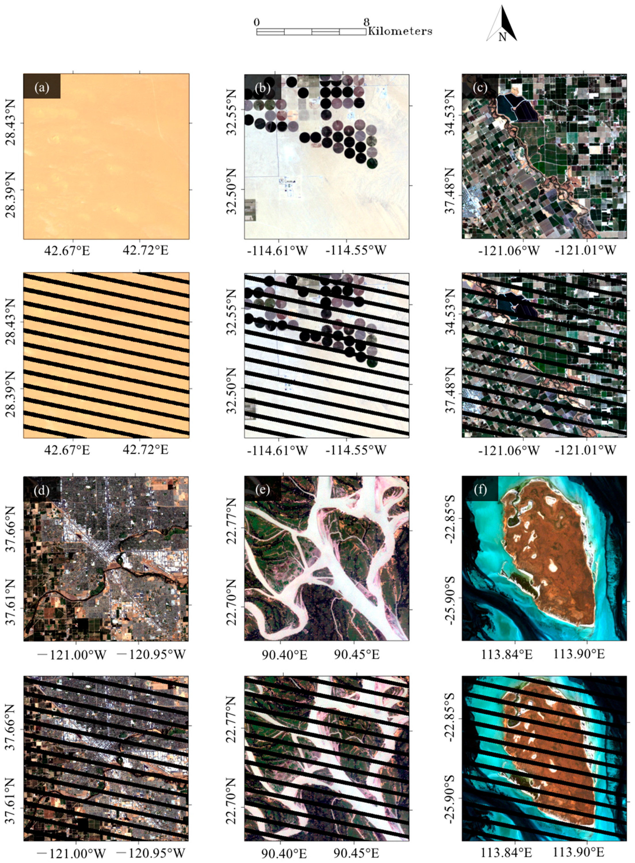
2.2. Experiment Design

To examine the impacts of varying influence of land surface heterogeneity on the gap-filling procedure, six regions dominated by different land cover types are used, comprising desert (R1), sparse agricultural (R2), dense farmland (R3), urban (R4), braided river (R5) and coastal (R6). All of the imagery is derived from ETM+ images, but prior to the SLC failure in order to allow for a comprehensive error characterization. Only bands 1–5 and 7 are considered here due to their similarity in spatial resolution, with band designations listed in

Table 1. Band designations of bands 1–5 and 7 of Landsat Enhanced Thematic Mapper Plus (ETM+) images.

Landsat 7	Wavelength (mm)	Resolution (m)
Band 1	0.45–0.52	30
Band 2	0.52–0.60	30
Band 3	0.63–0.69	30
Band 4	0.77–0.90	30
Band 5	1.55–1.75	30
Band 7	2.09–2.35	30

. For each of the pre-selected regions, a 400 × 400 pixel area (12 × 12 km) sub-region was extracted from the Landsat data for a more detailed assessment. The six selected sub-regions range from homogeneous to highly heterogeneous, representing an increasing spatial complexity in land cover. For heterogeneous landscapes, characteristics such as streams or small objects are deliberately included in the selected sub-regions. In addition to the land cover specific target images, four input images covering spatially coincident images, but collected over approximately two weeks, four weeks, six weeks and longer than four months temporal distance from the target images, were also selected to assess their capacity to inform the gap-filling process. In chronological order, the four input images for each land cover are defined as D1, D2, D3 and D4.

Given that the imagery was obtained prior to the SLC failure, gaps in the target images for all land covers were artificially imposed using a gap mask from an actual SLC-off ETM+ image, ensuring that the location and size of the gaps in the six target images were realistically enforced. The overpass dates of all the examined ETM+ images are listed in

Table 2. The collection dates for the target images and the four input images used for informing the gap-filling process.

	R1	R2	R3	R4	R5	R6
	Desert	Sparse Agricultural	Dense Farmland	Urban Area	Braided River	Coastal Area
Path	169	38	43	43	137	115
Row	40	37	34	34	44	78
Target image	28 August 2002	5 July 2002	8 July 2002	8 July 2002	31 October 2002	17 July 2002
Date 1	13 September 2002	19 June 2002	24 July 2002	24 July 2002	16 November 2002	1 July 2002
Date 2	29 September 2002	3 June 2002	9 August 2002	9 August 2002	2 December 2002	18 August 2002
Date 3	15 October 2002	18 May 2002	25 August 2002	25 August 2002	18 December 2002	30 May 2002
Date 4	6 April 2002	11 February 2002	2 March 2002	2 March 2002	5 March 2002	11 March 2002

. Before the gap-filling process, all input images are geometrically rectified to the target images and the digital numbers are calibrated to the top-of-atmosphere reflectance based on the method provided by the USGS [1]. Natural color images of target images are displayed in Figure 4, with the corresponding input images shown in Figure 5.

Nine individual cases including both univariate (“U-”) and bivariate (“B-”) simulations are considered for each studied region as described in

Table 3. Nine individual cases considered for each land cover type.

Case Name	Description
U-D1	Univariate case with D1 (two-week distance) as training image
U-D2	Univariate case with D2 (four-week distance) as training image
U-D3	Univariate case with D3 (six-week distance) as training image
U-D4	Univariate case with D4 (longer than four-month distance) as training image
U-D0	Univariate case with non-gap area in target image as training image. No additional image introduced
B-D1	Bivariate case, with one variable the reflectance value in the target image and another the reflectance value of D1 (two-week distance)
B-D2	Bivariate case, with one variable the reflectance value in the target image and another the reflectance value of D2 (four-week distance)
B-D3	Bivariate case, with one variable the reflectance value in the target image and another the reflectance value of D3 (six-week distance)
B-D4	Bivariate case, with one variable the reflectance value in the target image and another the reflectance value of D4 (longer than four-month distance)

. In the univariate cases, the input images are used as the training image to provide information for filling gaps. In the bivariate simulations, the input image functions as an auxiliary variable, which means that the reflectance of the input image is used in addition to the reflectance of the target image in the setting described in Figure 3. The known areas of the target image as well as the input image (both variables in Figure 3b) are used to compute the distance to the data event defined in Equation (3). When the location of a suitably similar data event y is found (i.e., with a distance below the threshold t), the corresponding value in variable 1 (the target image) is used to fill the unknown pixel x.

From Table 3, U-D1, U-D2, U-D3 and U-D4 correspond to the use of D1, D2, D3 and D4 as training images to fill the gaps in the target image respectively for the univariate case. B-D1, B-D2, B-D3 and B-D4 correspond to the usage of D1, D2, D3 and D4 as auxiliary images for the bivariate case. In the special case of U-D0, no additional input image is used, with known areas present in the target image used as the training image for the gap-filling procedure. Ten reconstruction realizations are produced for each case, with the mean realization predicted by these reconstructions used to analyze the simulation effect from both a qualitative and quantitative perspective. The selection of 10 reconstructions is a trade-off between the realization accuracy and computational time. Too few reconstructions can make the filled gaps abrupt and discontinuous, and too many may only slightly improve the prediction accuracy while increasing computational time. The parameters used in this study are the same for all cases and all land cover types, with threshold t = 0.01, fraction f = 0.75 and the number of neighbors n = 30 (see Section 2.1 and Figure 2 for a description of these parameters). Further guidance on the selection of parameters can be found in Meerschman et al. [32].

2.3. Validation of Gap-Filling Results

As the gaps are imposed manually, the original unaltered imagery can be used to evaluate the results of gap-filling. In addition to a qualitative comparison, which evaluates the ability of the Direct Sampling method to retain object shapes and continuity of features, quantitative metrics are also implemented to assess the gap-filling results. The statistical indices used here include: (1) root mean square error (RMSE); (2) mean spectral angle (MSA); (3) relative root mean square error (rRMSE); (4) coefficient of determination (R2); and (5) median absolute percentage error (MdAPE), with their definition expressed below:

• RMSE

$$\mathrm{RMSE}=\sqrt{\frac{1}{n_1}{\displaystyle \sum }_{i=1}^{n_1}{\left(Z^{*}\left(x_i,t,b\right)-Z\left(x_i,t,b\right)\right)}^2}$$

(4)

where $Z^{*}\left(x_i,t,b\right)$ is the predicted value of xi of band b at time t, and $Z\left(x_i,t,b\right)$ is the actual value of xi of band b acquired at time t. n1 is the total number of un-scanned pixels. A smaller RMSE usually represents a smaller prediction error and thus a more accurate prediction. However, the value can be significantly influenced by a few extreme prediction errors.

• MSA

$$\mathrm{MSA}=\frac{180}{\pi }\times \frac{\left({{\displaystyle \sum }}_{i=1}^{n_1}\arccos \left({{\displaystyle \sum }}_{b=1}^{n_2}{Z}^{*}\left(x_i,t,b\right)Z\left(x_i,t,b\right)/\sqrt{{{\displaystyle \sum }}_{b=1}^{n_2}{Z}^{*2}\left(x_i,t,b\right){{\displaystyle \sum }}_{b=1}^{n_2}{Z}^2\left(x_i,t,b\right)}\right)\right)}{n_1}$$

(5)

where n₂ is the number of examined bands (n₂ = 6 here), and the unit of MSA is degree (°). It is possible that one specific band can be perfectly predicted but other bands are filled with poor results, therefore MSA is used to assess the conjunct spectral fidelity of multiple bands instead of a single band. A smaller MSA generally means a more accurate prediction.

• rRMSE

$$\mathrm{rRMSE}=\sqrt{\frac{1}{n_1}{\displaystyle \sum }_{i=1}^{n_1}{\left(\frac{Z^{*}\left(x_i,t,b\right)-Z\left(x_i,t,b\right)}{Z\left(x_i,t,b\right)}\right)}^2}$$

(6)

When comparing the prediction accuracy given by the Direct Sampling method over a range of regions with different types of heterogeneity, RMSE fails to provide intercomparable results due to the reflectance value range of different regions varies. Therefore, rRMSE is adopted to calculate the relative error through a normalization technique for a direct comparison.

• R²

$$R^2={\left(\frac{{{\displaystyle \sum }}_{i=1}^{n_1}\left(Z^{*}\left(x_i,t,b\right)-\overline{Z^{*}}\left(x,t,b\right)\right)\left(Z\left(x_i,t,b\right)-\overline{Z}\left(x,t,b\right)\right)}{\sqrt{{{\displaystyle \sum }}_{i=1}^{n_1}{\left(Z^{*}\left(x_i,t,b\right)-\overline{Z^{*}}\left(x,t,b\right)\right)}^2{{\displaystyle \sum }}_{i=1}^{n_1}{\left(Z\left(x_i,t,b\right)-\overline{Z}\left(x,t,b\right)\right)}^2}}\right)}^2$$

(7)

where $\overline{Z^{*}}\left(x,t,b\right)$ and $\overline{Z}\left(x,t,b\right)$ are the mean of the predicted values and actual values. R² is an index used to describe the degree of consistency between the predicted and actual values ranging in the interval [0,1]. A value of 1 indicates that the predicted values can linearly fit the actual values perfectly, while a value of 0 means there is no linear relationship between the predicted and actual values.

• MdAPE

$$\mathrm{MdAPE}={}_{i=\overline{1,n_1}}{}^{median}\left(100\cdot \left|p_i\right|\right),p_i=\frac{\left|Z^{*}\left(x_i,t,b\right)-Z\left(x_i,t,b\right)\right|}{Z\left(x_i,t,b\right)}$$

(8)

MdAPE is the median of the relative absolute error in percentage form. As mentioned above, since the RMSE and rRMSE can be impacted by a few extreme errors, they cannot always provide effective information to assess the results of the majority of un-scanned pixels. MdAPE considers the median of the percentage error, which is more robust to extreme errors. An MdAPE value close to zero represents an unbiased prediction.

3. Results

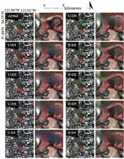
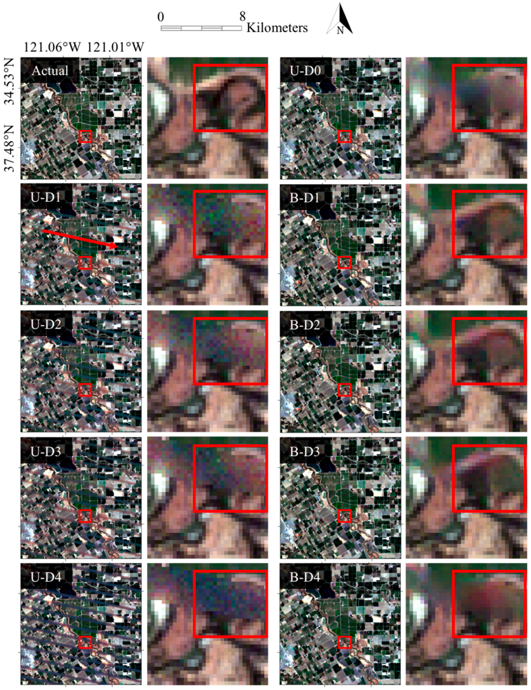
3.1. Comparison of Univariate and Bivariate Simulations

As previously mentioned, the Direct Sampling method can be implemented in both univariate and multivariate simulations. In the univariate case, the spatial features contained in the training image solely provide information for filling gaps. When bivariate simulations are conducted (i.e., the reflectance value in the target image together with reflectance value from the same area, but at a different date), both temporal and spatial features are incorporated into the simulation and are assumed to provide a more accurate result. To verify this hypothesis and explore an efficient approach for gap-filling, both univariate and bivariate simulations were examined. To simplify the presentation of results, the region dominated by dense farmland (R3) was chosen as a representative example to compare the performance of these two approaches in the discussion below.

The mean realization of 10reconstructions and the zoomed image of a small region in the mean realization for each case of the dense farmland, together with the actual images, are presented in Figure 6. Referring to cases described in Table 3, cases starting with “U-” are univariate simulations and cases starting with “B-” present bivariate simulations. D1, D2, D3 and D4 in the case names represent using input images with an increasing temporal distance of two weeks, four weeks, six weeks and longer than four months as training images in the univariate cases and auxiliary images for the bivariate cases. Recall that U-D0 is the univariate case where known areas present in the target image are used as training data for the gap-filling procedure.

As can be seen from the mean realizations, the traces of gaps (direction identified with an arrow in Figure 6 case U-D1) are discernable in all univariate simulations except for U-D0. Likewise, these traces are not observed in the realizations of the bivariate simulations. Specific image elements, such as the connectivity traits of the narrow river in the zoomed images (right hand image in each pair), cannot be adequately reproduced for all univariate simulations, although U-D0 is slightly improved related to the other univariate cases. For the bivariate cases, even though the prediction is not per-pixel accurate, the continuous stream features are relatively well preserved, with occasional discrepancies and relatively few artifacts present in the images. B-D4 provides the poorest result among all bivariate simulations, but still performs better than U-D0, which gives the most accurate results among the univariate cases. From a qualitative perspective, the conclusion that bivariate simulations produce better results compared with the univariate simulation is obvious, especially when used to fill complicated landscape elements with connectivity features. Among the univariate cases, U-D0 (which relies on known areas in the target image alone) performs better than those simulations introducing additional imagery, even though all landscape characteristics are not faithfully reproduced.

The mean realizations of the univariate and bivariate cases can be examined further via a more quantitative assessment. The statistical indices of all tested cases for the dense farmland dominated region (R3) are listed in

Table 4. Statistical indices of tested cases of R3 (dense farmland).

		Univariate					Bivariate
		U-D1	U-D2	U-D3	U-D4	U-D0	B-D1	B-D2	B-D3	B-D4
RMSE	B1	0.0181	0.0174	0.0175	0.0189	0.0140	0.0096	0.0099	0.0104	0.0123
	B2	0.0235	0.0224	0.0228	0.0261	0.0177	0.0125	0.0129	0.0136	0.0162
	B3	0.0315	0.0315	0.0323	0.0385	0.0282	0.0194	0.0196	0.0211	0.0265
	B4	0.0496	0.0504	0.0504	0.0490	0.0431	0.0373	0.0341	0.0391	0.0398
	B5	0.0463	0.0469	0.0474	0.0592	0.0447	0.0317	0.0307	0.0344	0.0390
	B7	0.0458	0.0452	0.0464	0.0544	0.0403	0.0306	0.0307	0.0325	0.0381
MSA (°)		7.7439	7.6745	7.6508	8.7928	6.0092	4.7069	4.5985	4.9973	5.6135
rRMSE	B1	0.1348	0.1356	0.1323	0.1433	0.1026	0.0728	0.0737	0.0766	0.0904
	B2	0.1939	0.1868	0.1830	0.1965	0.1463	0.1027	0.1054	0.1108	0.1284
	B3	0.3225	0.3245	0.3252	0.3295	0.2960	0.1950	0.1971	0.2041	0.2512
	B4	0.2389	0.2651	0.2512	0.2458	0.2474	0.1303	0.1274	0.1411	0.1615
	B5	0.9492	1.1717	1.3101	1.0687	2.2184	0.6958	0.7058	0.6629	0.7829
	B7	9.7379	9.8900	10.2649	11.3710	7.5240	1.4503	2.3615	2.0421	1.9940
R2	B1	0.3457	0.3797	0.3894	0.2675	0.5813	0.8064	0.7938	0.7748	0.6859
	B2	0.3627	0.4267	0.4345	0.3391	0.6158	0.8127	0.7990	0.7795	0.6895
	B3	0.5708	0.5685	0.5556	0.4728	0.6428	0.8338	0.8288	0.8067	0.6910
	B4	0.7134	0.7076	0.7105	0.7194	0.7811	0.8365	0.8628	0.8198	0.8132
	B5	0.6544	0.6496	0.6462	0.5485	0.6642	0.8342	0.8438	0.8049	0.7470
	B7	0.5777	0.5833	0.5694	0.4786	0.6576	0.8049	0.8044	0.7823	0.7000
MdAPE (%)	B1	9.9127	10.2607	9.9215	11.1535	4.7540	3.7660	3.6599	3.9347	4.3658
	B2	13.8214	13.2522	13.1244	15.0335	6.6289	5.2183	5.1734	5.6107	6.1724
	B3	18.1135	18.3791	18.748	24.4024	11.7130	9.0637	9.0774	9.5551	11.3443
	B4	9.0571	9.2563	9.4933	8.7362	5.9232	5.3764	5.4635	5.9204	6.4058
	B5	11.9067	11.7296	12.0812	16.5120	8.0976	6.8696	6.5745	7.2466	7.9052
	B7	20.8301	19.5497	20.8953	26.7857	13.8738	11.2427	11.0730	11.7867	13.3628

. From Table 4, the RMSEs of the univariate cases using a training image (i.e., U-D1, U-D2, U-D3 and U-D4) are much higher than the values given for the corresponding bivariate cases, which use the same input images as auxiliary images (i.e., B-D1, B-D2, B-D3 and B-D4). For some bands, such as band 1 and band 2, the RMSEs of the univariate cases are almost double their corresponding bivariate simulations. U-D0 gives the lowest RMSEs among the univariate cases, although the values are still larger than the values offered by all four bivariate cases. MSA values, which assess the joint performance of all examined bands, also show that the bivariate cases perform better than the univariate cases, with U-D0 the best among the univariate simulations. Again, the R2 reflects a better agreement between predicted values and actual values in the bivariate cases. MdAPE values also concur with the overall evaluation results, but one issue to be noted is that the MdAPE values given by U-D0 decrease significantly when compared with other univariate simulations, and is at the same numerical level as the bivariate cases, representing an unbiased simulation.

Considering the assessment from both a qualitative and quantitative perspective, all of the studied metrics clearly demonstrate that bivariate simulations provide a more precise reproduction of gaps relative to the univariate simulations. When comparing the results produced by univariate simulations, using information acquired from the known areas of a target image provides a more satisfactory result than using temporally distant imagery, even on the order of only two weeks separation. The temporal distance of the input image reflects the similarity of the reflectance values between the target image and input image. From a seasonal perspective, an input image acquired one year before (i.e., from the same season as the target image), might provide a better prediction than using an input image acquired six months before but from a completely different season. Analysis was also undertaken against the other land cover types, with results showing similar responses as those observed for the dense farmland (R3). The mean realizations and magnified images for other land covers are displayed in Figures S1–S5. Overall, the more heterogeneous the land cover is, the more superior is the performance of the bivariate case over the univariate case.

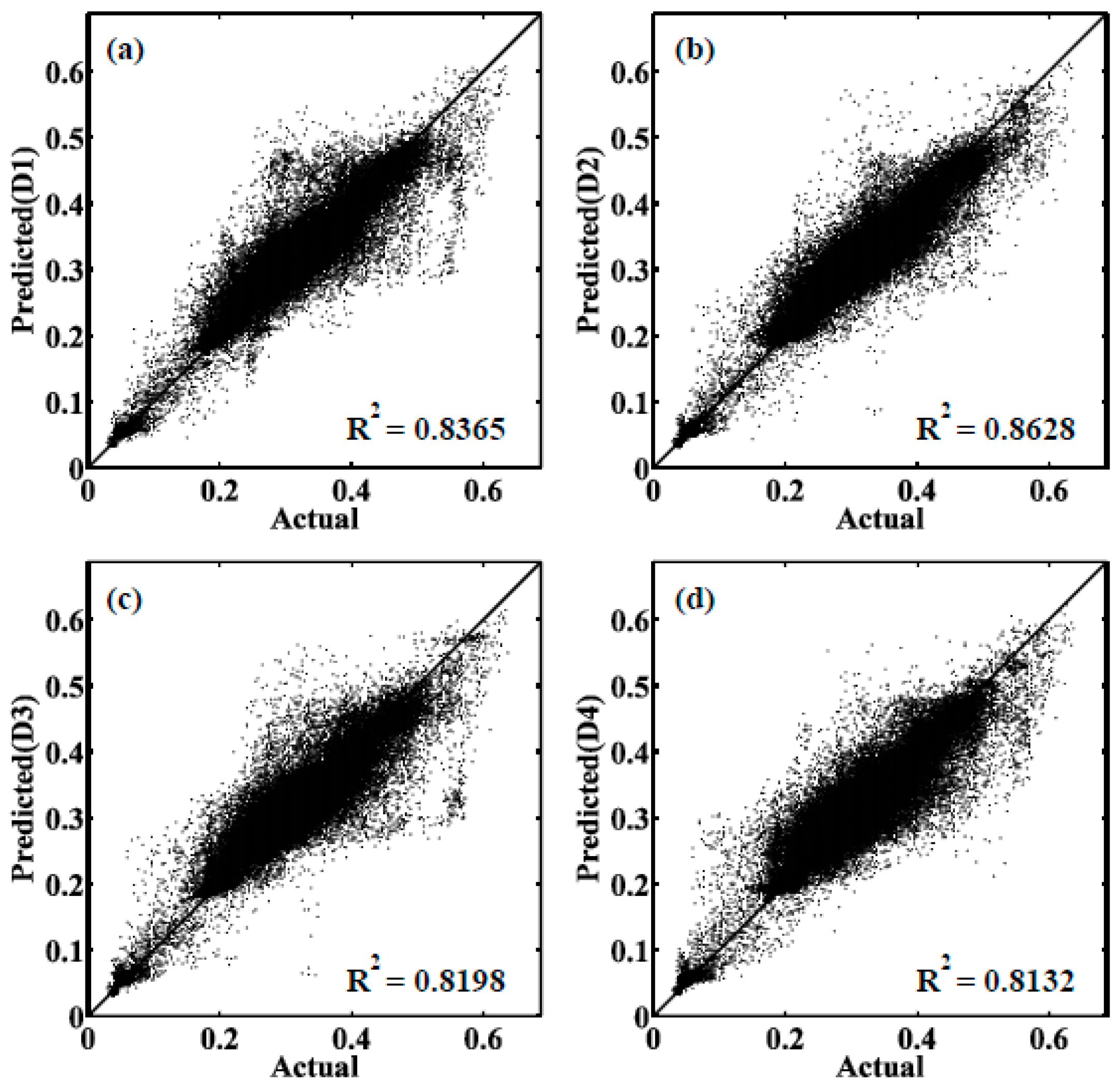
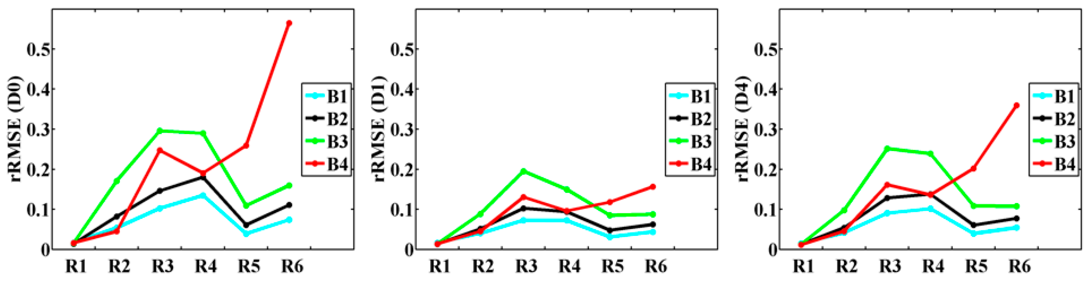
3.2. Comparison of Multi-Temporal Influence of Training Imagery

Given the often non-stationary nature of land surface changes, it might be expected that temporally closer input images should provide the foundation for a more accurate simulation response. To confirm this hypothesis, R3 (the region covered by dense farmland) is once again used as a representative example to assess the temporal influence on gap-filling. As discussed in Section 3.1, the gap-filling results of univariate simulations are relatively poorer when compared tothe bivariate cases, and thus only bivariate simulations are used here. The zoomed images of Figure 6 exhibit a decreasing trend of prediction accuracy from B-D1 to B-D4. The edge of the river in B-D1, which uses an input image with a two-week distance, is clearly distinguishable and maintains the same shape as in the actual image despite not being per-pixel accurate. The edge gradually becomes obscured but retains its shape in B-D2 and B-D3, which represent a four-week and six-week distance input image respectively, before becoming completely blurred and less identifiable in B-D4. The input image used in B-D4 is over four months distant from the target date.

The quantitative metrics in Table 4 also indicate a more accurate reproduction using temporally closer input images. For the bivariate cases, since the simulation results are all quite accurate, the statistical changes between the four cases are relatively small, although still exhibiting a decreasing prediction accuracy from B-D1 to B-D4. B-D1, which uses the temporally closest input image, generally gives the lowest RMSE, MSA, rRMSE and MdAPE and the highest R2, with only occasional exceptions, representing a more accurate prediction result. B-D4, which implements the temporally farthest input image for filling gaps, always provides the highest RMSE, MSA, rRMSE and MdAPE and lowest consistency between the predicted and actual values (R2). The scatterplots of band 4 shown in Figure 7 also present a narrower range of scatter in B-D1 and B-D2 than in B-D3 or B-D4. When a comparison of these statistical indices is applied to other land cover types, similar features can also be observed, with B-D1 and D2 performing better than B-D3, while B-D4 provides the poorest results (Tables S1–S5). One exception to be noted is the desert area (Figure S1), in which B-D1 provides less accurate results than B-D4, although the values do not vary much. The anomalous result is somewhat expected, as the land surface feature of D1 (two-week distance) is less similar to the target image when compared to the other input images.

Overall, assessments from both qualitative and quantitative perspectives demonstrate that temporally closer training images have a positive influence on the fidelity of simulation results by providing a more accurate prediction. For homogeneous areas, the temporal impact of input images on gap-filling results is not as significant as for heterogeneous areas. Interestingly, regardless of the temporal distances studied here for the input image, the bivariate simulation invariably provides acceptable results.

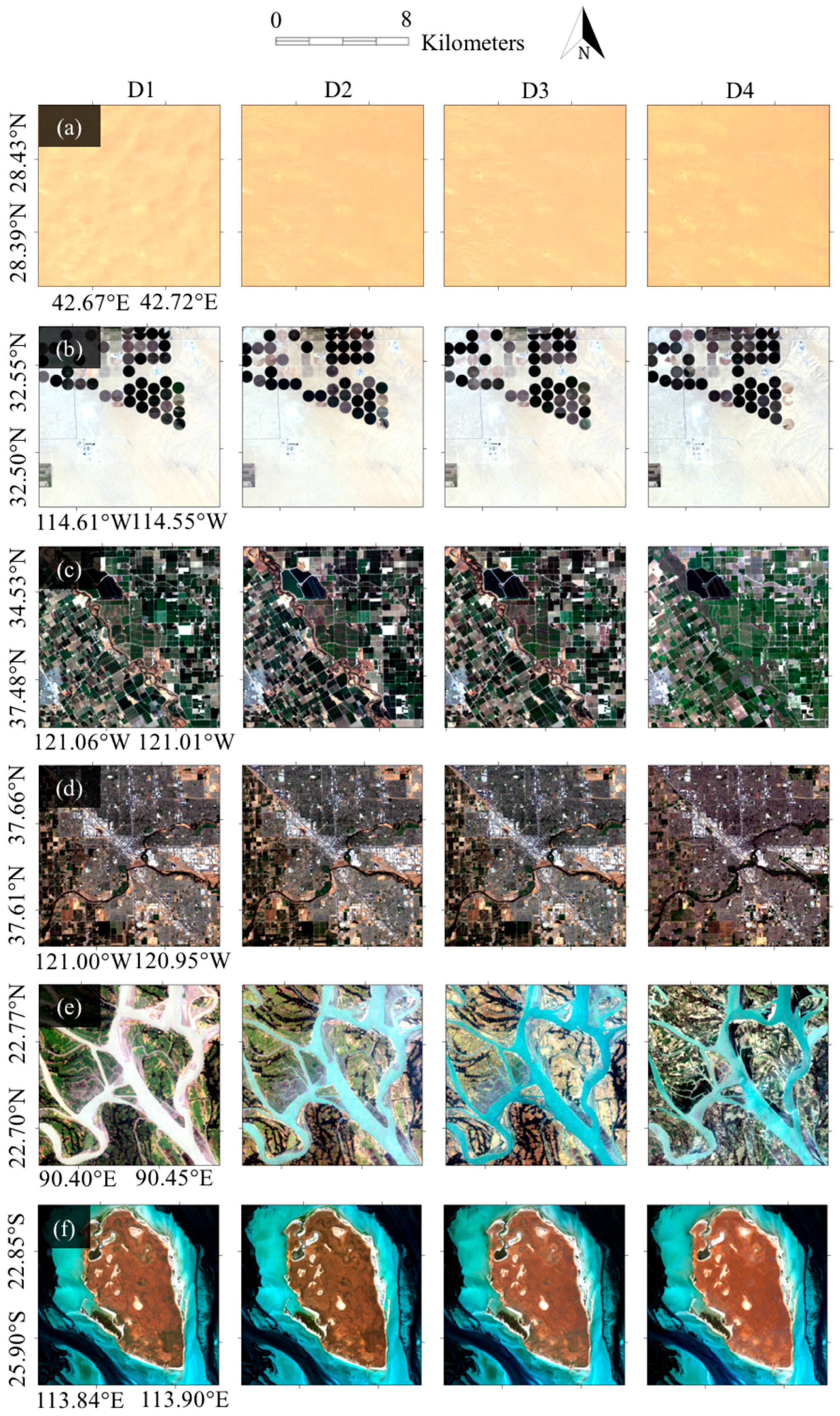
3.3. Impact of Heterogeneity on Reconstructions

The six regions studied in this paper can be ranked from homogeneous (desert, R1), relatively homogeneous (sparse agricultural, R2), heterogeneous (dense farmland, R3 and urban, R4) to special landscapes with dramatic discontinuity features (braided river, R5 and coastal, R6). It was anticipated that the more homogeneous the landscape is, the more accurate the reconstructed result should be, i.e., a gap-filled desert should produce the most accurate result among all regions studied here. Furthermore, for homogeneous areas, U-D0 (which uses non-gap location within the target image to fill gap locations) should provide a sufficiently accurate reproduction, while for heterogeneous areas, the bivariate simulation should provide a more satisfactory result. As introduced in Section 1, one issue that constrains the application of many other gap-filling approaches is the inability to accurately predict discontinuity features and narrow image elements such as streams. Here, the capacity of the Direct Sampling method in predicting such features is examined, with scenarios U-D0 (the best univariate), B-D1 (the best bivariate) and B-D4 (the poorest bivariate) selected to further evaluate the impact of heterogeneity on gap-filling.

Quantitative statistical metrics such as the mean reflectance, standard deviation and skew of band 4 of the target images, together with the filled results for each of the six land cover types, are listed in

Table 5. Summary statistics of band 4 for the target images and filled results of six studied regions.

	Case Name	Mean	St. Dev.	Skew
Desert	Actual	0.4891	0.0125	−0.0980
	U-D0	0.4891	0.0116	−0.2304
	B-D1	0.4890	0.0117	−0.1899
	B-D4	0.4890	0.0119	−0.1363
Sparse agricultural	Actual	0.3782	0.0413	2.1496
	U-D0	0.3782	0.0400	2.2386
	B-D1	0.3783	0.0402	2.2373
	B-D4	0.3783	0.0404	2.2537
Dense farmland	Actual	0.3132	0.0910	−0.1222
	U-D0	0.3134	0.0879	−0.1246
	B-D1	0.3138	0.0891	−0.2066
	B-D4	0.3134	0.0886	−0.1754
Urban area	Actual	0.2714	0.0576	0.8012
	U-D0	0.2717	0.0530	0.8884
	B-D1	0.2714	0.0553	0.8240
	B-D4	0.2710	0.0538	0.8818
Braided river	Actual	0.1854	0.0901	−0.3713
	U-D0	0.1858	0.0887	−0.4269
	B-D1	0.1848	0.0888	−0.4063
	B-D4	0.1853	0.0889	−0.4196
Coastal area	Actual	0.1147	0.1267	0.6625
	U-D0	0.1150	0.1247	0.6331
	B-D1	0.1145	0.1263	0.6482
	B-D4	0.1153	0.1266	0.6347

to evaluate the overall prediction accuracy. From Table 5, it is clear that for all examined regions, the Direct Sampling can fill the gaps reasonably, providing comparable statistical metrics as those calculated using the non-gapped image. Among the simulation cases, B-D1 generally provides closer values than other simulation cases. To compare the prediction accuracy over different landscapes, the rRMSE values of bands 1–4 for the six studied regions are displayed in Figure 8. The rRMSE of bands 5 and 7 for R3 (dense farmland), R5 (braided river) and R6 (coastal) are much larger (refer to Table 4, Tables S4 and S5) than bands 1–4 and are not included in the figures. The large rRMSE values do not systematically represent a poor gap-filling result, with a possible explanation for this response being that the prediction errors are large at locations whose actual reflectance values are small. In Figure 8, for all three selected cases, the rRMSE shows an increasing trend as the landscape heterogeneity becomes more complex from R1 (desert) to R2 (sparse agricultural) and then to R3 (dense farmland), across all of the examined bands. The rRMSE values of R3 (dense farmland) and R4 (urban) are almost at the same level. rRMSE values in R5 (braided river) and R6 (coastal) are close for bands 1–3, but when it comes to band 4, the rRMSE values of both regions become very large, with R6 larger than any of the other regions. MdAPE of all the tested regions and bands are shown in Table 4. The conclusion deduced from MdAPE is similar to rRMSE, with an increasing tendency from R1 to R2 to R3 as the landscape complexity increases. The performance of the Direct Sampling over R3 and R4 is similar. Gap-filling over R5 and R6 provides similar prediction accuracy for bands 1–4, while the MdAPE values for bands 5 and 7 become very large. One issue to be mentioned is that the prediction accuracy provided by bivariate simulations (B-D1 and B-D4) are improved dramatically when compared with the univariate simulation (U-D0) for relatively heterogeneous regions such as R4 (urban). For instance, the rRMSE values of case B-D1 of R4 is almost half that for case U-D0 for all bands. However, for R1 (desert), a strongly homogeneous area, the improvement from univariate to bivariate simulation can be observed, but not significant.

Overall, it is reasonable to conclude that for homogeneous areas, satisfactory simulation results can be obtained without the need for additional input images (i.e., the U-D0 case). This is not so for more heterogeneous areas, where such an implementation present results that are merely acceptable. For increasingly complex landscapes, employing the univariate case may fail to produce realistic results and the multivariate methodology then needs to be considered.

4. Discussion

The results of our analysis illustrate that the Direct Sampling method performs satisfactorily in filling Landsat 7 gaps for most land cover areas, with an accuracy varying across the different land cover types. Homogeneous to relatively homogeneous sites such as deserts and sparse rural areas are reproduced most accurately, even when using only the non-gap locations in the target image (i.e., without using any other input or auxiliary image). Indeed, when filling gaps located in homogeneous or relatively homogeneous areas, there is often no need to introduce additional input images to inform the training procedure, since the information provided by known areas within the target image may be sufficient to produce acceptable results. When the Direct Sampling is applied to heterogeneous areas including dense farmland and urban locations, an accurate result can be achieved through the use of bivariate simulation. Bivariate simulation provides much more accurate results compared to univariate simulation, regardless of whether the reflectance values of the input image differ from the target image. Furthermore, image features such as narrow rivers or streams exhibited in braided river and coastal areas can be well reproduced through bivariate simulation, although they can potentially suffer from per-pixel accuracy (i.e., global features are retained, but local features may be diminished). Although not discussed directly in this analysis, it was found that a tri-variate simulation produced even more accurate results, relative to the univariate and bivariate cases, reinforcing the value of additional information content in the gap-filling process.

As expected, the impact of temporally adjacent data in the auxiliary image diminishes with distance from the target image collection. Interestingly, in cases where there is a lack of temporally close input imagery, even an input image from a totally different season was able to produce an acceptable result. The flexibility in the input image requirements is one of the key advantages of the Direct Sampling. Due to the approximately 16 day sun-synchronous orbital return interval of Landsat satellites, it is quite possible that a temporally close and cloud-free input image may be unavailable. As such, applying imagery from other remote sensors is an appealing alternative in comparison to relying on imagery from any individual satellite system alone. Both Landsat 5 and Landsat 8 are possible solutions to sourcing additional imagery for gap-filling purposes in Landsat 7 imagery. While Landsat 8 has only been in orbit since February 2013, Landsat 5 provided data for the period since scan line failure until it was decommissioned in November 2011. For this satellite, the data acquired by the Thematic Mapper (TM) sensor is similar to the Landsat 7 Enhanced Thematic Mapper Plus (ETM+) and the Landsat 8 Operational Land Imager (OLI), with overlapping wavelengths and resolution across many of the spectral bands. The radiometric cross-calibration of the Landsat 7 ETM+ and Landsat 5 TM sensors can be operated based on the methodology of Teillet at al. [33] and corresponding calibration of Landsat 8 OLI and Landsat 7 ETM+ based on Mishra et al. [34]. The imagery acquired by both Landsat 5 and Landsat 8 usually has an eight-day interval with Landsat 7 imagery, which is shorter than the sixteen-day continuous observation interval of Landsat 7. Apart from available Landsat platforms, many other sensors can be employed to provide information for gap-filling, despite spectral band and spatial resolution differences. A number of studies have explored the option of using other sensors to fill gaps, such as Moderate-Resolution Imaging Spectroradiometer (MODIS) [35], Advanced Spaceborne Thermal Emission and Reflection Radiometer (Aster) [36], Indian Remote Sensing Satellite (IRS) [37], China Brazil Earth Resources Satellite (CEBRS) [38] and have demonstrated the possibility of using such sensors to compensate for the gap region. Exploiting the potential of Landsat and other multi-sensor platforms is the focus of continuing research.

Although not comprehensively examined here, an advantage of the Direct Sampling method is the rapid computational speed. The rRMSE of most of the bivariate cases tested here have similar values to those presented in Pringle et al. [8]. A key difference however is the computing time. In the present study, simulations were run using a Windows system on an Intel Core i7 2.80 GHz processor with 16 GB of RAM. Each target image has 48,617 pixels requiring gap-filling. For univariate simulations except U-D0, each reconstruction takes just a few seconds, while for U-D0 it takes approximately six minutes for each reconstruction. Bivariate simulations required 25 min for each reconstruction (about four hours for all 10reconstructions). In the study of Pringle et al. [8], a Linux operating system with a Xeon 2.33 GHz processor and 48 GB of RAM required a computation time of approximately 12 h for 5000 missing pixels.

5. Conclusions

The failure of the SLC on Landsat 7 imposed some obvious constraints on the application of the satellite data across local-to-global scales, especially in efforts to develop an uninterrupted and spatially continuous time-series of land surface change. Despite a range of methods that have been proposed for gap-filling purposes since the instrument failure, all have their constraints, including limited application to heterogeneous regions or computational cost. Identifying an approach that can be used across a wide range of landscapes, that is easy to implement and can be made accessible to users, is an area of needed research. Here we explore the development of the Direct Sampling method for gap-filling purposes. Results indicate that the method provides satisfactory simulations over a range of landscapes of varying land surface heterogeneity. For homogeneous landscapes, it was found that the univariate simulation that used non-gap locations in the target image (i.e., without requiring additional input imagery) provided an accurate gap-filling result. For more heterogeneous areas, bivariate simulations using an input image acquired at another date provided satisfactory results, in spite of input image separation varying temporally from a few weeks to four months from the target acquisition. However, a temporally closer input image generally improved the prediction accuracy relative to one that was further displaced in time.

While the capacity of the Direct Sampling for filling SLC off imagery has been demonstrated, a comparison with other gap-filling approaches is required. A comprehensive inter-comparison exercise assessing the MPS approach against other common gap-filling approaches is currently underway. Preliminary results indicate that one of the key advantages of the Direct Sampling approach is that it can be used for filling gaps when there is no covariate information available (i.e., the U-D0 case discussed in this study). Such an advantage proves useful in filling gaps when abrupt changes have occurred within a landscape: for instance, in response to rapid land clearing, tsunamis or bushfires. An issue that also requires further consideration relates to the uniform prescription of selected parameter values for all land cover types. This was imposed in order to allow a comparison of the performance of the Direct Sampling across these different land covers. However, in a real-world application of the approach, a more specific selection of parameters according to the training and target imagery used in the simulation process is recommended, which will no doubt produce improved results. The possibility of achieving per-pixel accuracy for heterogeneous landscapes depends highly on the selection of parameters and not only on the input image used. Ongoing investigations are currently exploring a user-friendly method to provide optimized parameters based on the specific training and target image used, in addition to employing ancillary data-sets for gap-filling.

References

1. Landsat; National Aeronautics and Space Administration (NASA). Landsat 7 Science Data Users Handbook. Available online: http://landsat.gsfc.nasa.gov/wp-content/uploads/2016/08/Landsat7_Handbook.pdf (accessed on 11 March 2011).
2. United States Geological Survey (USGS). Landsat-A Global Land-Imaging Mission: Geological Survey Fact Sheet 2012-3072. Available online: https://pubs.usgs.gov/fs/2012/3072/ (accessed on 19 July 2012).
3. United States Geological Survey (USGS). Preliminary Assessment of Landsat 7 ETM+ Data Following Scan Line Corrector Malfunction. Available online: https://landsat.usgs.gov/sites/default/files/documents/SLC_off_Scientific_Usability.pdf (accessed on 16 July 2003).
4. Scaramuzza, P.; Micijevic, E.; Chander, G. SLC Gap-Filled Products Phase One Methodology. 2004. Available online: https://landsat.usgs.gov/sites/default/files/documents/SLC_Gap_Fill_Methodology.pdf (accessed on 18 March 2004). [Google Scholar]
5. Scaramuzza, P.; Micijevic, E.; Chander, G. Phase 2 Gap-Fill Algorithm: SLC-off Gap-Filled Products Gap-Filled Algorithm Methodology. 2004. Available online: https://landsat.usgs.gov/sites/default/files/documents/L7SLCGapFilledMethod.pdf (accessed on 7 October 2004). [Google Scholar]
6. Maxwell, S.K.; Schmidt, G.L.; Storey, J.C. A multi-scale segmentation approach to filling gaps in Landsat ETM+ SLC-off images. Int. J. Remote Sens. 2007, 28, 5339–5356. [Google Scholar] [CrossRef]
7. Flanders, D.; Hall-Beyer, M.; Pereverzoff, J. Preliminary evaluation of eCognition object-based software for cut block delineation and feature extraction. Can. J. Remote Sens. 2003, 29, 441–452. [Google Scholar] [CrossRef]
8. Pringle, M.J.; Schmidt, M.; Muir, J.S. Geostatistical interpolation of SLC-off Landsat ETM+ images. ISPRS J. Photogramm. Remote Sens. 2009, 64, 654–664. [Google Scholar] [CrossRef]
9. Chiles, J.P.; Delfiner, P. Geostatistics: Modeling Spatial Uncertainty; John Wiley & Sons: Hoboken, NJ, USA, 2009. [Google Scholar]
10. Goovaerts, P. Geostatistics for Natural Resources Evaluation; Oxford University Press: Oxford, UK, 1997. [Google Scholar]
11. Chen, J.; Zhu, X.; Vogelmann, J.E.; Gao, F.; Jin, S. A simple and effective method for filling gaps in Landsat ETM+ SLC-off images. Remote Sens. Environ. 2011, 115, 1053–1064. [Google Scholar] [CrossRef]
12. Zhu, X.; Liu, D.; Chen, J. A new geostatistical approach for filling gaps in Landsat ETM+ SLC-off images. Remote Sens. Environ. 2012, 124, 49–60. [Google Scholar] [CrossRef]
13. Zeng, C.; Shen, H.; Zhang, L. Recovering missing pixels for Landsat ETM+ SLC-off imagery using multi-temporal regression analysis and a regularization method. Remote Sens. Environ. 2013, 131, 182–194. [Google Scholar] [CrossRef]
14. Guardiano, F.B.; Srivastava, R.M. Multivariate geostatistics: beyond bivariate moments. In Geostatistics Troia’92; Springer: Dordreche, The Netherlands, 1993; Volume 1, pp. 133–144. [Google Scholar]
15. Mariethoz, G.; Caers, J. Multiple-Point Geostatistics: Stochastic Modeling with Training Images; Wiley Blackwell: Hoboken, NJ, USA, 2014. [Google Scholar]
16. Strebelle, S. Conditional simulation of complex geological structures using multiple-point statistics. Math. Geol. 2002, 34, 1–21. [Google Scholar] [CrossRef]
17. Arpat, G.B.; Caers, J. A multiple-scale, pattern-based approach to sequential simulation. In Geostatistics Banff 2004; Springer: Dordreche, The Netherlands, 2005; pp. 255–264. [Google Scholar]
18. Daly, C. Higher order models using entropy, Markov random fields and sequential simulation. In Geostatistics Banff 2004; Springer: Dordreche, The Netherlands, 2005; pp. 215–224. [Google Scholar]
19. Zhang, T.; Switzer, P.; Journel, A. Filter-based classification of training image patterns for spatial simulation. Math. Geol. 2006, 38, 63–80. [Google Scholar] [CrossRef]
20. Hurley, N.F.; Zhang, T. Method to generate full-bore images using borehole images and multipoint statistics. SPE Reserv. Eval. Eng. 2011, 14, 204–214. [Google Scholar] [CrossRef]
21. Okabe, H.; Blunt, M.J. Multiple-point statistics to generate pore space images. In Geostatistics Banff 2004; Springer: Dordreche, The Netherlands, 2005; pp. 763–768. [Google Scholar]
22. Wu, J.; Boucher, A.; Zhang, T. A SGeMS code for pattern simulation of continuous and categorical variables: FILTERSIM. Comput. Geosci. 2008, 34, 1863–1876. [Google Scholar] [CrossRef]
23. Tang, Y.; Atkinson, P.M.; Wardrop, N.A.; Zhang, J. Multiple-point geostatistical simulation for post-processing a remotely sensed land cover classification. Spat. Stat. 2013, 5, 69–84. [Google Scholar] [CrossRef]
24. Yong, G.; Hexiang, B.; Qiuming, C. Solution of multiple-point statistics to extracting information from remotely sensed imagery. J. China Univ. Geosci. 2008, 19, 421–428. [Google Scholar] [CrossRef]
25. Boucher, A. Sub-pixel mapping of coarse satellite remote sensing images with stochastic simulations from training images. Math. Geosci. 2009, 41, 265–290. [Google Scholar] [CrossRef]
26. Tang, Y.; Atkinson, P.M.; Zhang, J. Downscaling remotely sensed imagery using area-to-point cokriging and multiple-point geostatistical simulation. ISPRS J. Photogramm. Remote Sens. 2015, 101, 174–185. [Google Scholar] [CrossRef]
27. Mariethoz, G.; McCabe, M.F.; Renard, P. Spatiotemporal reconstruction of gaps in multivariate fields using the direct sampling approach. Water Resour. Res. 2012, 48. [Google Scholar] [CrossRef]
28. Mariethoz, G.; Renard, P.; Straubhaar, J. The direct sampling method to perform multiple-point geostatistical simulations. Water Resour. Res. 2010, 46, 1–14. [Google Scholar] [CrossRef]
29. Jha, S.K.; Mariethoz, G.; Evans, J.; McCabe, M.F.; Sharma, A. A space and time scale-dependent nonlinear geostatistical approach for downscaling daily precipitation and temperature. Water Resour. Res. 2015, 51, 6244–6261. [Google Scholar] [CrossRef]
30. Oriani, F.; Straubhaar, J.; Renard, P.; Mariethoz, G. Simulation of rainfall time series from different climatic regions using the direct sampling technique. Hydrol. Earth Syst. Sci. 2014, 18, 3015–3031. [Google Scholar] [CrossRef]
31. Mariethoz, G.; Renard, P. Reconstruction of incomplete data sets or images using direct sampling. Math. Geosci. 2010, 42, 245–268. [Google Scholar] [CrossRef]
32. Meerschman, E.; Pirot, G.; Mariethoz, G.; Straubhaar, J.; van Meirvenne, M.; Renard, P. A practical guide to performing multiple-point statistical simulations with the Direct Sampling algorithm. Comput. Geosci. 2013, 52, 307–324. [Google Scholar] [CrossRef]
33. Teillet, P.M.; Barker, J.L.; Markham, B.L.; Irish, R.R.; Fedosejevs, G.; Storey, J.C. Radiometric cross-calibration of the Landsat-7 ETM+ and Landsat-5 TM sensors based on tandem data sets. Remote Sens. Environ. 2001, 78, 39–54. [Google Scholar] [CrossRef]
34. Mishra, N.; Haque, M.O.; Leigh, L.; Aaron, D.; Helder, D.; Markham, B. Radiometric cross calibration of Landsat 8 Operational Land Imager (OLI) and Landsat 7 enhanced thematic mapper plus (ETM+). Remote Sens. 2014, 6, 12619–12638. [Google Scholar] [CrossRef]
35. Roy, D.P.; Ju, J.; Lewis, P.; Schaaf, C.; Gao, F.; Hansen, M.; Lindquist, E. Multi-temporal MODIS-Landsat data fusion for relative radiometric normalization, gap filling, and prediction of Landsat data. Remote Sens. Environ. 2008, 112, 3112–3130. [Google Scholar] [CrossRef]
36. Mahmood, T.; Easson, G. Comparing aster and Landsat 7 ETM+ for change detection. In Proceedings of the Annual Conference of the American Society for Photogrammetry and Remote Sensing 2006: Prospecting for Geospatial Information Integration, Reno, NV, USA, 1–5 May 2006; pp. 828–839.
37. Reza, M.M.; Ali, S.N. Using IRS products to recover 7ETM+ defective images. Am. J. Appl. Sci. 2008, 5, 618–625. [Google Scholar] [CrossRef]
38. Chen, F.; Tang, L.; Qiu, Q. Exploitation of CBERS-02B as auxiliary data in recovering the Landsat7 ETM+ SLC-off image. In Proceedings of the 2010 18th International Conference on Geoinformatics, Beijing, China, 18–20 June 2010.
Figure 1. The Direct Sampling approach and its use of a training image to predict a missing pixel in the target image. The procedure follows a number of steps, including (a) definition of the simulation grid, where the pixel x represents the pixel to be filled, and the blue, red, yellow pixels represent pixels with known values; (b) definition of the data event; (c) use of a training image to provide information to fill the gaps, with a search employing the defined data event from (b) until; (d) the simulation data event is identified in the training image; and (e) the missing target value corresponding to the identified training value is assigned the first data point matching the data event.
Remotesensing 09 00012 g001
Figure 2. Flowchart of the Direct Sampling method using a single training image. In the flowchart, x and y are the locations of the pixels in target image and training image respectively. Z(x) and Z(y) are the values at corresponding locations; d is the distance between two data events Nx and Ny, which can be denoted as d{Nx, Ny}. f is the maximum search proportion of scanned training image and t is the user-defined threshold.
Remotesensing 09 00012 g002
Figure 3. Selection of neighborhood pixels for bivariate simulations, with (a) target images and (b) training images of the same two variables. Colored pixels are informed, and gray pixels are unknown. The pixel x is the target pixel to be predicted at the current step. Neighborhood pixels of each variable are selected, composing the data event Nx. Replicate Ny of the data event Nx is marked in red in (b) and will be used to compute the distance.
Remotesensing 09 00012 g003
Figure 4. Target images for each of the studied regions, both with and without imposed gaps, for (a) desert; (b) sparse agricultural; (c) dense farmland; (d) urban; (e) braided river and (f) coastal area.
Remotesensing 09 00012 g004
Figure 5. ETM+ images for the six studied regions and the different temporal images used in analysis (see Table 1), corresponding to (a) desert; (b) sparse agricultural; (c) dense farmland; (d) urban; (e) braided river and (f) coastal area.
Remotesensing 09 00012 g005
Figure 6. Mean realizations and the zoomed images for the nine test cases conducted over R3 (dense farmland). “Actual” is the actual image. “U-” and “B-” represents univariate and bivariate simulation. “D1”–“D4” represent the input images used for filling gaps, and “U-D0” is the univariate simulation without using an additional training image. The areas marked with red square in the mean realizations are magnified to the right of each pair. The location of the gap trace is denoted with an arrow in the mean realization of U-D1, and a red rectangular is marked in all zoomed images at the same location for the edge shape comparison in Section 3.2.
Remotesensing 09 00012 g006
Figure 7. Scatter plots of reflectance values of band 4 for bivariate cases, with (ad) corresponding to B-D1, B-D2, B-D3 and B-D4. X axis reflects the actual reflectance while the Y axis is the predicted reflectance. R2 is the coefficient of determination.
Remotesensing 09 00012 g007
Figure 8. rRMSE values of bands 1–4 of cases U-D0, B-D1 and B-D4 across six tested regions, with B1-B4 corresponding bands, R1 desert, R2 sparse agricultural, R3 dense farmland, R4 urban area, R5 braided river and R6 coastal area.
Remotesensing 09 00012 g008