Improving Land Surface Temperature Retrievals over Mountainous Regions

Abstract

Algorithms for Land Surface Temperature (LST) retrieval from infrared measurements are usually sensitive to the amount of water vapor present in the atmosphere. The Satellite Application Facilities on Climate Monitoring and Land Surface Analysis (CM SAF and LSA SAF) are currently compiling a 25 year LST Climate data record (CDR), which uses water vapor information from ERA-Int reanalysis. However, its relatively coarse spatial resolution may lead to systematic errors in the humidity profiles with implications in LST, particularly over mountainous areas. The present study compares LST estimated with three different retrieval algorithms: a radiative transfer-based physical mono-window (PMW), a statistical mono-window (SMW), and a generalized split-windows (GSW). The algorithms were tested over the Alpine region using ERA-Int reanalysis data and relied on the finer spatial scale Consortium for Small-Scale Modelling (COSMO) model data as a reference. Two methods were developed to correct ERA-Int water vapor misestimation: (1) an exponential parametrization of total precipitable water (TPW) appropriate for SMW/GSW; and (2) a level reduction method to be used in PMW. When ERA-Int TPW was used, the algorithm missed the right TPW class in 87% of the cases. When the exponential parametrization was used, the missing class rate decreased to 9%, and when the level reduction method was applied, the LST corrections went up to 1.7 K over the study region. Overall, the correction for pixel orography in TPW leads to corrections in LST estimations, which are relevant to ensure that long-term LST records meet climate requirements, particularly over mountainous regions.

1. Introduction

Land surface temperature (LST) is a crucial variable for environmental and climate studies. Together with surface emissivity, LST controls the surface’s upward thermal radiation. LST also partly controls the surface’s turbulent heat flux, which modulates the thermodynamic structure of the atmospheric boundary layer [1]. Several studies pointed out the importance of LST in a range of applications, such as general model assessment [2,3], data assimilation [4,5,6,7,8], hydrology [9,10], and climate monitoring [11,12], among others.

Taking into account the growing interest in LST as an essential climate variable, the Satellite Application Facilities on Climate Monitoring and Land Surface Analysis (CM SAF and LSA SAF) are currently compiling a 25 year LST Climate data record (CDR) with hourly temporal and 0.05 degree spatial resolutions [11], using brightness temperatures measured by the European Organisation for the Exploitation of Meteorological Satellites (EUMETSAT) Meteosat First Generation (MFG) and Meteostat Second Generation (MSG) satellites. The atmospheric correction makes use of profiles of water vapor and temperature extracted from the European Centre for Medium-Range Weather Forecasts (ECMWF) reanalyses, namely ERA-Interim (hereafter ERA-Int), a global atmospheric reanalysis from 1979, continuously updated in real time [13]. One of the main advantages of such an LST dataset is its high homogeneity, since the retrieval algorithm and ancillary data used are the same for the whole processing period, and the process makes use of recent EUMETSAT efforts to recalibrate top-of-atmosphere radiances.

A main interest in such long records of remotely sensed LST is to complement the widely used near-surface air temperature in situ measurements in climate monitoring applications [14,15]. In-situ data present large gaps and uncertainties where station density is low, e.g., over sparsely populated areas like deserts and mountains. According to a recent study [16], there is growing evidence that the rate of warming is amplified with elevation. However, it has been extremely difficult to define the rate of warming in mountainous regions due to the lack of surface in situ measurements at high elevation sites [17]. This issue may be overcome by using long-term time series of spatially continuous remotely sensed LST datasets. A study addressing the rapid warming over the Tibetan plateau using nighttime Moderate Resolution Imaging Spectro-radiometer (MODIS) data and station observations [18] may be viewed as a first step in this direction; however, the added value of LST crucially depends on the quality of the dataset over such areas.

LST is usually retrieved from remote sensors using data from one or more channels within the thermal infrared window of the electromagnetic spectrum [19,20,21]. LST retrieval algorithms are usually sensitive to the amount of water vapor in the atmosphere [20,22], which is an input either in the form of water vapor profiles in the case of physical retrievals or of total precipitable water (TPW), which is generally used by statistical methods. This information is often obtained from numerical weather prediction (NWP) models or reanalysis. Because they provide the most stable and consistent information over long periods of time, reanalyses are preferred in the development of CDRs but their relatively coarse spatial resolution (currently of the order of 80 km) may lead to systematic errors in the humidity profiles, particularly over mountainous areas with implications in LST CDRs over such regions.

In this study, we address the problem of water vapor misestimation when using ERA-Int data at high altitudes and its implications in the retrieval of LST. We also develop orographic correction models with the aim of reducing the propagation of error in LST estimates due to water vapor misestimation.

The structure of this paper is organized as follows: in Section 2 the satellite and model data are described, as well as the LST retrieval algorithms used for the study; here, the problem of ERA-Int water vapor misestimation is addressed and the methods to overcome this problem are introduced; in Section 3 the methods developed in Section 2 are applied, and LST estimates with and without them are compared for the chosen retrieval algorithms; finally, Section 4 summarizes the main conclusions of this work.

2. Data and Methods

2.1. Data

2.1.1. Study Area

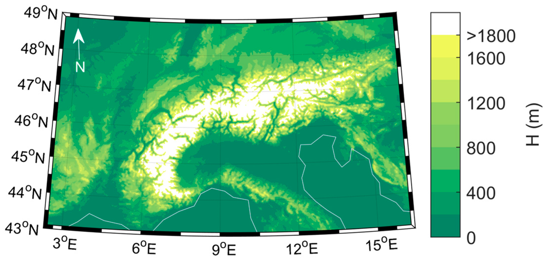
The study focused on the Alpine region, which is the highest and most extensive mountain range in Europe. The Alps are within the MSG/Spinning Enhanced Visible and Infrared Imager (SEVIRI) disk and are part of the domain of the high resolution Consortium for Small-Scale Modelling (COSMO) numerical weather prediction model run at the Swiss Federal Office of Meteorology and Climatology, MeteoSwiss (Figure 1). The Alps were, therefore, our testbed to assess the impact errors in LST retrievals associated with misrepresentation of atmospheric profiles and/or total water vapor content associated with altitude. We used profiles both from high (about 2 km COSMO) and medium (about 80 km ERA-Int) spatial resolution NWP runs. The data corresponded to 6-hourly fields for 1 day per month over the full year of 2014, covering the area shown in Figure 1; however, due to the particularly high cloud frequency over the Alpine region, no data were analyzed for October.

2.1.2. Satellite Data

We considered LST estimates from Top-of-Atmosphere (TOA) brightness temperatures measured by the Spinning Enhanced Visible and Infrared Imager (SEVIRI) onboard the EUMETSAT MSG satellite. SEVIRI is the primary MSG instrument and has the capability to observe the Earth in 12 spectral channels, with view zenith angles (VZA) ranging from 0° to 80°, and with a temporal resolution of 15 min and a spatial resolution of 3-km at the subsatellite point. MSG-3 top-of-atmosphere 10.8 μm and 12.0 μm brightness temperatures, as well as the respective cloud mask, are provided by the LSA SAF. Cloud masks were determined using the software developed by the SAF in support of Nowcasting and Very Short-Range Forecasting (NWC SAF) following the algorithm described by [23]. The LSA SAF also provided surface emissivity values for the split-window channels (centered at 10.8 μm and 12.0 μm) which are obtained via a combination of land cover classification and SEVIRI-based fraction of vegetation cover updated daily on a pixel-by-pixel basis [22,24].

2.1.3. Model Data

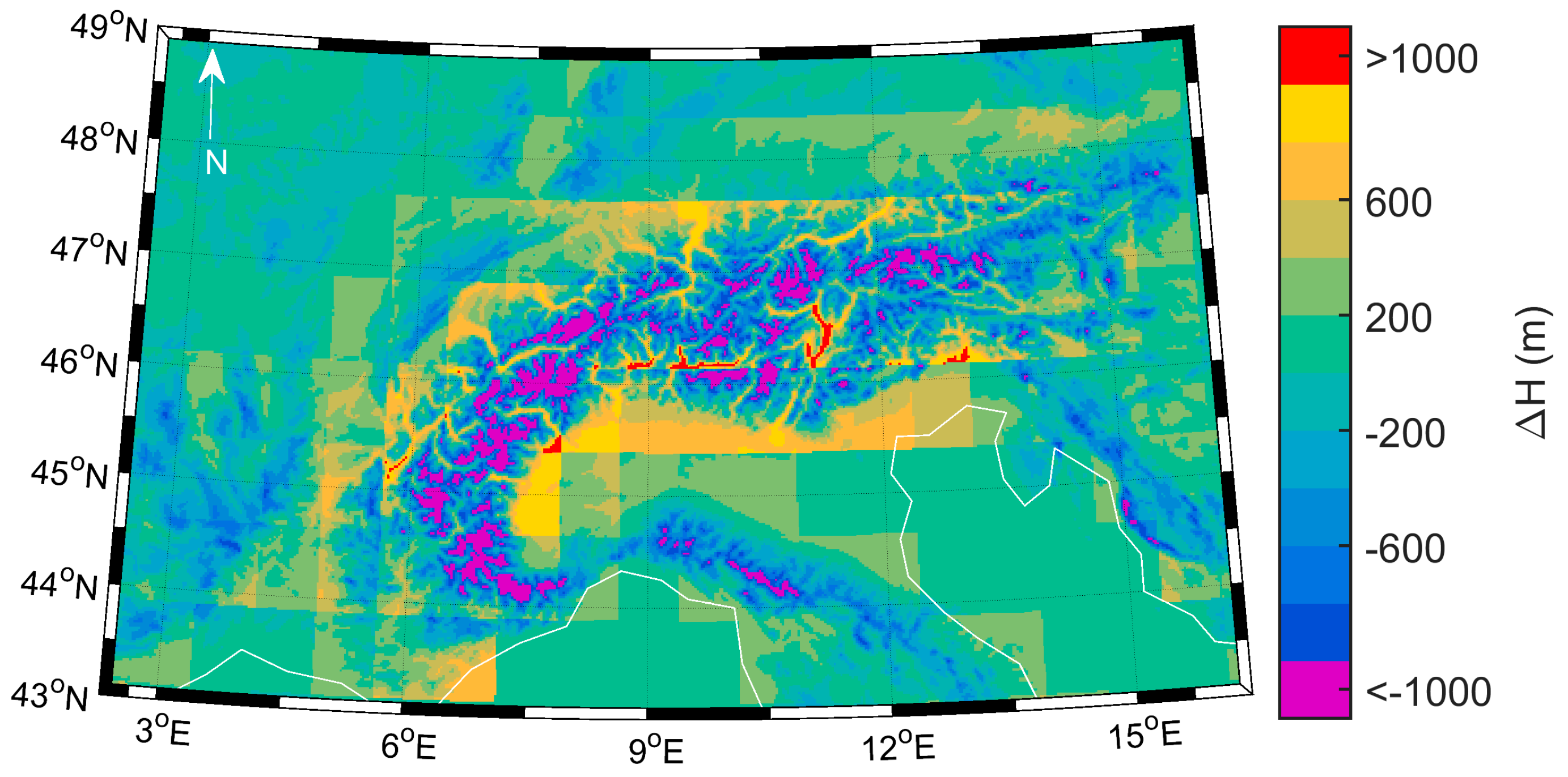
The LST algorithm that is currently being developed by the CM SAF makes use of ERA-Int water vapor and temperature profiles at 60 pressure levels with a horizontal resolution of 80 km [13]. The base altitude for these profiles is defined by a relatively coarse orographic field representative of the model spatial resolution. For mountainous regions, departures of ERA-Int height from actual topography can be very large, and in the Alps these differences can reach 2500 m in a reduced number of locations (Figure 2).

The COSMO model is a non-hydrostatic operational weather prediction model maintained and continuously improved by the national weather services affiliated with the consortium for small-scale modelling (COSMO) [25]. The COSMO model run at MeteoSwiss has a high-resolution topography (of about 2 km), which makes it more suitable to be used as the reference orography field. Furthermore, the small horizontal scale fluctuations of humidity profiles are expected to be more realistically represented in such a high-resolution model.

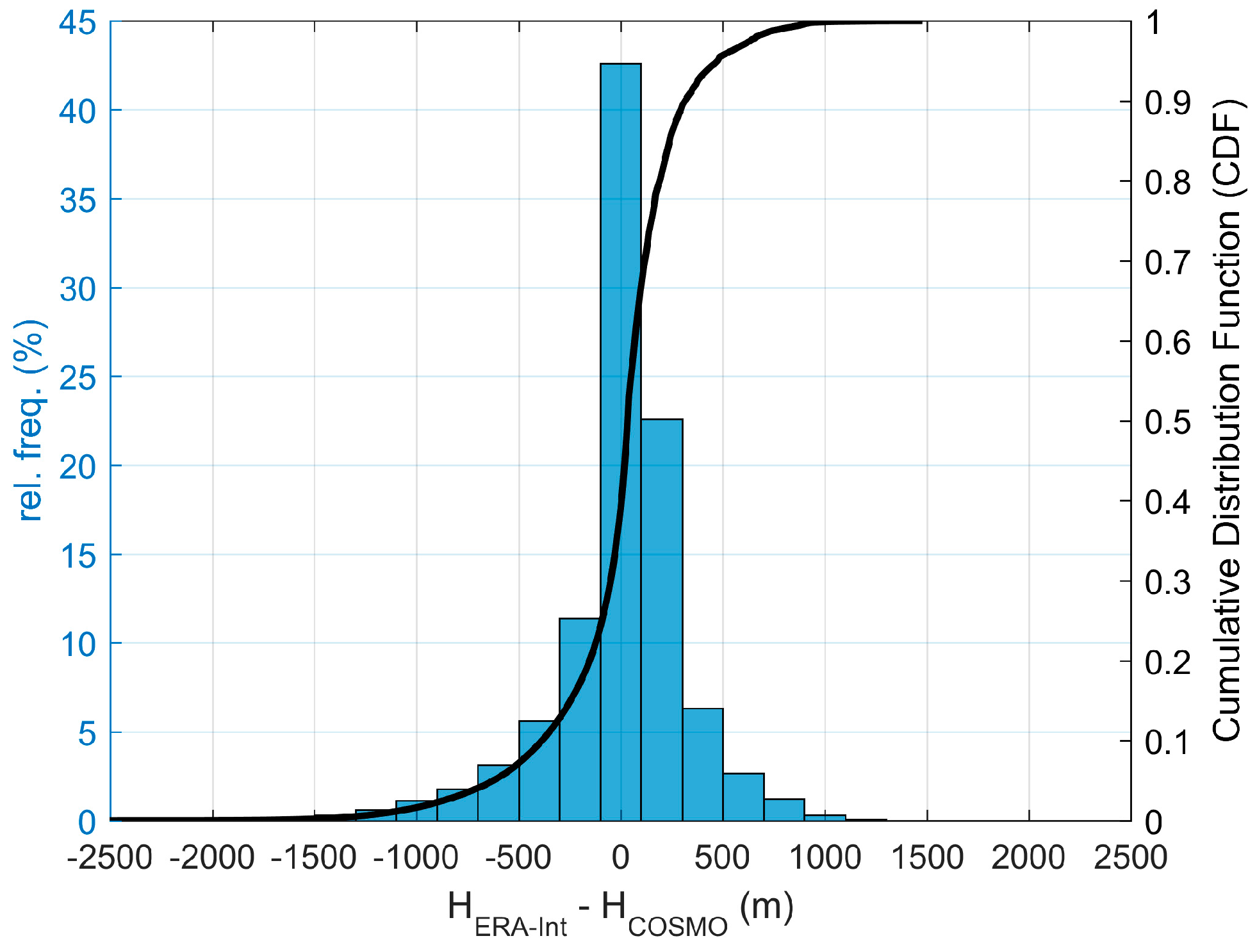
The differences between COSMO and ERA-Int surface orography fields are shown in Figure 2, which clearly puts into evidence the finer details represented in the former. Figure 3 shows that, if COSMOS’s grid cells are taken to be a realistic representation of surface orography, then out of the totality of pixels, the number of cases where ERA-Int underestimates surface height by more than 1000 m is of 2974 pixel locations over the area of study, leading to a sample of 43,096 retrieved LST values covering the year 2014. Overestimation is less frequent, with only 241 pixel locations where ERA-Int surface height is higher than that of COSMO’s by 1000 m or more. This asymmetry results from the smoothing of the topography performed for numerical stability reasons in medium resolution models, and is stronger in those used to build reanalyses datasets. As will be further discussed below, this smoothing may lead to systematic errors in LST estimates over high elevation areas which make use of such reanalyses profiles.

2.2. LST Retrieval Algorithms

A variety of LST retrieval algorithms may be found in the literature (see [19,20,21] for a comprehensive description). Here, we restrict our discussion to the three following approaches:

• Generalized Split-Windows (GSW) is based on the formulation by Wan and Dozier for the Advanced Very High Resolution Radiometer (AVHRR) and MODIS sensors [26] and later adapted for MSG/SEVIRI [22,27,28]; LST is computed using a semi-empirical expression involving top-of-atmosphere brightness temperature and surface emissivity in two thermal infrared channels (10.8 and 12 µm), the so-called split-window channels:

  $$\mathrm{LST}=\left({\mathrm{A}}_1+{\mathrm{A}}_2\frac{1-\mathsf{\epsilon }}{\mathsf{\epsilon }}+{\mathrm{A}}_3\frac{\mathsf{\Delta }\mathsf{\epsilon }}{{\mathsf{\epsilon }}^2}\right)\frac{{\mathrm{T}}_{10.8}+{\mathrm{T}}_{12}}{2}+\left({\mathrm{B}}_1+{\mathrm{B}}_2\frac{1-\mathsf{\epsilon }}{\mathsf{\epsilon }}+{\mathrm{B}}_3\frac{\mathsf{\Delta }\mathsf{\epsilon }}{{\mathsf{\epsilon }}^2}\right)\frac{{\mathrm{T}}_{10.8}-{\mathrm{T}}_{12}}{2}+\mathrm{C},$$

  (1)

  where ${\mathrm{T}}_{10.8}$ and ${\mathrm{T}}_{12}$ are the brightness temperatures in channels 10.8 and 12 µm, respectively, $\epsilon =\frac{{\epsilon }_{10.8}+{\epsilon }_{12}}{2}$ and $\mathsf{\Delta }\mathsf{\epsilon }={\mathsf{\epsilon }}_{10.8}-{\mathsf{\epsilon }}_{12}$ are, respectively, the mean of and the difference between surface emissivities, ${\mathsf{\epsilon }}_{10.8}$ and ${\mathsf{\epsilon }}_{12}$, in the two considered channels, and ${\mathrm{A}}_{\mathrm{i}}$, ${\mathrm{B}}_{\mathrm{i}}$, (i = 1, 2, 3), and C are coefficients calibrated for classes of TPW and VZA [29].
• Statistical Mono-Window (SMW) [11], where LST is computed based on an expression involving TOA brightness temperature and emissivity in a single thermal infrared channel (centered at 10.8 μm):

  $$\mathrm{LST}=\mathrm{A}\frac{{\mathrm{T}}_{\mathrm{c}}}{{\mathsf{\epsilon }}_{\mathrm{c}}}+\mathrm{B}\frac{1}{{\mathsf{\epsilon }}_{\mathrm{c}}}+\mathrm{C},$$

  (2)

  where ${\mathrm{T}}_{\mathrm{c}}$ and ${\mathsf{\epsilon }}_{\mathrm{c}}$ are the brightness temperature and the surface emissivity of the considered channel, respectively, and A, B, and C are coefficients calibrated for different classes of TPW and VZA [29].
• Physical Mono-Window (PMW) [11,30], which is based on the direct inversion of the radiative transfer equation for one channel in the thermal infrared window (again centered at 10.8 μm):

  $$\mathrm{LST}\approx \left(\frac{{\mathrm{c}}_2{\mathsf{\nu }}_{\mathrm{c}}}{\ln \left(\frac{{\mathrm{c}}_1{\mathsf{\nu }}_{\mathrm{c}}^3{\mathsf{\tau }}_{\mathrm{c}}\left(\mathsf{\theta }\right){\mathsf{\epsilon }}_{\mathrm{c}}}{{\mathrm{L}}_{\mathrm{c}}\left(\mathsf{\theta }\right)-{\mathrm{L}}_{\mathrm{c}}^{\mathrm{up}}\left(\mathsf{\theta }\right)-{\mathrm{L}}_{\mathrm{c}}^{\mathrm{dn}}\left(1-{\mathsf{\epsilon }}_{\mathrm{c}}\right){\mathsf{\tau }}_{\mathrm{c}}\left(\mathsf{\theta }\right)}+1\right)}-\mathsf{\beta }\right)/\mathsf{\alpha },$$

  (3)

  where ${\mathsf{\epsilon }}_{\mathrm{c}}$, ${\mathsf{\tau }}_{\mathrm{c}}$, ${\mathrm{L}}_{\mathrm{c}}$, ${\mathrm{L}}_{\mathrm{c}}^{\mathrm{up}}$, ${\mathrm{L}}_{\mathrm{c}}^{\mathrm{dn}}$ are, respectively, the surface emissivity, atmospheric transmissivity, top-of-atmosphere radiance, upward atmospheric path radiance, and downward atmospheric path radiance for the considered channel, ${\mathrm{c}}_1$ and ${\mathrm{c}}_2$ are constants from Planck’s law, and α, β are coefficients that depend on the spectral characteristics of the considered channel, and${\mathsf{\nu }}_{\mathrm{c}}$ is the channel central wavenumber. A radiative transfer model is used to estimate ${\mathsf{\tau }}_{\mathrm{c}}$, ${\mathrm{L}}_{\mathrm{c}}^{\mathrm{up}},$ and ${\mathrm{L}}_{\mathrm{c}}^{\mathrm{dn}}$ using information on air temperature and humidity from atmospheric profiles. In this study, the Radiative Transfer for TIROS Operational Vertical Sounder (RTTOV) model is used for this purpose [31].

These three models were chosen due to the fact that the GSW is the operational model used to retrieve LST in the LSA SAF [24] and both mono-window algorithms are being used to produce the 25 year LST CDR at the CM SAF [11].

2.3. Orographic Correction of Atmospheric Profiles

As described above, the three LST algorithms use as input either the total content of water vapor within the column of atmosphere between the surface and the sensor (Equations (1) and (2)), or the actual atmospheric temperature and humidity profiles (used to solve Equation (3)). Here, we will describe two methodologies to account for the correction of the profile surface height:

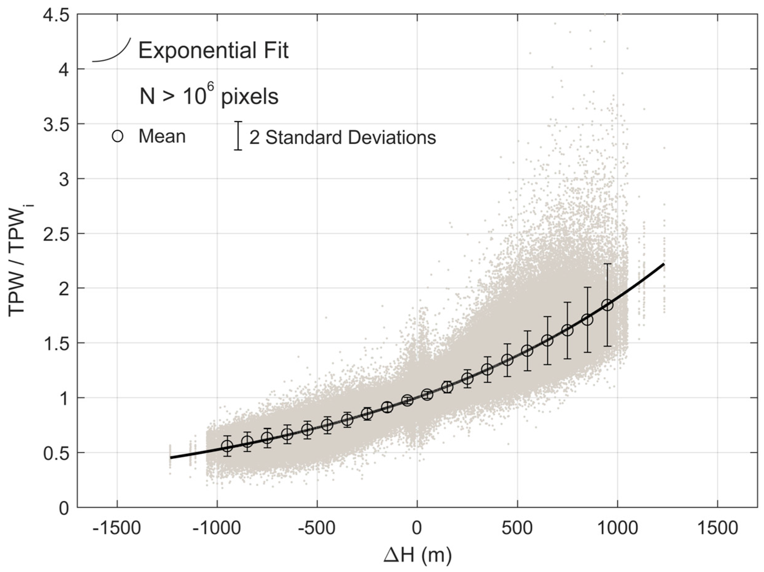
• The exponential parametrization of Total Column Water Vapor. Assuming hydrostatic equilibrium, which is a good approximation for the vertical dependence of the pressure field in the real atmosphere, TPW decreases exponentially with height, where the rate of decay depends on the temperature lapse rate. As such, we tested a parametrization based on the exponential decrease of TPW with altitude [32,33], i.e.,

  $${\mathrm{TPW}}_1={\mathrm{TPW}}_0\exp \left(\frac{{\mathrm{H}}_0-{\mathrm{H}}_1}{\mathsf{\alpha }}\right)$$

  (4)

  where ${\mathrm{TPW}}_1$ and ${\mathrm{TPW}}_0$ are the estimated and reference TPW, respectively. ${\mathrm{H}}_1$ and ${\mathrm{H}}_0$ are the high and coarse resolution altitude, respectively. The scale parameter α is estimated by linear regression using COSMO fields of height and TPW for all grid-points and for all data considered in this study. For each COSMO grid point and observation, we considered the values of height and of TPW over each grid point and the surrounding eight neighbors. Differences in H and ratios in TPW were then computed between surrounding neighbors and the central grid point (Figure 4). Taking into account COSMO spatial resolution of about 2 km, the rationale is that for the area delimited by the eight neighbors, changes in TPW are mainly driven by differences in topography, while the thermodynamic properties of the atmospheric profile are maintained. The value of parameter $\mathsf{\alpha }$ is then estimated by linear regression performed between differences in H and the natural logarithm of the ratios in TPW. The obtained estimate for parameter α was 1547 m, i.e., TPW decreased by a factor of e when surface elevation increased by 1547 m.
• The Level reduction, which consists of using the surface pressure from COSMO and then, by linear interpolation, truncating the ERA-Int profile at that COSMO pressure level. This method is required for radiative transfer based LST retrieval algorithms (that use water vapor and temperature profiles as input). The method may also be used for statistically based algorithms with the drawback of introducing more variables to the models (thermodynamic profiles, where only TPW is required).

We will restrict its use to cases where surface height is underestimated, as these correspond to the most critical cases where deviations of ERA-Int surface from actual orography may reach 1000 m or more (Figure 2 and Figure 3).

3. Results

3.1. Difference between ERA-Int and COSMO TPW

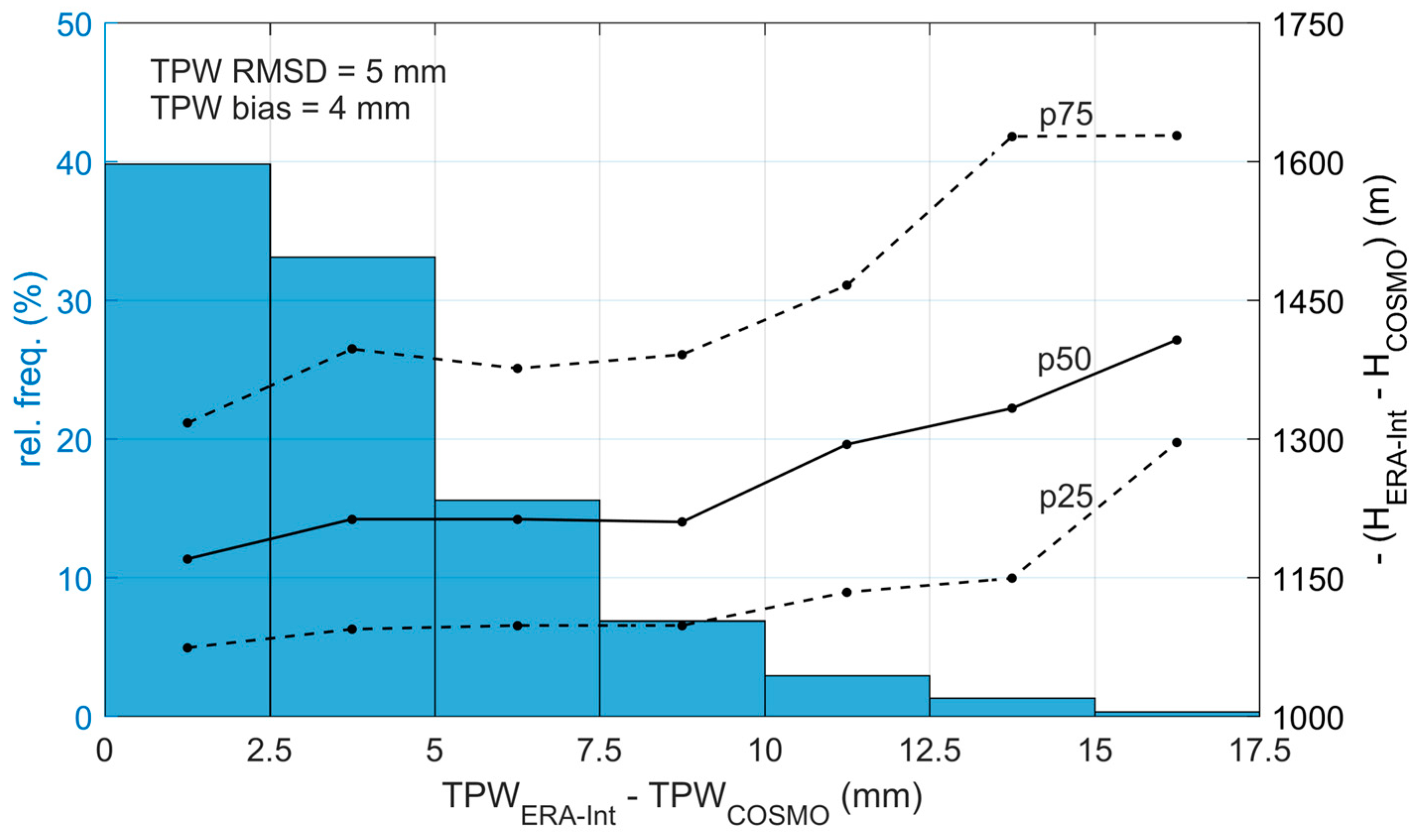
The comparison between ERA-Int TPW and COSMO reference TPW is shown in Figure 5 for grid points with altitude differences (COSMO minus ERA-Int) greater than 1000 m. Differences in TPW reach a maximum of 17.2 mm and present an average of 4 mm and root mean square difference (RMSD) of 5 mm. For each bin of the histogram (Figure 5), the median (black solid line), 25th, and 75th percentiles of height differences between ERA-Int and the reference COSMO indicate that the differences of height tend to be larger with the increase in the departures of ERA-Int TPW from reference.

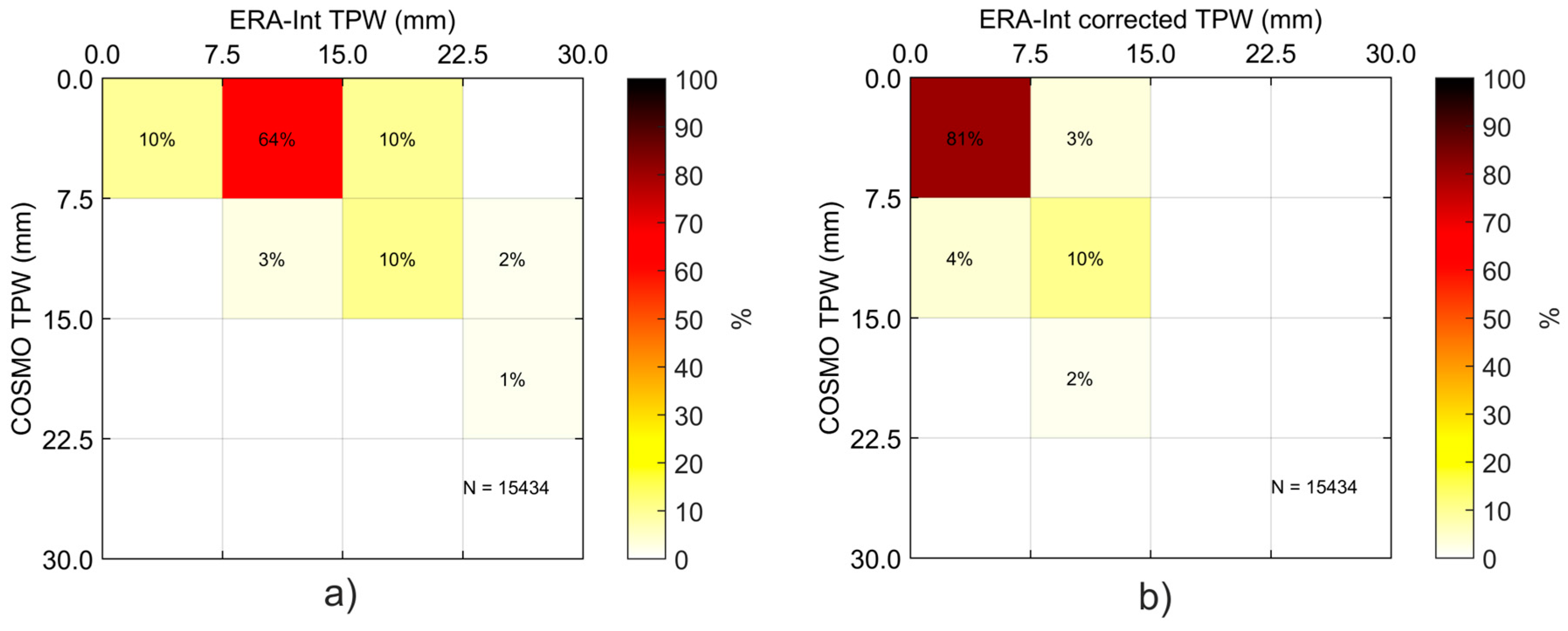
Figure 6 shows the agreement between TPW classes determined by ERA-Int and COSMO profiles, plotting the percentage of cases that fall in different pairs of ERA-Int/COSMO TPW classes for the period between April and September. The selected period corresponds to the season where (clear sky) TPW is most variable, when the atmosphere is warmer, and, therefore, able to hold larger water vapor contents. When ERA-Int is compared with COSMO without any orographic correction (Figure 5a), only 13% (i.e., 10% + 3% along the diagonal) of the total amount of grid-points are in the same TPW class, i.e., about 87% of ERA-Int profiles (i.e., the total of off-diagonal cells) are in the wrong TPW class. Furthermore, about 75% of the points miss by one class and 12% by two classes (Figure 6a). If the exponential parametrization (Equation (4)) is applied (Figure 6b), then the fraction of correct hits rises from 13% to 91% (i.e., 81% + 10% along the diagonal). The remaining 9% differ by one class.

3.2. Sensitivity Analysis

Since, to our knowledge, there are no LST validation in situ stations at high altitudes, a proper validation study of the proposed corrections is still not possible. Instead, a sensitivity study was performed in which LST was retrieved using each of the three above mentioned algorithms using COSMO profiles (for PMW) and COSMO TPW (for GSW and SMW). These LSTs were considered as the reference. Next, LST was retrieved for the same grid-points under the same conditions, but with ERA-Int profiles/TPW. The same procedure was repeated using corrected ERA-Int profiles/TPW. The exponential parametrization method (Equation (4)) was applied to get corrected TPW fields for GSW and SMW, while the level reduction method was applied to adjust the profiles used by the PMW. The RMSD was computed to compare LST retrieved with ERA-Int profiles and the reference LST (retrieved with COSMO profiles). The same procedure was applied when comparing the corrected LST.

Table 1. Land surface temperature (LST) root mean square difference (RMSD) (K) when comparing LST derived with COSMO profiles (reference) and LST derived with ERA-Int original profiles (Orig) and ERA-Int corrected with the different methods (Corr), for a physical mono-window (PMW) (a), statistical mono-window (SMW) (b), and generalized split-windows (GSW) (c). N represents the number of profiles in a determined class of altitude difference and season. The seasons are extended winter (November–March) and extended summer (April–September).

LST (K) (RMSD)	1000 < $\mathbf{\Delta }\mathbf{H}$ < 1250			1250 < $\mathbf{\Delta }\mathbf{H}$ < 1500			1500 < $\mathbf{\Delta }\mathbf{H}$ < 1750			$\mathbf{\Delta }\mathbf{H}$ > 1750
	Orig	Corr	N	Orig	Corr	N	Orig	Corr	N	Orig	Corr	N
	(a) PMW
November–March	0.3	0.0	16,544	0.4	0.0	7230	0.5	0.0	2762	0.6	0.0	1126
April–September	1.0	0.2	9091	1.2	0.2	4132	1.3	0.1	1582	1.8	0.1	629
	(b) SMW
November–March	0.1	0.0	16,544	0.0	0.0	7230	0.0	0.0	2762	0.0	0.0	1126
April–September	0.5	0.2	9091	0.5	0.2	4132	0.5	0.1	1582	0.4	0.0	629
	(c) GSW
November–March	0.1	0.0	16,544	0.0	0.0	7230	0.0	0.0	2762	0.0	0.0	1126
April–September	0.4	0.1	9091	0.4	0.1	4132	0.4	0.1	1582	0.3	0.0	629

shows LST RMSD per season—November to March and April to September which, for simplicity, we will call extended winter and extended summer, respectively—and per difference in ERA-Int and COSMO surface height, for PMW, SMW, and GSW.

As shown in Table 1(a), the RMSD obtained for PMW forced with ERA-Int increased with elevation, regardless of the season. RMSD ranged between 0.3 K (extended winter, for altitude differences between 1000 and 1250 m) and 1.8 K (extended summer, for altitude differences greater than 1750 m). When the level reduction orographic correction was applied, RMSD decreased significantly, with new values ranging between 0 K (several cases) and 0.2 K (extended summer, for altitude differences between 1000 m and 1250 m and between 1250 m and 1500 m). Furthermore, the highest RMSD of 1.8 K in extended summer 2014, for altitudes greater than 1750 m, decreased to 0.1 K.

The RMSD estimated for SMW LST are shown in Table 1(b). Here, the results are not as striking as for the PMW, where LST had a strong dependence on the season but not on the elevation differences. RMSD ranged between 0 K (in several cases) and 0.5 K in the extended summer months, a period when TPW values in the clear-sky atmosphere are usually larger. When the exponential parametrization orographic correction was applied, RMSD also decreased, with a maximum gain of 0.4 K.

Finally, as shown in Table 1(c), the GSW LST RMSD present the same behavior as the SMW, showing a higher dependence on month of the year than on altitude differences. Here, RMSD ranged between 0 K (in several cases) and 0.4 K (extended summer, for altitude differences between 1000 m and 1750 m). Again, the most critical cases seemed to occur during the warmer period of the year, when the TPW tends to be higher under cloud-free conditions.

These results indicate that PMW is much more sensitive to water vapor than SMW and GSW. This is because PMW requires the whole water vapor profile rather than column integrated values, and for small changes in the water vapor profile, the retrieved LST value will also change. Conversely, both SMW and GSW depend on classes of TPW, which means that a small change (or even a substantial change, considering that the TPW classes are generally broad) in water vapor may have no effect on LST. Furthermore, GSW is less sensitive to the TPW input than SMW, as the differences in the two adjacent split-window channels are themselves sensitive to the actual water content in the atmosphere (e.g., [19,20,21]).

4. Discussion

There is growing evidence that the rate of warming is amplified with elevation [16]. Air temperature observations at ground stations are essential to study elevation-dependent warming, but many high-altitude areas are still heavily under-sampled [17]. To overcome those limitations, spatially-continuous remotely-sensed land surface temperature (LST) climate data from satellites could be used for elevation dependent warming studies [16,18]. This study addresses systematic errors that can be present in satellite-based LST retrievals at high-altitudes and proposes methods to correct for those errors.

Long-term satellite-based LST retrieval algorithms from geostationary satellite sensors rely on reanalyses data (such as ERA-Int) with a relatively coarse horizontal resolution to estimate the atmospheric water vapor content. This implies a rather poor representation of small scale orographic features. In particular, reanalyzed water vapor fields can significantly depart from real values for pixels in mountainous regions. For the Alpine region investigated in this study, these differences reach a maximum of 17.2 mm.

The impact of the different water vapor estimates in three different LST retrieval schemes (the SMW, the GSW, and the PMW) was assessed. In the case of SMW and GSW, only vertically integrated water vapor affects the retrieval, as these models are calibrated in classes of TPW (in steps of 7.5 mm). Errors in TPW translate into the selection of the wrong class, i.e., the wrong set of model coefficients will be used, which allows a margin of TPW uncertainty within each correct class.

In terms of class hits (Figure 6), ERA-Int profiles miss the TPW class in 87% of the cases, where 75% of these misses reflect a deviation of one class and 12% of two classes. It was shown that the exponential parametrization orographic correction method dramatically improves the amount of ERA-Int profiles within the correct class (91%). These results correspond to the cases where ERA-Int orography field exceeds the higher resolution orography in more than 1000 m.

Results presented in Table 1 show that the radiative transfer based algorithm (PMW) is much more sensitive to water vapor when the original ERA-Int profiles are used. The PMW takes the full ERA-Int profiles as one of its inputs, i.e., the atmospheric radiances and transmissivity will be affected by errors in the profile. Furthermore, for the thermal window channels used for LST estimation, radiative transfer is particularly sensitive to the lower levels in the atmosphere where most water vapor content lies. Therefore, when inverting the radiative transfer equation and the calibrated Planck function, LST will be affected even with a relatively small change in the humidity profile.

This work mainly consists of an LST sensitivity study to water vapor errors related to the misrepresentation of the surface orography associated to each atmospheric profile. For that purpose, we compare LST retrievals using water vapor inputs with different spatial resolutions in the Alpine region. We show that RMSD up to 1.8 K may arise in LST retrievals (Table 1) over pixels where the profile surface height deviates by 1000 m or more from a reference orography. We also show that the largest height deviations in models occur for high elevations, where TPW is systematically overestimated and, therefore, will be a source of systematic errors in LST retrievals. We further show that this may be overcome by an adequate adjustment of reanalysis profiles and/or total column water vapor to the geographic elevation. When using the level reduction method, the highest RMSD of 1.8 K in extended summer 2014, for altitudes greater than 1750 m, decreased to 0.1 K (Table 1).

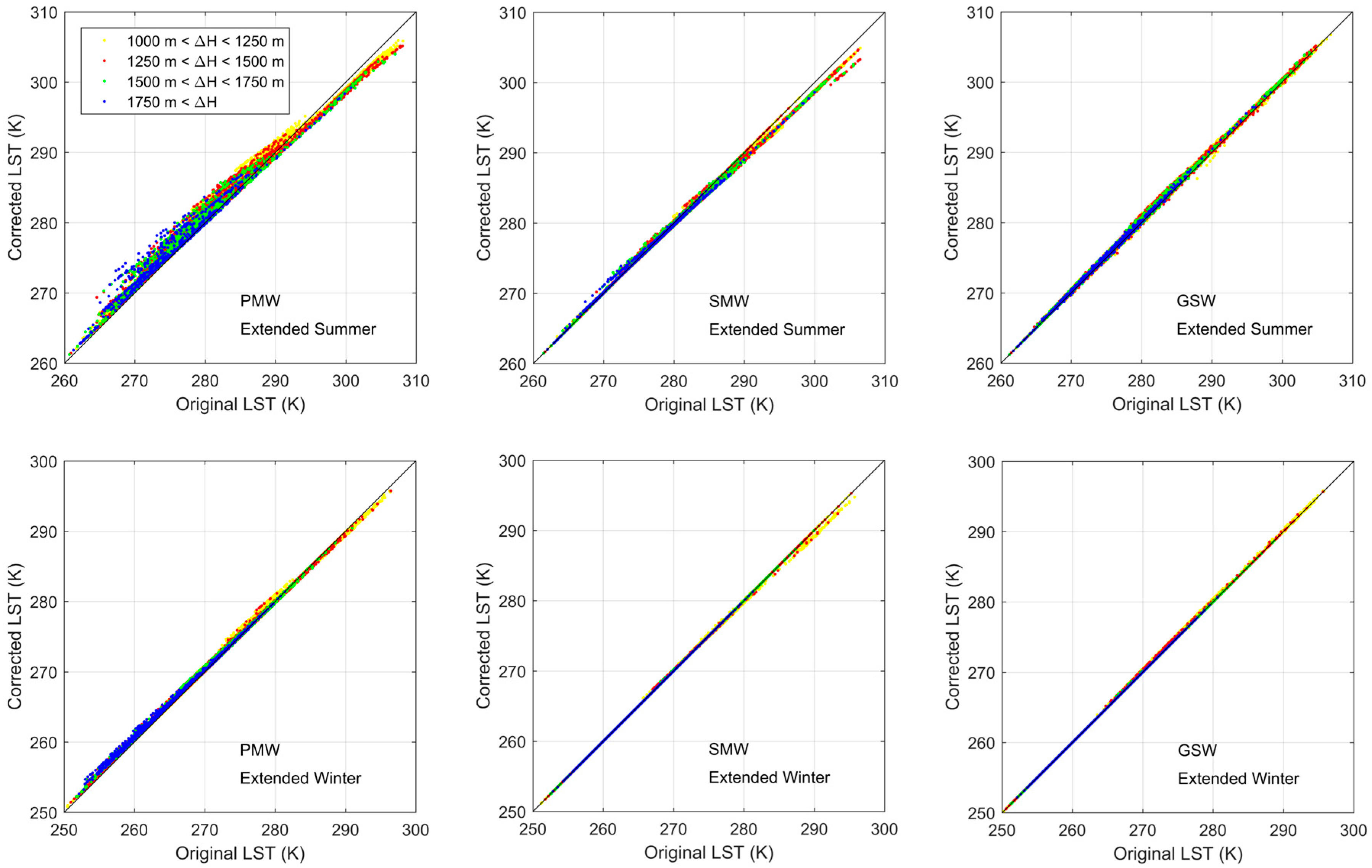
A deeper insight into the impact of height deviations on LST estimates for three LST retrieval algorithms is provided by scatterplots of corrected versus original values of LST for the different classes of ΔH and for extended summer and winter (Figure 7). The above mentioned larger sensitivity of PMW (followed by SMW) to water vapor translates into the deviations from the 1:1 line which increase from right to left in the panels of the figure. As also discussed, deviations are larger during the extended summer than during the extended winter, reflecting the larger amounts of water vapor in the former season than in the latter. It is worth noting that corrections do not present a systematic character, tending to decrease (increase) towards lower (higher) LST values. This implies that, on average, corrections will have lower values. Finally, it is worth noting that biases in the corrections are strongly conditioned by the value of LST, a major issue that must be taken into account when LST data are used for climatological purposes, namely when building up CDRs.

An ideal validation of results would require data from in situ high altitude LST dedicated stations, which were not available in the course of this study. Furthermore, due to the large footprint of MSG/SEVIRI pixel (3–5 km), ideal conditions (as those provided by an LST dedicated station at high altitude in a homogeneous region at the sensor spatial resolution) would be very difficult to achieve.

5. Conclusions

Studies focusing on elevation dependent warming related to climate change have been facing difficulties related to the scarceness of air temperature in-situ observations over mountainous regions. The current availability of long-term time series of spatially continuous data of remotely-sensed Land Surface Temperature (LST) appears as a valuable means to overcome this problem. One example of such a database is the one being produced by CM SAF and LSA SAF. However, the algorithms used to retrieve LST depend on reanalyzed water vapor profiles defined in a grid associated to a smoothed orography, which leads to misestimations in the water vapor profile.

Two orographic correction methodologies were developed aiming at improving LST retrievals by correcting the water vapor profile and/or the total precipitable water estimations. Improvements in the LST retrieval vary depending on the method used but may reach 1.7 K (RMSD), an extremely large discrepancy for climatological applications.

Given the lack of in-situ LST stations in high altitude regions, a direct comparison against ground measurements was not possible at this stage. The relatively large footprint of the MSG/SEVIRI pixel makes the task difficult to achieve. Nevertheless, LST products derived from MSG/SEVIRI or other sensors would certainly benefit from field campaigns in high-elevation regions, and are needed to close an important gap in satellite product validation.

This study was performed over the Alpine region, which despite being the highest mountain range in Europe is not the highest mountain range encompassed in the MSG-disk, and is far from being the highest mountain range in the world. An example is Mount Kilimanjaro in eastern Africa, which is also within the MSG-disk. This mountain reaches an altitude of about 5900 m, while the ERA-Int orographic field has a maximum of 2115 m. Differences here may reach 3800 m, a value well above those covered in this study since the maximum difference in the Alps only goes as high as about as 2500 m.

LST estimates in high elevation regions may be affected by other sources of error, namely due to the high spatial (and temporal) variability of surface emissivity associated to the changes in landcover and snow/ice with height. Getting a highly detailed emissivity map over mountain regions is challenging, and should be covered in future works.

References

- Crago, R.D.; Qualls, R.J. Use of land surface temperature to estimate surface energy fluxes: Contributions of Wilfried Brutsaert and collaborators. Water Resour. Res. 2014, 50, 3396–3408. [Google Scholar] [CrossRef]
- Trigo, I.F.; Viterbo, P.; Trigo, I.F.; Viterbo, P. Clear-sky window channel radiances: A comparison between observations and the ECMWF model. J. Appl. Meteorol. 2003, 42, 1463–1479. [Google Scholar] [CrossRef]
- Trigo, I.F.; Boussetta, S.; Viterbo, P.; Balsamo, G.; Beljaars, A.; Sandu, I. Comparison of model land skin temperature with remotely sensed estimates and assessment of surface-atmosphere coupling. J. Geophys. Res. Atmos. 2015, 120, 12096–12111. [Google Scholar] [CrossRef]
- Ghent, D.; Kaduk, J.; Remedios, J.; Ardö, J.; Balzter, H. Assimilation of land surface temperature into the land surface model JULES with an ensemble Kalman filter. J. Geophys. Res. 2010, 115, D19112. [Google Scholar] [CrossRef]
- Reichle, R.H.; Kumar, S.V.; Mahanama, S.P.P.; Koster, R.D.; Liu, Q.; Reichle, R.H.; Kumar, S.V.; Mahanama, S.P.P.; Koster, R.D.; Liu, Q. Assimilation of satellite-derived skin temperature observations into land surface models. J. Hydrometeorol. 2010, 11, 1103–1122. [Google Scholar] [CrossRef]
- Caparrini, F.; Castelli, F.; Entekhabi, D. Variational estimation of soil and vegetation turbulent transfer and heat flux parameters from sequences of multisensor imagery. Water Resour. Res. 2004, 40, 1–15. [Google Scholar] [CrossRef]
- Kalman, R.E. A new approach to linear filtering and prediction problems. J. Basic Eng. 1960, 82, 35–45. [Google Scholar] [CrossRef]
- Kalman, R.E.; Bucy, R.S. New results in linear filtering and prediction theory. J. Basic Eng. 1961, 83, 95–107. [Google Scholar] [CrossRef]
- Kustas, W.P.; Norman, J.M. Use of remote sensing for evapotranspiration monitoring over land surfaces. Hydrol. Sci. J. 1996, 41, 495–516. [Google Scholar] [CrossRef]
- Wan, Z.; Wang, P.; Li, X. Using MODIS land surface temperature and normalized difference vegetation index products for monitoring drought in the southern Great Plains, USA. Int. J. Remote Sens. 2004, 25, 61–72. [Google Scholar] [CrossRef]
- Duguay-Tetzlaff, A.; Bento, V.; Göttsche, F.; Stöckli, R.; Martins, J.; Trigo, I.; Olesen, F.; Bojanowski, J.; da Camara, C.; Kunz, H. Meteosat land surface temperature climate data record: Achievable accuracy and potential uncertainties. Remote Sens. 2015, 7, 13139–13156. [Google Scholar] [CrossRef]
- Siemann, A.L.; Coccia, G.; Pan, M.; Wood, E.F. Development and analysis of a long-term, global, terrestrial land surface temperature dataset based on HIRS satellite retrievals. J. Clim. 2016, 29, 3589–3606. [Google Scholar] [CrossRef]
- Dee, D.P.; Uppala, S.M.; Simmons, A.J.; Berrisford, P.; Poli, P.; Kobayashi, S.; Andrae, U.; Balmaseda, M.A.; Balsamo, G.; Bauer, P.; et al. The ERA-Interim reanalysis: Configuration and performance of the data assimilation system. Q. J. R. Meteorol. Soc. 2011, 137, 553–597. [Google Scholar] [CrossRef]
- Good, E. Daily minimum and maximum surface air temperatures from geostationary satellite data. J. Geophys. Res. Atmos. 2015, 120, 2306–2324. [Google Scholar] [CrossRef]
- Oyler, J.W.; Dobrowski, S.Z.; Holden, Z.A.; Running, S.W.; Oyler, J.W.; Dobrowski, S.Z.; Holden, Z.A.; Running, S.W. Remotely sensed land skin temperature as a spatial predictor of air temperature across the conterminous United States. J. Appl. Meteorol. Climatol. 2016, 55, 1441–1457. [Google Scholar] [CrossRef]
- Mountain Research Initiative EDW Working Group. Elevation-dependent warming in mountain regions of the world. Nat. Clim. Chang. 2015, 5, 424–430. [Google Scholar] [Green Version]
- Lawrimore, J.H.; Menne, M.J.; Gleason, B.E.; Williams, C.N.; Wuertz, D.B.; Vose, R.S.; Rennie, J. An overview of the Global Historical Climatology Network monthly mean temperature data set, version 3. J. Geophys. Res. Atmos. 2011, 116, D19121. [Google Scholar] [CrossRef]
- Qin, J.; Yang, K.; Liang, S.; Guo, X. The altitudinal dependence of recent rapid warming over the Tibetan Plateau. Clim. Chang. 2009, 97, 321–327. [Google Scholar] [CrossRef]
- Li, Z.-L.; Tang, B.-H.; Wu, H.; Ren, H.; Yan, G.; Wan, Z.; Trigo, I.F.; Sobrino, J.A. Satellite-derived land surface temperature: Current status and perspectives. Remote Sens. Environ. 2013, 131, 14–37. [Google Scholar] [CrossRef]
- Masiello, G.; Serio, C.; De Feis, I.; Amoroso, M.; Venafra, S.; Trigo, I.F.; Watts, P. Kalman filter physical retrieval of surface emissivity and temperature from geostationary infrared radiances. Atmos. Meas. Tech. 2013, 6, 3613–3634. [Google Scholar] [CrossRef]
- Masiello, G.; Serio, C.; Venafra, S.; Liuzzi, G.; Göttsche, F.; Trigo, I.F.; Watts, P. Kalman filter physical retrieval of surface emissivity and temperature from SEVIRI infrared channels: A validation and inter-comparison study. Atmos. Meas. Tech. 2015, 8, 2981–2997. [Google Scholar] [CrossRef]
- Freitas, S.C.; Trigo, I.F.; Bioucas-Dias, J.M.; Göttsche, F.M. Quantifying the uncertainty of land surface temperature retrievals from SEVIRI/Meteosat. IEEE Trans. Geosci. Remote Sens. 2010, 48, 523–534. [Google Scholar] [CrossRef]
- Derrien, M.; Gléau, H. MSG/SEVIRI cloud mask and type from SAFNWC. Int. J. Remote Sens. 2005, 21, 4707–4732. [Google Scholar] [CrossRef]
- Trigo, I.F.; Dacamara, C.C.; Viterbo, P.; Roujean, J.-L.; Olesen, F.; Barroso, C.; Camacho-de-Coca, F.; Carrer, D.; Freitas, S.C.; García-Haro, J.; et al. The satellite application facility for land surface analysis. Int. J. Remote Sens. 2011, 32, 2725–2744. [Google Scholar] [CrossRef]
- Baldauf, M.; Seifert, A.; Förstner, J.; Majewski, D.; Raschendorfer, M. Operational convective-scale numerical weather prediction with the COSMO model: Description and sensitivities. Mon. Weather Rev. 2011, 139, 3887–3905. [Google Scholar] [CrossRef]
- Wan, Z.; Dozier, J. A generalized split-window algorithm for retrieving land-surface temperature from space. IEEE Trans. Geosci. Remote Sens. 1996, 34, 892–905. [Google Scholar]
- Trigo, I.F.; Monteiro, I.T.; Olesen, F.; Kabsch, E. An assessment of remotely sensed land surface temperature. J. Geophys. Res. 2008, 113, D17108. [Google Scholar] [CrossRef]
- Trigo, I.F.; Peres, L.F.; DaCamara, C.C.; Freitas, S.C. Thermal land surface emissivity retrieved from SEVIRI/Meteosat. IEEE Trans. Geosci. Remote Sens. 2008, 46, 307–315. [Google Scholar] [CrossRef]
- Martins, J.P.A.; Trigo, I.F.; Bento, V.A.; da Camara, C. A Physically constrained calibration database for land surface temperature using infrared retrieval algorithms. Remote Sens. 2016, 8, 808. [Google Scholar] [CrossRef]
- Yu, X.; Guo, X.; Wu, Z. Land surface temperature retrieval from Landsat 8 TIRS—Comparison between radiative transfer equation-based method, split window algorithm and single channel method. Remote Sens. 2014, 6, 9829–9852. [Google Scholar] [CrossRef]
- Matricardi, M.; Chevallier, F.; Tjemkes, S. An improved general fast radiative transfer model for the assimilation of radiance observations. ECMWF Tech. Memo. 2001, 345, 153–173. [Google Scholar] [CrossRef]
- Basili, P.; Bonafoni, S.; Mattioli, V.; Ciotti, P.; Pierdicca, N. Mapping the atmospheric water vapor by integrating microwave radiometer and GPS measurements. IEEE Trans. Geosci. Remote Sens. 2004, 42, 1657–1665. [Google Scholar] [CrossRef]
- Morland, J.; Mätzler, C. Spatial interpolation of GPS integrated water vapour measurements made in the Swiss Alps. Meteorol. Appl. 2007, 14, 15–26. [Google Scholar] [CrossRef]
© 2017 by the authors; licensee MDPI, Basel, Switzerland. This article is an open access article distributed under the terms and conditions of the Creative Commons Attribution (CC-BY) license (http://creativecommons.org/licenses/by/4.0/).