IceMap250—Automatic 250 m Sea Ice Extent Mapping Using MODIS Data

Abstract

The sea ice cover in the North evolves at a rapid rate. To adequately monitor this evolution, tools with high temporal and spatial resolution are needed. This paper presents IceMap250, an automatic sea ice extent mapping algorithm using MODIS reflective/emissive bands. Hybrid cloud-masking using both the MOD35 mask and a visibility mask, combined with downscaling of Bands 3–7 to 250 m, are utilized to delineate sea ice extent using a decision tree approach. IceMap250 was tested on scenes from the freeze-up, stable cover, and melt seasons in the Hudson Bay complex, in Northeastern Canada. IceMap250 first product is a daily composite sea ice presence map at 250 m. Validation based on comparisons with photo-interpreted ground-truth show the ability of the algorithm to achieve high classification accuracy, with kappa values systematically over 90%. IceMap250 second product is a weekly clear sky map that provides a synthesis of 7 days of daily composite maps. This map, produced using a majority filter, makes the sea ice presence map even more accurate by filtering out the effects of isolated classification errors. The synthesis maps show spatial consistency through time when compared to passive microwave and national ice services maps.

1. Introduction

The prospect of increased economic activity in the Arctic, accompanied by increased marine traffic, suggests that the need for sea ice information will increase in the future. Marine engineers will need more spatially and temporally precise data in order to monitor sea ice behavior around marine infrastructure, offshore platforms, and ships [1]. Ecologists will also need access to more sea ice data to understand the impact of climate change on species habitats. More precise and frequently available data would also help climatologists to get a clearer look at the ice–albedo feedback.

Remote sensing images have been used for decades to generate numerous sea ice monitoring products. Depending on the desired scientific or operational application, remote sensing platforms and sensors producing passive microwave (PM) [2,3,4,5], synthetic aperture radar (SAR) [6,7,8], or visible (VIS) and thermal infrared (TIR) [9,10,11] imagery can be utilized.

The major users of remote sensing data for ice survey and mapping purposes are the national ice services, such as the Canadian Ice Service, the National Ice Center (USA), the Norwegian Meteorological Institute and the Danish Meteorological Institute. These services use multiple sources of imagery to produce added-value datasets for many end users, but mostly for navigation purposes [12]. Most datasets are produced on either a daily, weekly, or fortnightly basis. For example, the analysts of the Canadian Ice Service use a combination of in-situ observations and satellite datasets to synthesize and integrate ice information into a single ice concentration or stage of development map [13], utilizing the “egg code“ and following the official World Meteorological Organization color codes. SAR imagery is the backbone data used by ice services as it is characterized by a high spatial resolution, an all-weather capability and a complete independence to daylight. The highest resolution used to create the maps is about 50 m, corresponding to the resolution of RADARSAT data in ScanSAR mode. The sea ice maps provided by national ice services provide high-quality information, but nevertheless do not provide fine resolution details about ice extent on a daily basis, even if their main input is high-resolution SAR data [12].

Passive microwave sensors such as SMMR, SSM/I, SSMIS, AMSR/E, and AMSR2, have as main advantage that they offer data with daily global coverage; their main disadvantage being that they have a coarse spatial resolution. Many algorithms were developed to retrieve sea ice concentrations from passive microwave observations, as presented by Ivanova et al. [2]. From these algorithms, some use higher frequency bands to achieve finer grid resolution, such as the ARTIST Sea Ice Algorithm (ASI) from Kaleschke et al. [14] and the SEA LION algorithm from Kern [15] at 12.5 km for use with SSM/I, the ASI applied to AMSR-E from Spreen et al. [5] achieving a 6.25 km grid resolution and another application of the ASI to AMSR2, by Beitsch et al. [16], achieving a 3.125 km grid resolution. It is important to note that the higher the frequency used in passive microwave, the more the signal is subject to weather influences. Most ice concentration (SIC) and hence sea ice extent time series are based on passive microwave data obtained at the lower frequency channels as these are almost not influenced by clouds and allow a daily temporal resolution. The convention used by many authors is that ice is computed when concentrations >15% [12], though algorithms can detect sea ice concentrations down to 0%. Near coastlines, the passive microwave datasets are subject to land contamination, meaning that the received signal is a mix of both land and water signals, due to the large footprint. If not assessed the land contamination tends to cause over-estimation of the sea ice extent [17].

SAR sensors, such as Radarsat-2 and Sentinel-1A, are used to monitor sea ice at a fine spatial resolution depending on the selected acquisition mode (5 to 100 m). The main advantage of SAR is that it is independent of daylight and weather conditions. This explains why SAR is frequently used by national ice services as the main source of information in their operational map production. However, although SAR shows great potential for use by sea ice analysts, there is no mature operational quantitative algorithm for automatic ice concentration estimation [12].

Visible and TIR imagery are used to monitor the limit of the ice also called the ice edge. This information is crucial for calculating the extent of the ice cover [12]. The visible sensors usually achieve a high resolution that reduces land contamination and enables finer estimation of ice presence in narrow passages and archipelago regions. Although highly affected by cloud cover and daylight conditions [18], visible and TIR data are often used to assess the quality and accuracy of SAR and passive microwave maps [19,20,21,22]. Different sea ice mapping approaches are used with optical sensors such as MODIS [9,23,24,25] and VIIRS [26].

All of the previously presented approaches to sea ice mapping are complementary and can be used in synergy to analyze and understand ice cover spatiotemporal changes. To complement the offer in data and to answer the needs in terms of high spatial and temporal resolutions, this paper proposes a new ice mapping algorithm, called IceMap250, based on the use of MODIS multispectral spectroradiometers. MODIS shows great potential, providing a spatial resolution of 250–1000 m combined with daily global coverage. The automated process to map sea ice presence is inspired by the original IceMap algorithm [23] but including three improvements: (1) a finer, 250 m spatial resolution made possible by using the Canadian Centre for Remote Sensing [27] downscaling algorithm; (2) use of a hybrid cloud-masking approach; (3) use of a more efficient spectral ratio to detect sea ice (the NDSII–2 index) [28]. The proposed algorithm provides improved accuracy for sea ice mapping due to finer spatial resolution and an improved set of decision thresholds. These improvements will help monitor sea ice at a finer scale and provide valuable information at a 250 m spatial resolution in a near real-time frame.

2. Materials and Methods

2.1. Study Area

The region selected to test IceMap250 is the Hudson Bay Complex (Figure 1), located in Northeastern Canada. This region is considered the largest inland sea in the world, covering an area of 1,230,000 km².

The ice regime varies in the different parts of the Hudson Bay Complex [29]. In James Bay, the southernmost part of the study area, complete freeze-up is usually achieved in December and complete melting is usually completed in July. In Hudson Bay, freeze-up begins between early October and late November and melting occurs between mid-July and early September. In Hudson Strait, ice usually appears late September and melt usually completes in August. Finally, in Foxe Basin, the northernmost part of the study area, complete clearing of the sea ice cover does not occur every year.

2.2. Data Used in IceMap250

2.2.1. MODIS Sensors and Datasets

MODIS-Terra was launched on 18 December 1999, started acquiring images on 24 February 2000, and is still acquiring images today. With a 2330 km view swath, the sensor captures information on every point of the planet every 1 or 2 days, with 36 spectral bands ranging from visible to thermal infrared (0.45 to 14.4 μm) at a spatial resolution ranging from 250 to 1000 m. The MODIS-Terra platform has a sun-synchronous orbit with a descending node at 10:30 UTC and is on a 16-day repeat cycle. MODIS-Aqua was launched on 4 May 2002 and offers the same capabilities and technical properties as Terra. It is important to note that 70% of the detectors for Band 6 (1.64 μm) failed shortly after launch and that Aqua products use Band 7 (2.13 μm) instead of Band 6 in their computations [30]. The Aqua satellite has an ascending node at 13:30 UTC and is also on a 16-day repeat cycle.

Bands 1 to 7 are used in the IceMap250 processing (

Table 1. MODIS Bands 1 to 7 spatial and spectral characteristics.

Band Number	Grid Resolution (m)	Bandwidth (μm)	Part of Spectrum
1	250	0.62–0.67	VIS (red)
2	250	0.841–0.876	NIR
3	500	0.459–0.479	VIS (blue)
4	500	0.545–0.565	VIS (green)
5	500	1.230–1.250	NIR
6	500	1.628–1.652	SWIR
7	500	2.105–2.155	SWIR

).

Data from both MODIS sensors are available for free from the Level 1 and Atmosphere Archive and Distribution System (LAADS), which is updated every day. The IceMap250 algorithm uses data from five different MODIS collection 6 products. The MODIS-Aqua products are the same, but the prefix of the file name is MYD instead of MOD.

• MOD021KM: MODIS-Terra 1 km data;
• MOD02HKM: MODIS-Terra 500 m data;
• MOD02QKM: MODIS-Terra 250 m data;
• MOD03: MODIS-Terra geolocation product;
• MOD35_L2: MODIS-Terra cloud mask product.

MODIS-Terra and Aqua capture scenes of the Hudson Bay Complex at different times depending on their position in their respective cycles and the images are acquired during MODIS overpasses in order to have sufficient daylight conditions. Acquisitions are made on two following descending tracks between 14:45 and 18:30 UTC, meaning between 9:45 and 13:30 EST (local time) for Terra, and on two following ascending tracks between 15:45 and 19:30 UTC, meaning between 10:45 and 14:30 EST (local time) for Aqua. Datasets in these time ranges are acquired automatically according to the satellite orbit cycle (16 days) and processed with the IceMap250 algorithm on reception of the data files. Alternate overpasses for both Terra (ascending) and Aqua (descending) are during the night and therefore are not used in IceMap250 as it uses only reflective bands and no thermal information in its decision thresholds, in contrast to the original algorithm.

Algorithm validation scenes were selected to cover the three important periods of the sea ice regime during the year: freeze-up, stable cover, and melt. Continuous five-day segments of each period were selected in order to assess the consistency of the algorithm. The ice regime periods were defined based on the 1981–2010 Canadian Ice Service Hudson Bay regional climatology [29]. Selected test scenes are:

• For the stable period from 10 February 2016 to 20 February 2016 (Day of year 41 to 51);
• For the melt period from 13 June 2013 to 23 June 2013 (Day of year 165 to 175);
• For the freeze-up period from 1 December 2015 to 11 December 2015 (Day of year 335 to 345).

The periods were selected to embrace a wide range of conditions, extending from a very cloudy freeze-up scene to a perfectly clear sky summer melt scene.

2.2.2. Land Mask

Land masking is achieved using a coastline vector file obtained from the Natural Earth website [31]. This coastline vector, based on the World Data Bank II (a.k.a. CIA data bank), has an estimated resolution of 500 m [32].

2.3. Spectral Behavior of Sea Ice in the Visible Spectrum

The differences in albedo and surface temperature of ice and water can be used to distinguish the two in respectively the visible and the near-infrared part of the spectrum [12]. Sea ice, which is in most cases snow-covered [33], exhibits fairly constant reflectance whatever the solar zenith angle (the incident solar beam angle), except when the sensor zenith angle (reflection angle toward the sensor) is equal to the zenith angle of the direct solar beam, meaning that the solar beam is reflected in a specular way, generating a peak in reflectance [34]. The more the solar zenith angle increases (the sun gets closer to the horizon), the more specular reflection increases, with the reflection being greater for smooth surfaces such as blue ice or an open melt pond and smaller for rough surfaces such as snow [35]. In terms of wavelength dependence, snow-covered sea ice reflectance decreases with increasing wavelengths in the 450–950 nm part of the spectrum (Figure 2).

According to Barber et al. [36], who studied snow grain sizes on first-year sea ice in Lancaster Sound in Nunavut, the snow grain sizes measured varied from 0.4 to 2.5 mm (400–2500 μm). The impact of the snow grain size is varying depending on the wavelength. In the visible part, the impact of grain size is small when compared to the impact snow grain size has on the near infrared signal. However, ice is not snow covered all the time and follows a certain characteristic path during its formation, well described by Perovich and Polashenski [33]. During the freeze up, new ice forms up, in the form of nilas and grease ice, without any snow cover. These forms of ice have slightly higher reflectance than water and the more the freeze-up season evolves, the more their reflectance values grow. At the beginning of the melt season, the snow on the ice will melt, exposing bare ice with a lower reflectance. Next, melt ponds will form on the surface of the ice floes, reaching low reflectance values. At a certain stage, the ponds at the surface will drain and reflectance values will slightly go back up. Finally, as ice keeps decaying transforming into water, the reflectance slowly goes down to finally reach water low reflectance values. As displayed in Figure 2, the melt stage of snow has a noticeable effect on reflectance both in near-infrared and visible wavelength and will affect sea ice detection.

Sea water, the other surface with which the signal interacts, shows consistently low reflectance over the entire visible part of the spectrum (Figure 2). However, at high sun zenith angles, like in the Arctic, sun glint effects and the wind can have a significant impact by increasing the reflectance of water. Additionally, in some cases, the reflectance of water can be altered by elements present in it, such as phytoplankton and suspended sediments [37]. In general, the impact of the presence of suspended particles in the water column can be simplified to this: the higher the concentration of suspended particles, the higher the reflectance of the water is in the 450–950 nm region. The impact of such increases is observable in the spectral ratio values used to discriminate ice from water and needs to be taken into account when trying to accurately separate sea ice from sea water.

Note that those reflectance values (Figure 2) are retrieved from laboratory experiments and field work and are not affected by the atmosphere. Like with other ice mapping studies using MODIS [23,24,25], IceMap250 uses TOA (Top-of-Atmosphere) reflectance values that are higher than surface reflectance values. Figure 2 shows the general behavior of the diverse surface types observed in the Hudson Bay Complex.

2.4. Normalized Difference Snow Index

Snow detection is intimately linked to sea ice detection, as the sea ice cover is in most cases covered with snow. In the original IceMap algorithm, the Normalized Difference Snow Index (NDSI) [41] was used by the authors to discriminate water from ice (Equation (1)).

NDSI = (Green − SWIR)/(Green + SWIR)

(1)

The NDSI takes advantage of the contrasting spectral behaviors of snow cover in the visible (Green Band 4: 0.55 μm) and shortwave infrared (SWIR Band 6: 1.64 μm) parts of the spectrum [42]. SWIR is useful since snow displays a large contrast in reflectance with its green counterpart, therefore ensuring a high NDSI value.

2.5. The Original IceMap Algorithm

The IceMap algorithm [23] applies specific spectral thresholds for data from the visible and TIR bands of MODIS to detect the presence of sea ice. It uses the MOD35 cloud mask product to ensure that cloud covered pixels are not processed. Given the assumption that ice is snow-covered, the main criterion of ice detection is a NDSI >0.4, used to detect snow. A second criterion verifies that the pixel has a TOA reflectance >0.11 in the near-infrared part of the spectrum (0.86 μm), where water displays low TOA reflectance [43] compared to snow. The third criterion is to verify if the TOA reflectance in red is >0.1, to validate the pixel as snow-covered. As can be seen in Figure 2, this additional criterion helps to prevent errors of classification regarding pixels with an advanced snow cover melt. These three criterions must all be satisfied to officially detect snow-covered sea ice with IceMap. One last criterion, independent from the others, verifies that the ice surface temperature (IST) retrieved using the TIR bands (12 and 13 μm) is lower than 271.4 K. This additional threshold makes sure that ice without a snow cover gets detected and that, to be considered as ice, a pixel has to display a temperature below the sea water freezing point. IceMap generates 4 different outputs—sea ice by reflectance, sea ice by IST, combined sea ice, and IST—and is available as product MOD29 (Terra) or MYD29 (Aqua). Note that, from MODIS collection 5 and after, the Sea Ice by IST and Combined Sea Ice products are not automatically generated, leaving to users the opportunity to generate these products by themselves using their own IST threshold value and combination conditions. They are to be seen as complementary sea ice products.

In the MOD29 Sea Ice by Reflectance product, some errors in classification can occur, especially regarding the detection of new ice such as nilas and grease ice, which do not display a strong contrast with water in the visible wavelengths and therefore are not being detected using the NDSI index. Additionally, the NDSI criterion may yield errors. For example, an advanced melt snow cover would have an NDSI value under the 0.4 threshold and would be classified as water by the IceMap algorithm. As for the IST product, Hall et al. estimated RMSE of 1.7 K [10], causing possible confusion when trying to detect the younger ice types. The primary difficulty while retrieving surface temperature occurs as melt ponds appear on the sea ice cover [23]. Finally, like other algorithms using images in the visible part of the spectrum, the confusion of clouds with sea ice and the identification of thin clouds and fog are important sources of errors. The algorithm performance therefore strongly depends on the MOD35 cloud mask product, but the impact itself cannot easily be quantified.

3. The Proposed Algorithm: IceMap250

The IceMap250 algorithm is inspired by the original IceMap algorithm [23]. Improvements are proposed in the algorithm itself, in the discrimination approach, in its resolution and in the extent of the area mapped. First, a different detection index, the NDSII-2 [28] is used to distinguish ice from water. Second, to achieve a 250 m resolution, a downscaling method developed at the Canadian Center for Remote Sensing (now known as the Canadian Center for Mapping and Earth Observation) using local regression between MODIS bands is applied [27,44]. Then, in order to improve the extent of the mapping, IceMap250 uses a hybrid cloud-masking approach from which two intermediate sea ice presence maps are generated, the MOD35-based map and the VIS-based map, each one having a different role to play in the final result. Finally, the content of the two intermediate sea ice presence maps is combined into a final composite map generated for each day.

The ice detected in the MOD35-based map and the water detected in the VIS-based map are merged with the goal of maximizing the confidence in the classification results. However, water in the VIS products prevails on ice detected in the MOD35 products, and any ice pixel in MOD35 has to be recognized as ice also in VIS.

Table 2. Combination and outcomes of the composite process.

Combination: MOD35/VIS	Composite Result
Ice/Ice	Ice
Ice/Water	Water
Water/Water	Water
Water/Ice	Rejected
No Data/Water	Water
No Data/Ice	Rejected

presents the different combinations and possible outcomes of the merging process.

The complete algorithm flowchart is presented in Figure 3 and each step is explained in the following sections. The final product is a daily ice presence maps at 250 m spatial resolution. Using the daily presence maps, at the end of each week, a weekly ice synthesis map at 250 m spatial resolution is generated, for each of the 52 weeks of the year.

3.1. Discrimination between Ice and Water: The NDSII-2 Index

A few snow and ice detection indices with potential for sea ice discrimination, other than the NDSI, exist in the literature, such as the Normalized Difference Snow and Ice Index—1 [45] and the Normalized Difference Snow and Ice Index—2 [28]. The NDSII-1 (Equation (2)) and NDSII-2 (Equation (3)) follow a logic similar to the NDSI but use different spectral bands to provide snow presence information.

NDSII—1 = (Red − SWIR)/(Red + SWIR)

(2)

NDSII—2 = (Green − NIR)/(Green + NIR)

(3)

Figure 4 shows the results obtained by applying NDSI, NDSII—1, and NDSII—2 over a mixed conditions scene in Hudson Bay on 12 June 2015 at 17:00:00 UTC (12:00:00 EST).

In Figure 4, NDSII—2 displays a different behavior than the NDSI index. For both NDSII and NDSII—2, the open water region in the northwestern part of the Hudson Bay can be delineated from the indices. The NDSI, used in the original IceMap algorithm, does not seem to capture this region. It is important to note that the use of an index value in the decision tree is not the only criterion and that it should not be taken for granted that using one or another will result in a better classification. However, using a different index with a higher discriminative power (Figure 4) can improve the overall confidence in the generated sea ice maps.

Considering the fact that the NDSII—2 does not rely on the use of MODIS Band 6 and that consequently it is better suited to use with both MODIS Terra and Aqua data, the IceMap250 algorithm uses the NDSII—2 as its primary sea ice presence criterion.

3.2. Downscaling to 250 m: The CCRS MODIS Downscaling Algorithm

Only the first two bands of MODIS provide data at a 250 m spatial resolution, the five next bands being at 500 m and the remaining bands at 1000 m. An algorithm developed at the Canadian Center for Remote Sensing provides the capability to downscale Bands 3 to 7 to 250 m using an adaptive regression and normalization approach [27,44] (Figure 5). Several authors have successfully used this downscaling approach in their research studies on algal blooms, land cover, and snow cover [46,47,48].

First, the MOD02HKM (500 m) scene, containing the 7 MODIS channels at 500 m is divided into 5 × 5 sub-regions covering a MOD02HKM scene (i.e., a total of 25 sub-regions). The sub-regions are used to limit and reduce the impact of observational geometry, such as the sun-view geometry, on the obtained regression parameters. Second, a classification, based on the characteristics of the 250 m Bands 1 (red) and 2 (NIR) and a priori knowledge [49], is made to determine to which generic surface type (water, ice, vegetation, clouds, etc.) pixels from the sub-region belongs. Third, for each surface class within a sub-region, non-linear multiple regressions between Channels 3 to 7 and Channels 1, 2, and the NDVI are constructed based on Equation (4).

B_i(3−7) = a_0,i + (a_1,i B₁ + a_2,i B₂) (1 + a_3,i NDVI + a_4,i NDVI²)

(4)

where NDVI = (B₂ − B₁)/(B₂ + B₁) and Bi is the observed reflectance for Band i. For surfaces like water and snow, which display stable low values of the NDVI, the impact of this specific index in the regression will be minimal. These regression models are then used with MODIS 250 m Bands 1 and 2 to generate the surrogate 250 m Bands 3 to 7. Luo et al. [27] specify that, even if the correlation coefficients of the regressions are generally high, there is still a possibility that the surrogate image does not achieve adequate radiometric consistency when compared to the original. For this reason, the final step of the downscaling process consists at normalizing the downscaled Bands 3 to 7 to the original 500 m datasets in order to preserve the radiometric properties of the original data. In the end, MODIS 7 first bands are available at a 250 m resolution for further processing in a product sharing the same file structure as the original MOD02HKM HDF file.

3.3. Improving the Mapped Extent: The Visibility Mask

The visibility mask produced by IceMap250 is obtained using a spectral ratio between brightness temperatures at 3.7 μm (Band 20) and 12 μm (Band 32), which are known to be sensitive respectively to surface temperature and to cloud temperature [50,51]. These two bands are available only at a 1 km grid resolution; a resampling is done on the generated mask to bring it to 250 m, in agreement with the IceMap250 actual map resolution.

The normalized difference between Bands 20 and 32 (Equation (5)) is utilized as a threshold in the MODIS cloud mask algorithm used to generate the MOD35 product [50]. However, the MOD35 product uses multiple thresholds and spectral difference tests, and its results tend to be inconsistent in the Arctic region. According to Chan and Comiso [52], in the Arctic region, the MOD35 product is more efficient during summer and less efficient during winter and it is highly dependent on the surface type and solar illumination. The MOD35 product tends to underestimate cloud cover over sea ice and, on the contrary, overestimate cloud cover over open water.

R_(B20/B32) = (B20 − B32)/(B20 + B32).

(5)

For our purposes, in order to maximize the mapped area and to cope with the inconsistency of MOD35, we propose a spectral ratio-based mask intended to identify the zones where visibility is sufficient (i.e., semi-transparent and thin clouds) to map the presence of water in MODIS scenes. The IceMap250 visibility mask (VIS) is obtained for each pixel using the centered and scaled values of the normalized difference between Bands 20 and 32 for all study area pixels (Figure 1), where all values over 0.5 are considered to have sufficient visibility (Equation (6)):

VIS = (R_(B20/B32) − μ)/σ, where VIS > 0.5 have sufficient visibility

(6)

where μ and σ are respectively the mean and the standard deviation of the R_(B20/B32) values of all study area pixels (i.e., the scene after land masking). The 0.5 threshold value has been selected based on experiments done on different scenes with varying cloud and illumination conditions. One has to understand, using the VIS mask, that the main goal of this mask is not to detect clouds, but to outline regions where open water might be detected, even though there are clouds. Therefore, in the Hudson Bay, the value has been kept consistently to 0.5 but the image analyst could set, for another region, its own threshold value based on experience and the image acquisition context. The processing scheme of the IceMap250 algorithm uses the two cloud masks to generate two ice maps, both used in the creation of the composite map, with conditions specified in Table 2.

3.4. Calibration: Determination of Algorithm Threshold Values

Classification thresholds were established through a sampling of the reflectance values for Bands 1 to 4.

A total of 220 points were selected manually and classified as ice or water by photo-interpretation. The sampling was distributed on 11 images from the 2005 freeze-up (4 scenes), the 2007 stable cover (3 scenes), and the 2009 melt seasons (4 scenes), not related to the validation dataset. The calibration images were selected to represent a diversity of illumination, ice types, and cloud conditions.

The sampling was cross-validated, when possible, with Landsat-7 ETM+ imagery and/or with RADARSAT-1 SAR images. Descriptive statistics on samples were computed for every band to obtain the mean and standard deviation of the TOA reflectance values (Figure 6), without regard for the specific season. The TOA reflectance values determined in this way were found to be compatible with the sea ice reflective characteristics identified by Riggs et al. (1999) [43].

In IceMap250, the first step in identifying sea ice is to verify if the pixel NDSII—2 value is lower or equal to the value T_NDSII-2, which is the natural break in the distribution of NDSII—2 index values. Figure 7 presents the T_NDSII-2 values obtained for the validation datasets for ice/water classes determined by photo-interpretation. The natural break is obtained using the Jenks method [53], which maximizes inter-class variance (makes classes as different as possible) while minimizing intra-class variance (makes data within a class as similar as possible) by iteratively comparing clusters of data. According to our sampling, the primary threshold value of T_NDSII-2 for the presence of sea ice is not fixed and varies between 0.1 and 0.2 (Figure 7) and can vary depending on the context of the acquisition.

The decision rule is that, if NDSII—2 <T_NDSII-2, the pixel is tagged as potential sea ice and has to be confirmed as sea ice using the next TOA reflectance criteria. The T_NDSII-2 threshold acts as a first filter to detect sea ice and, according to the validation points, performs adequately in every period of the ice regime (96% of ice points below T_NDSII2 for stable and melt, 100% of ice points below T_NDSII2 for freeze-up).

The second threshold in the algorithm validates ice presence by verifying that the Band 4 (0.55 μm) TOA reflectance value is >0.17. This threshold was also used in the development of the original algorithm, as snow-covered ice at the 0.55 μm wavelength is known for its high reflectance, while water has very low reflectance at this same wavelength [43]. This fixed threshold, though inside one standard deviation of the water samples mean, was kept. This choice has been made considering that, in the sampling process, it is fairly possible that the photo-analyst identified new types of ice, such as nilas, as being water. These isolated mistakes in interpretation could be raising the average and standard deviation values for this category in our sampling. Therefore, to use a more secure threshold, the 0.17 value previously used by Riggs et al. [43] has been kept.

3.5. Ice Information Outputs of IceMap250

The IceMap250 algorithm generates two different ice presence maps at a 250 m spatial resolution providing different levels of information:

• The composite IceMap (Figure 8), combining the MOD35 and VIS maps information;
• The Weekly Synthesis IceMap (Figure 9), combining using a majority filter, all the available composite maps for one week.

The first product, the composite map, takes advantage of the two single scene maps, combining the ice detected in the MOD35 single scene map and the water detected in the VIS single scene map. This approach maximizes the area that can be mapped given the cloud cover. It uses sea ice detected with the MOD35 single scene map, which is more conservative regarding cloud cover, and the open water detected with the VIS single scene map since the error potential for water detection is very low and the visibility mask maximizes the covered area. The composite map, in addition to being a daily synthesis product, serves to compensate for certain errors related to cloud masking. By using the best information we can extract from both the MOD35 and the VIS cloud-masked maps, it minimizes the classification error risk.

The second product, the weekly synthesis map, shows the state of the ice cover as calculated by applying a majority filter to the ice conditions recorded for the previous seven days. Time-series records of ice conditions are built for every pixel using the composite maps, and the condition that appears in the majority of cases is mapped. In the case of equality between water and ice, the pixel is tagged as no data. A minimum of three occurrences is needed for the algorithm to map the majority case.

4. Results

4.1. Validation of the IceMap250 Algorithm

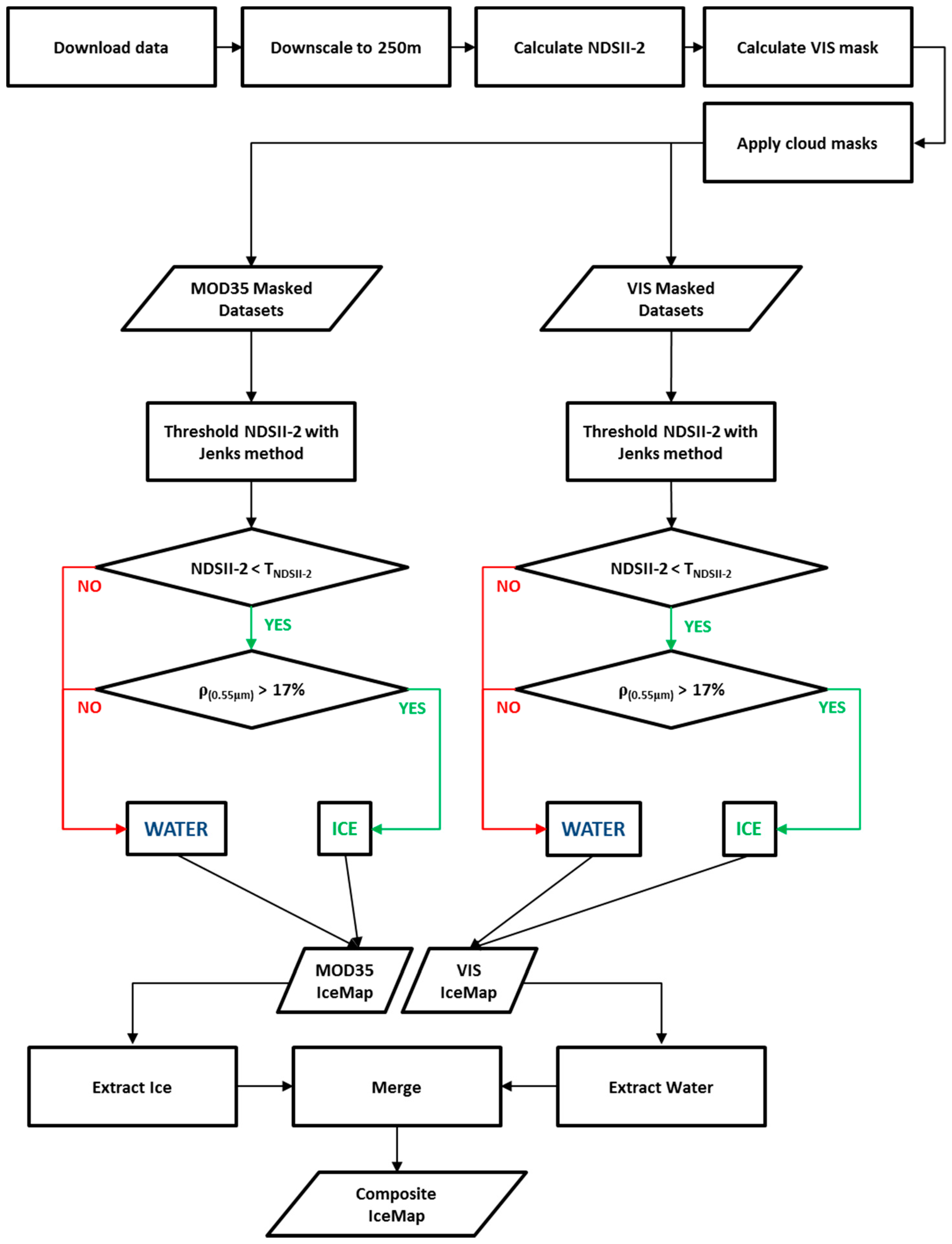
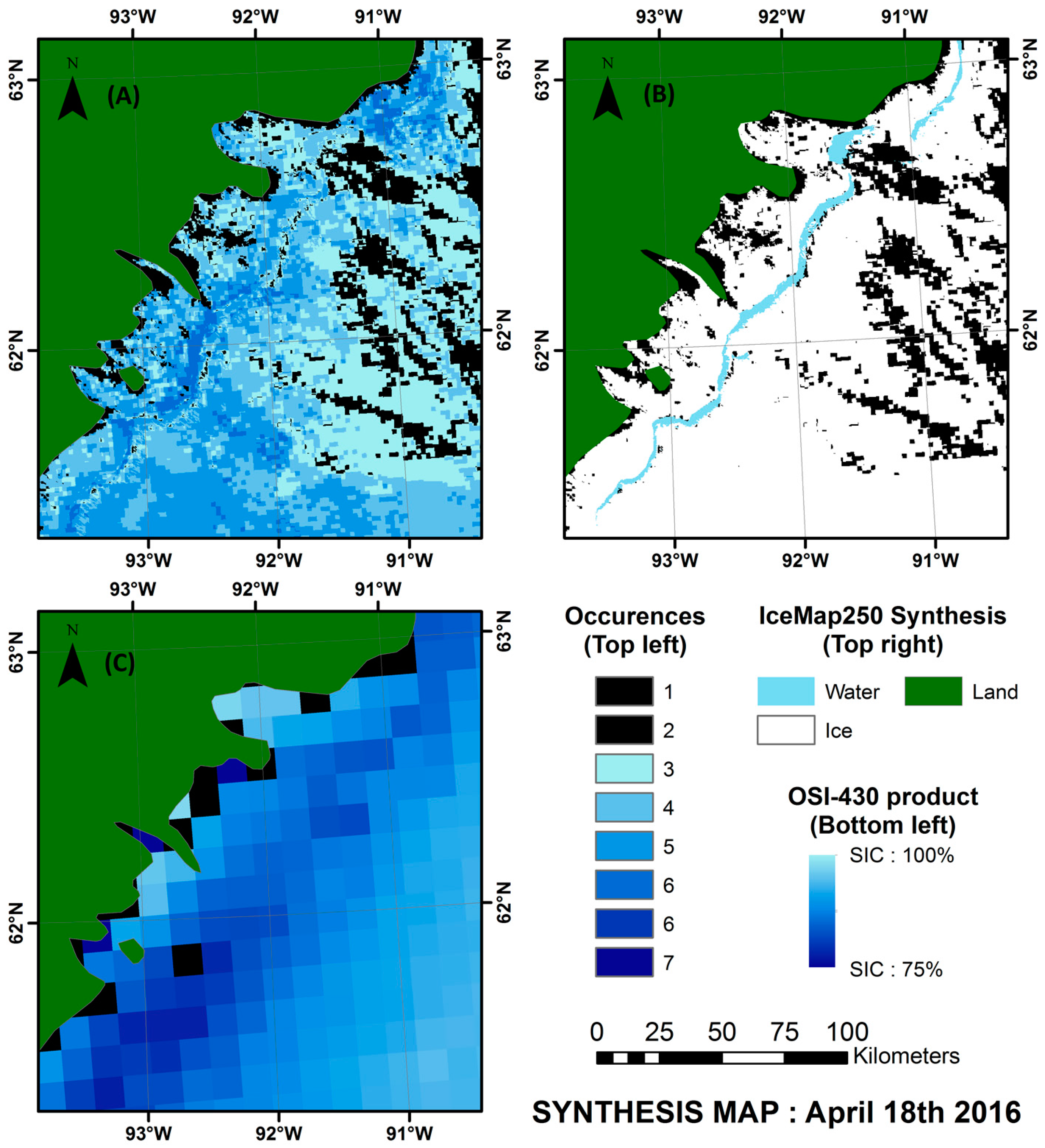
The IceMap250 algorithm automatically generates a 250 m spatial resolution ice presence map for every scene of MODIS data available over a selected territory. After processing all available scenes for a single date, for either Terra or Aqua, the algorithm builds a composite of the ice maps to obtain a unique daily ice map product.

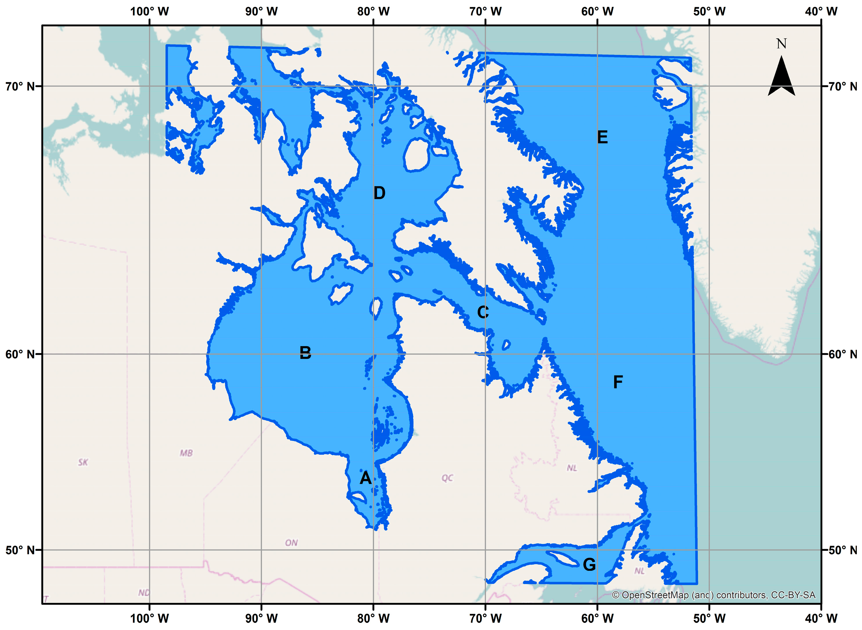
Validation of the IceMap250 products was achieved using datasets of imagery from three important periods of the sea ice regime, as described in the Section 2.2.1 of this document. Validation points, common to all evaluated products (

Table 3. IceMap250 validation components and their roles in the validation process.

Product (Mask)	Algorithm	Resolution	Role
MOD29	Original IceMap [23]	1 km	Benchmark
(MOD35)
IceMap1KM	IceMap250	1 km	Evaluate impacts of algorithm changes
(MOD35)
IceMap1KM	IceMap250	1 km	Evaluate impacts of algorithm and mask changes
(VIS)
IceMap250	IceMap250	250 m	Evaluate impacts of mask, algorithm and resolution changes
(MOD35)
IceMap250	IceMap250	250 m	Evaluate impacts of mask, algorithm and resolution changes
(VIS)
IceMap250	IceMap250	250 m	Evaluate the accuracy and performance of the final map
(Composite)

), were sampled to cumulate 500 points for each period. To gather the points for validation, a regularly spaced grid at 25 km was generated over the study domain from which points that were common to the MOD29 product and to the IceMap250 maps generated from both the MOD35 and VIS masks were kept. From these points, 500 points were randomly selected for each period for a total of 1500 validation points. Ground truth was generated manually by photo-interpretation of each point, for all three ice regime periods, based on the 250 m downscaled true color images. The validation points were selected from dates in 2013, 2015, and 2016 (see Section 2.2.1), different than those used for the calibration points used in Section 3.4.

The photo-interpretation process used is described as follows. The validation points for each scene of every ice regime period were scanned, one by one, to classify them as either ice or water. The classification for all points was performed by the same analyst for consistency. When such data was available, the classification was cross-validated using either a Landsat 7 ETM+ true color composite and/or RADARSAT-1 SAR imagery.

From these 1500 validation points, contingency tables were generated for every ice regime period to identify strengths and weaknesses of the different products. Kappa values [54] were also calculated to give a general overview of the classification performance.

4.2. Validation of the Composite Maps: Assessment of Accuracy Using Contingency Tables

The stable period contingency table (

Table 4. Contingency table for the stable period validation (10 February 2016 to 20 February 2016).

			Ground Truth
STABLE			Water	Ice	Total	Commission Error
MOD29 (M35)	Map	Water	3	6	9	66.7%
		Ice	5	486	491	1.0%
		Total	8	492	500	N/A
		Omission error	62.5%	1.2%	N/A	Overall accuracy
		Kappa	34.18%			97.80%
IceMap250 at 1 km (M35)	Map	Water	3	1	4	25.0%
		Ice	5	491	496	1.0%
		Total	8	492	500	N/A
		Omission error	62.5%	0.2%	N/A	Overall accuracy
		Kappa	49.46%			98.80%
IceMap250 at 1 km (VIS)	Map	Water	3	1	4	25.0%
		Ice	5	491	496	1.0%
		Total	8	492	500	N/A
		Omission error	62.5%	0.2%	N/A	Overall accuracy
		Kappa	49.46%			98.80%
IceMap250 (M35)	Map	Water	8	1	9	11.1%
		Ice	0	491	491	0.0%
		Total	8	492	500	N/A
		Omission error	0.0%	0.2%	N/A	Overall accuracy
		Kappa	94.02%			99.80%
IceMap250 (VIS)	Map	Water	8	1	9	11.1%
		Ice	0	491	491	0.0%
		Total	8	492	500	N/A
		Omission error	0.0%	0.2%	N/A	Overall accuracy
		Kappa	94.02%			99.80%
IceMap Composite	Map	Water	8	1	9	11.1%
		Ice	0	491	491	0.0%
		Total	8	492	500	N/A
		Omission error	0.0%	0.2%	N/A	Overall accuracy
		Kappa	94.02%			99.80%

) shows that the main error source is the mislabeling of water as sea ice. The validation results clearly show that the main factor affecting the accuracy of the maps is the spatial resolution. Considering that openings in the ice cover tend to be straight, narrow features, such as leads, during this period, the error observed in 1 km resolution products such as MOD29 could be related simply to an inability to detect these features. Since the composite map merges information from both IceMap250 MOD35 and VIS maps, it will carry the kappa score of the highest scoring, since all products are compared on common points. However, the composite map has a larger coverage than the MOD35 product since it appends the water retrieved by the VIS product.

Algorithmic changes seem to have a small, non-significant impact on accuracy. The impact of the downscaling, on the other hand, seems to be positive, as we can see from the high kappa value obtained for the IceMap250 composite map. This result has to be interpreted with parsimony, as there are only a few areas of open water that were randomly selected for the validation points (also due to their rarity during stable cover). Considering these important facts, the high kappa value of the IceMap250 MOD35, VIS, and composite should be interpreted as a sign of relative accuracy, as only one error in classifying water as ice has a significant impact on the kappa due to the small number of water pixels. When looking at Table 4, the reader should focus more on the overall accuracy than on the kappa value.

The melt period contingency table (

Table 5. Contingency table for the melt period validation (13 June 2013 to 23 June 2013).

			Ground Truth
MELT			Water	Ice	Total	Commission Error
MOD29 (M35)	Map	Water	140	5	145	3.4%
		Ice	8	347	355	2.3%
		Total	148	352	500	N/A
		Omission error	5.4%	1.4%	N/A	Overall accuracy
		Kappa	93.72%			97.40%
IceMap250 at 1 km (M35)	Map	Water	128	4	132	3.0%
		Ice	20	348	368	5.4%
		Total	148	352	500	N/A
		Omission error	13.5%	1.1%	N/A	Overall accuracy
		Kappa	88.11%			95.20%
IceMap250 at 1 km (VIS)	Map	Water	127	3	130	2.3%
		Ice	21	349	370	5.7%
		Total	148	352	500	N/A
		Omission error	14.2%	0.9%	N/A	Overall accuracy
		Kappa	88.06%			95.20%
IceMap250 (M35)	Map	Water	140	0	140	0.0%
		Ice	8	352	360	2.2%
		Total	148	352	500	N/A
		Omission error	5.4%	0.0%	N/A	Overall accuracy
		Kappa	96.10%			98.40%
IceMap250 (VIS)	Map	Water	142	0	142	0.0%
		Ice	6	352	358	1.7%
		Total	148	352	500	N/A
		Omission error	4.1%	0.0%	N/A	Overall accuracy
		Kappa	97.09%			98.80%
IceMap Composite	Map	Water	142	0	142	0.0%
		Ice	6	352	358	1.7%
		Total	148	352	500	N/A
		Omission error	4.1%	0.0%	N/A	Overall accuracy
		Kappa	97.09%			98.80%

) shows that all of the algorithms achieve high performance discriminating sea ice and water in most situations, the kappa value consistently being greater than 88%. During this period, a higher spatial resolution seems to contribute to improving the results. The melt period is characterized by its generally low extent of cloud cover when compared to freeze-up, making it easier to accurately map sea ice distribution.

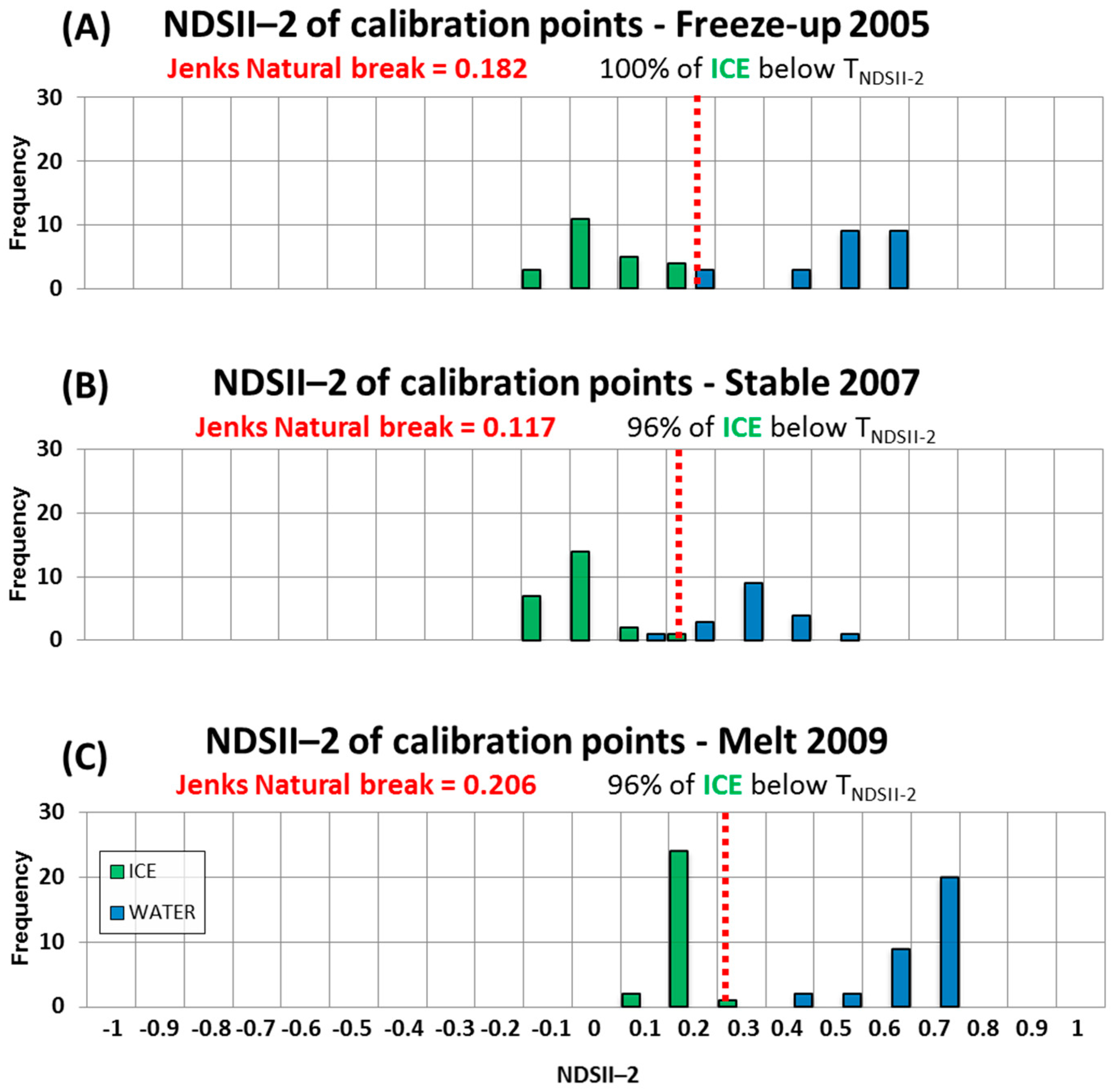
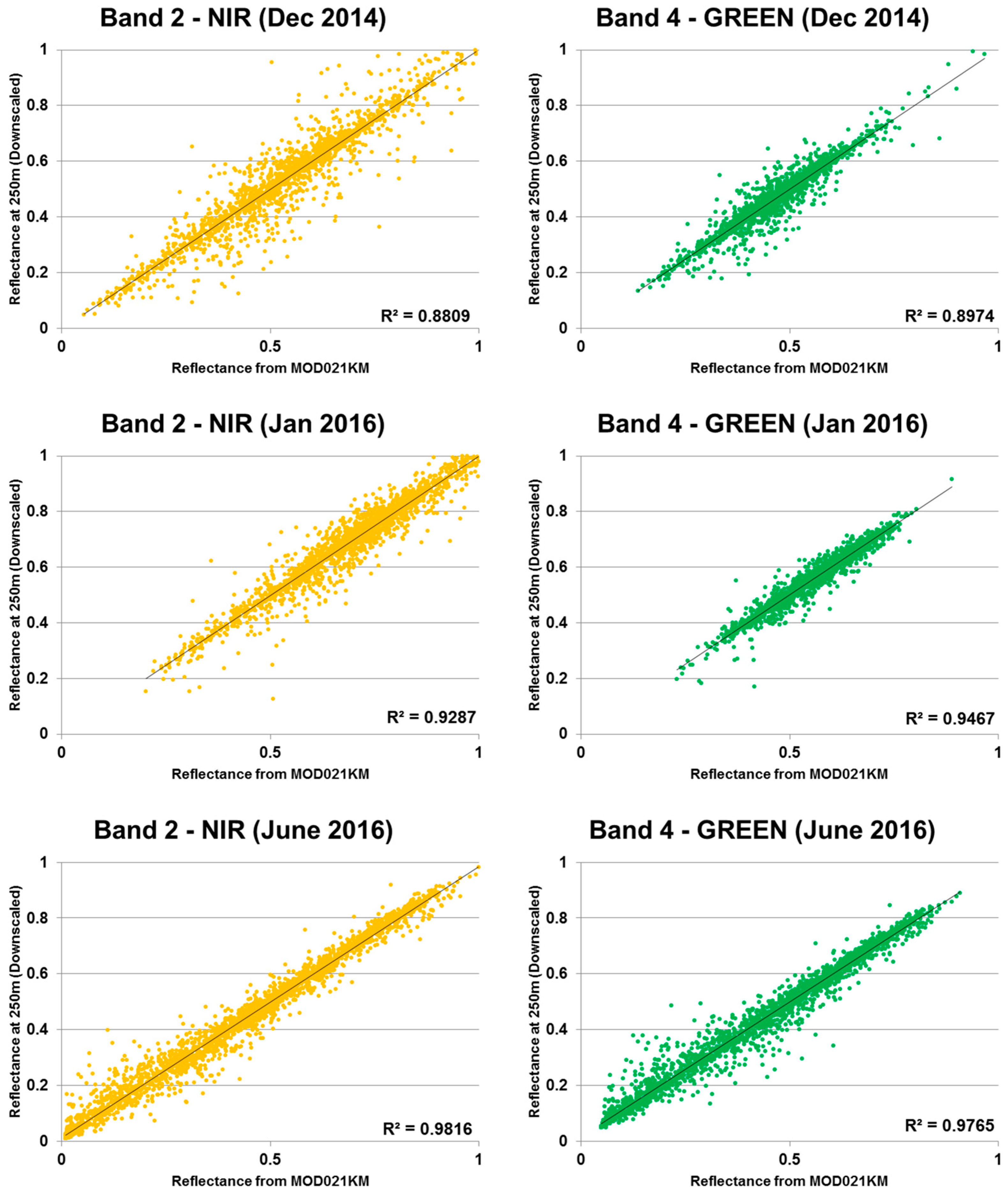
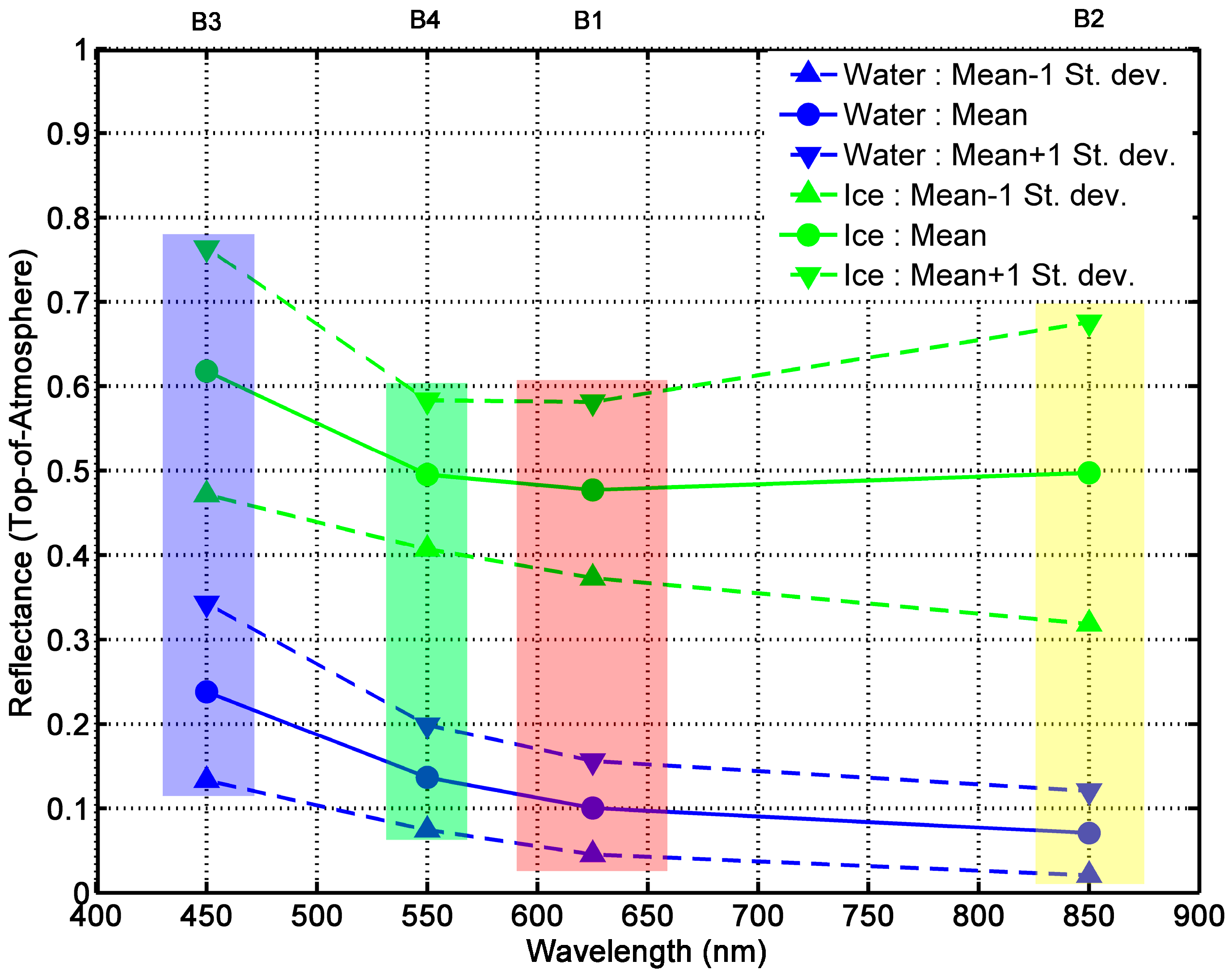
One source of error, mislabeling water as sea ice, may be linked to low tides when the intertidal area located at the outlets of rivers is exposed to the MODIS sensors. These areas are mistaken for ice as their reflectance is high at the 0.55 μm wavelength. They are adequately mapped by the original IceMap algorithm, explaining in part why the kappa score of the MOD29 product is higher than the 1 km IceMap250 products. One explanation for the improvement of the IceMap250 product at 250 m compared to its counterparts at 1 km is that the refinement brought by the downscaling makes the algorithm correct the errors in the intertidal areas since the measured T_NDSII-2 threshold is computed using different reflectances at a finer grid resolution (16 pixels at 250 m are contained in 1 pixel at 1 km), increasing the impact of these pixels in the estimation of T_NDSII-2 with the Jenks method. This situation is common in James Bay, the southernmost entity of the Hudson Bay Complex, where numerous rivers are known to bring large quantities of sediments.

Another source is the mislabeling of ice as water due to melt ponds, which, in most advanced cases, present a water-like NDSII—2 value. The 0.17 threshold used in Band 4 was shown to accurately discriminate sea ice with melt ponds from water, as about 15% of the validation points were gathered from areas with melt ponds. The slight improvement in the detection of water for the IceMap250 VIS map, compared to the 250 m MOD35 map can be explained by the difference in the extent masked by the MOD35 and the VIS masks and by the context of the melt period where water becomes more abundant. The impact on the algorithm is that the T_NDSII-2 value differs for both products because the VIS mask covers more potential water areas (high NDSII—2 values) with the effect of pulling down T_NDSII-2, resulting in more pixels failing the first test for ice detection.

The freeze-up period contingency table (

Table 6. Contingency table for the freeze-up period validation (1 December 2015 to 11 December 2015).

			Ground Truth
FREEZE-UP			Water	Ice	Total	Commission Error
MOD29 (M35)	Map	Water	78	23	101	22.8%
		Ice	3	396	399	0.8%
		Total	81	419	500	N/A
		Omission error	3.7%	5.5%	N/A	Overall accuracy
		Kappa	82.58%			94.80%
IceMap250 at 1 km (M35)	Map	Water	73	2	75	2.7%
		Ice	8	417	425	1.9%
		Total	81	419	500	N/A
		Omission error	9.9%	0.5%	N/A	Overall accuracy
		Kappa	92.41%			98.00%
IceMap250 at 1 km (VIS)	Map	Water	73	2	75	2.7%
		Ice	8	417	425	1.9%
		Total	81	419	500	N/A
		Omission error	9.9%	0.5%	N/A	Overall accuracy
		Kappa	92.41%			98.00%
IceMap250 (M35)	Map	Water	75	2	77	2.6%
		Ice	6	417	423	1.4%
		Total	81	419	500	N/A
		Omission error	7.4%	0.5%	N/A	Overall accuracy
		Kappa	93.99%			98.40%
IceMap250 (VIS)	Map	Water	74	2	76	2.6%
		Ice	7	417	424	1.7%
		Total	81	419	500	N/A
		Omission error	8.6%	0.5%	N/A	Overall accuracy
		Kappa	93.20%			98.20%
IceMap Composite	Map	Water	75	2	77	2.6%
		Ice	6	417	423	1.4%
		Total	81	419	500	N/A
		Omission error	7.4%	0.5%	N/A	Overall accuracy
		Kappa	93.99%			98.40%

) shows that the main source of error during freeze-up is the mislabeling of water as sea ice, except for the MOD29 product. The freeze-up period is especially difficult to map, mostly because of the dense cloud cover that is frequently present. The changes in the algorithm have shown, in this period, to improve the kappa value by about 10%, according to the freeze-up period validation dataset.

In some cases, a cloud-covered area will be misclassified by the cloud-masking algorithm (MOD35) and will be considered cloud-free, leading to possible mislabeling of water as ice by the IceMap250 algorithm. The low clouds and water vapor that pass through the different filters of MOD35 have negative NDSII—2 values, sufficient to pass the T_NDSII-2 threshold, and present with a high green reflectance classifying them as ice. At those same points, the NDSI values are slightly below 0.4, explaining why they do not appear as errors in the MOD29 product. Once again, the intertidal areas cause classification errors until we reach the period where the land fast ice is well established, meaning the shores display a stable ice cover.

Even though the validation data show excellent concordance with manually photo-interpreted data, it should not be taken for granted that IceMap250 will achieve such accuracy for every scene it classifies.

The validation is relative to the accuracy and consistency of the photo-interpretation, and the results could vary simply by using different validation dates. Nonetheless, given the results obtained from our extensive validation dataset, we contend that the IceMap250 classification process is reliable and generates high-quality results.

4.3. Validation of the Weekly Synthesis Maps: Comparison with Similar Products

One issue with the IceMap250 composite maps is the sparse and irregular distribution of coverage. To cope with this problem, weekly synthesis maps are generated for each of the 52 weeks of the year.

Quantitative validation is quite difficult for these synthesis maps since they are built from a collection of time-shifted datasets, but it is possible to compare them with existing synthesis products that provide a similar overview of ice presence, such as passive microwave (7 days average) and weekly maps from national ice services.

The latter products do not have the same spatial resolution as the IceMap250 synthesis map, but the comparison between these products and the IceMap250 product demonstrates the accuracy of the synthesis process used in the weekly IceMap250 maps. It is also a simple method to assess the consistency of the IceMap250 maps over time.

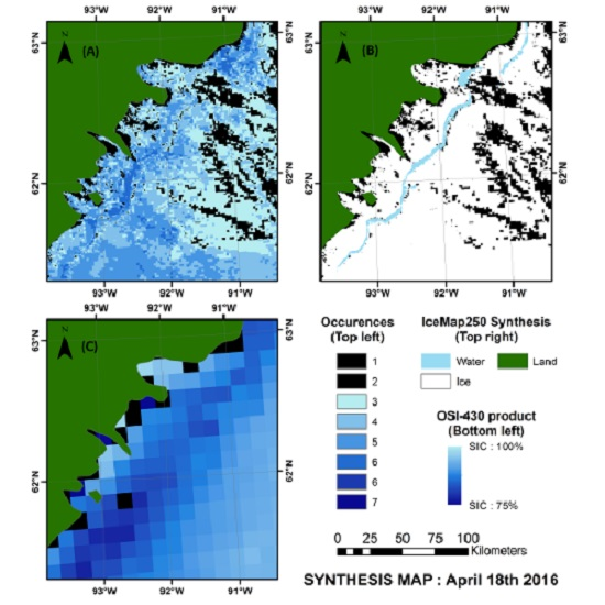
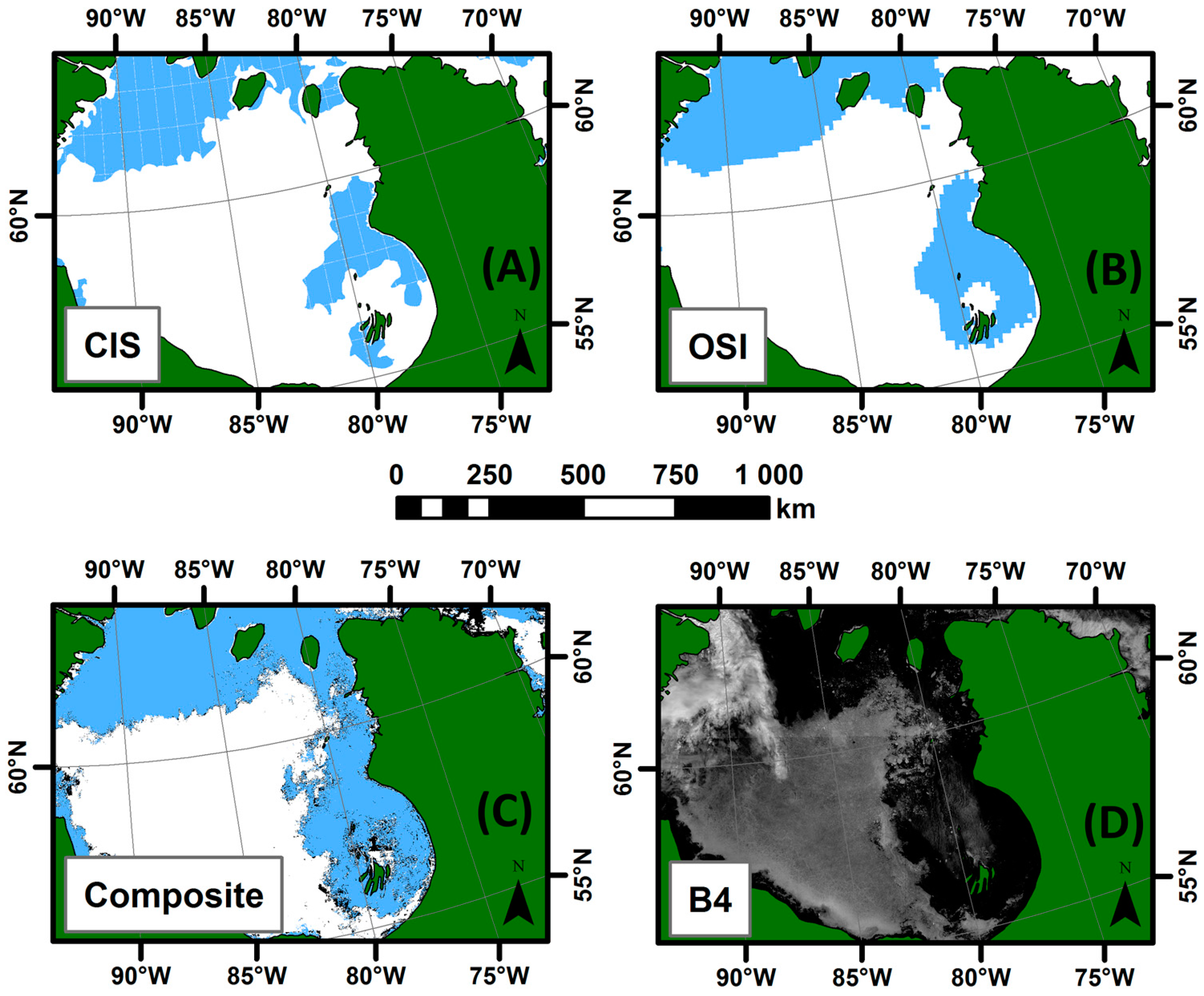
To evaluate their accuracy, the synthesis maps were then compared to the Canadian Ice Service weekly Hudson Bay regional ice charts, which are based on ScanSAR RADARSAT-1 imagery (50 or 100 m resolution), and to a 7 days average version of the OSI-409 or OSI-430 Reprocessed Sea Ice Product [55], which is based on passive microwave data with a footprint size between 30 and 50 km, sampled at every 25 km and for which the product is provided at a 12.5 km resolution. Note that the ice charts compared are potentially based on data from different days since their respective production processes and input data are different. The periods compared include the last scene within the 7 days period. A total of nine comparisons were made—one per ice season (freeze-up, stable cover and melt) for three different years. The comparison of the output weekly maps from the analysis made at the Canadian Ice Service, the passive microwave-based OSI-409 or OSI-430 (depending on the date) product and the output weekly synthesis maps from the IceMap250 algorithm (Figure 10) allow us to draw the following conclusions:

• For all three seasons considered, the general pattern and the sea ice cover agrees between the products compared.
• The IceMap250 product, contrary to the CIS maps of the OSI maps, based respectively on SAR and passive microwave data, does not map the entire area because of its vulnerability to the cloud cover.

5. Discussion

The combination of the NDSII—2 and Band 4 thresholds at 250 m showed a good performance for all three seasons of the ice regime with kappa values over 90%. The use of a Jenks natural breaks threshold on NDSII—2 values made the algorithm more flexible regarding the different ice conditions the sensor could observe at the surface, as it, by definition, adapts to the different TOA reflectance values in the domain.

One of the surfaces expected to be more difficult to adequately outline were the regions for which the ice was covered with melt ponds. According to Perovich et al. [56], the flat topography characteristic to first-year ice can bring the pond cover fraction up to 90%, which has a major impact on the pixel reflectance values. This melt pond fraction is higher than what is observed in the higher Arctic, where the melt ponds can cover up to 50%–60% of sea ice during the boreal summer [57,58].

When mapping ice with melt ponds, which according to Rosel et al. [59] can appear as soon as mid-April in the Southern Arctic, as confirmed by our imagery, the NDSII-2 information showed to be insufficient when used alone for cases of an advanced melt state. However, thresholding on Band 4 (TOA reflectance >0.17 in green) showed to effectively discriminate ice with melt ponds from water, as the mislabeling of sea ice as water is lower for all IceMap250 products than for the MOD29 product, regardless of the resolution. This discrimination capacity in the green band is coherent according to the spectral signature curves of water and melt ponds (deep blue ponds, blue-green ponds, dark ponds) [60]. One interesting development avenue for the algorithm would be to test the NDSII-2 values to see if the detection of melt ponds is possible.

The refinement in spatial resolution gives the algorithm the capacity to detect smaller features that would not be visible at a 1 km resolution. The downscaled images, compared on a point-by-point basis, show that the CCRS algorithm [26,43] performs very well at downscaling MODIS images to 250 m, even when conditions are not optimal due to cloud cover like in the freeze-up period (Figure 11), and that it is an appropriate tool for studying sea ice cover as it does not alter or distort the spectral properties of the scene [58]. Correlation between Bands 2 and 4 at 1 km grid resolution and their 250 m downscaled counterparts showed that, for all three seasons and on more than 1500 points per period, the lowest R² value has shown to be 0.88. Even if the downscaling algorithm performs well, classification errors can certainly be linked to this process, especially for sectors of the image where the pixel TOA reflectance values are close to the threshold values. This downscaling plays an important role in the overall quality of the IceMap250 composite map.

Cloud cover is the most restrictive barrier to sea ice mapping using optical data. This is particularly true during the freeze-up season when all the algorithms tested display their lowest overall accuracy. As an example, for the three periods of the ice regime in 2003, under the hybrid mask (MOD35 + VIS), the maximum occurrence percentage of cloud-free pixels was 57% for the stable cover period, 66% for the melt period, and 42% for the freeze-up period. A recurrent pattern of cloud cover, intimately linked with the formation of sea ice, was observed that year in the Hudson Bay. Ice first developed and last melted in the southwestern part of the bay, where visibility seemed to be at its maximum in all periods of the ice regime.

The best performance for the IceMap250 performance is not seen when the VIS mask is used alone, which could trigger false positives of sea ice presence, but when it is used in combination with the MOD35 mask to achieve the composite map. As well, classification errors are certainly linked to the use of a suboptimal land mask, with a resolution coarser than the satellite imagery used in the algorithm. The use of a better mask would reduce land contamination errors. The overall performance of the IceMap250 algorithm is intimately linked to the land and cloud masking quality.

6. Conclusions

The fully automated IceMap250 algorithm provides 250 m of sea ice presence maps using the highest possible resolution data from the MODIS-Terra or Aqua sensors and specialized downscaling techniques, an improvement when compared to the original approach. Additionally, IceMap250 uses a different spectral ratio to detect sea ice. Using the NIR band instead of the SWIR band, the NDSII—2 index provides excellent results and makes the algorithm fully compatible with both MODIS platforms.

As expected, the impact of cloud cover on the spatial extent covered by the maps is major, especially during the freeze-up season, when the waters of Hudson Bay are warmer than the Arctic air masses, generating massive cloud formation. Nevertheless, when under clear sky conditions and adequately masked, the approach is efficient and accurate. Further improvement of the cloud-masking algorithms for the MODIS platform will necessarily have a positive impact on false sea ice detection in the IceMap250 algorithm.

Both quantitative and visual comparisons confirm that the IceMap250 maps are a useful source of ice information, even on a weekly scale. The general spatial pattern of the sea ice cover is respected in every case, and the approach offers the advantage of quickly providing fine ice cover details as soon as the MODIS imagery is available (near real time production).

The IceMap250 algorithm generates reliable and accurate sea ice detection data, in all cases with a kappa value over 90%, which would constitute an excellent backbone to any ice presence study; the algorithm thus has the potential to be used for numerous scientific and operational applications.

References

1. Public Infrastructure Engineering Vulnerability Committee (PIEVC). Adapting to Climate Change—Canada's First National Assessment of Public Infrastructure; Council of Professional Engineers: Ottawa, ON, Canada, 2008. [Google Scholar]
2. Ivanova, N.; Pedersen, L.; Tonboe, R.; Kern, S.; Heygster, G.; Lavergne, T.; Sorensen, A.; Saldo, R.; Dybkjar, G.; Brucker, L. Inter-comparison and evaluation of sea ice algorithms: Towards further identification of challenges and optimal approach using passive microwave observations. Cryosphere 2015, 9, 1797–1817. [Google Scholar] [CrossRef] [Green Version]
3. Markus, T.; Cavalieri, D.J. An enhancement of the nasa team sea ice algorithm. IEEE Trans. Geosci. Remote Sens. 2000, 38, 1387–1398. [Google Scholar] [CrossRef]
4. Shokr, M.; Lambe, A.; Agnew, T. A new algorithm (ECICE) to estimate ice concentration from remote sensing observations: An application to 85-GHZ passive microwave data. IEEE Trans. Geosci. Remote Sens. 2008, 46, 4104–4121. [Google Scholar] [CrossRef]
5. Spreen, G.; Kaleschke, L.; Heygster, G. Sea ice remote sensing using amsr-e 89-GHz channels. J. Geophys. Res. Oceans 2008. [Google Scholar] [CrossRef]
6. Scheuchl, B.; Caves, R.; Cumming, I.; Staples, G. Automated sea ice classification using spaceborne polarimetric sar data. In Proceedings of the 2001 IEEE International Geoscience and Remote Sensing Symposium, Sydney, Ausralia, 9–13 July 2001.
7. Soh, L.-K.; Tsatsoulis, C.; Gineris, D.; Bertoia, C. Arktos: An intelligent system for sar sea ice image classification. IEEE Trans. Geosci. Remote Sens. 2004, 42, 229–248. [Google Scholar] [CrossRef]
8. Yu, Q.; Clausi, D.A. Sar sea-ice image analysis based on iterative region growing using semantics. IEEE Trans. Geosci. Remote Sens. 2007, 45, 3919–3931. [Google Scholar] [CrossRef]
9. Drue, C.; Heinemann, G. High-resolution maps of the sea-ice concentration from modis satellite data. Geophys. Res. Lett. 2004, 31, 08027. [Google Scholar] [CrossRef]
10. Hall, D.K.; Key, J.R.; Casey, K.A.; Riggs, G.A.; Cavalieri, D.J. Sea ice surface temperature product from MODIS. IEEE Trans. Geosci. Remote Sens. 2004, 42, 1076–1087. [Google Scholar] [CrossRef]
11. Hori, M.; Aoki, T.; Stamnes, K.; Li, W. Adeos-II/GLI snow/ice products—Part III: Retrieved results. Remote Sens. Environ. 2007, 111, 291–336. [Google Scholar] [CrossRef]
12. Shokr, M.; Sinha, N. Sea Ice: Physics and Remote Sensing; John Wiley & Sons: Hoboken, NJ, USA, 2015. [Google Scholar]
13. Crocker, G.B.; Carrieres, T. The Canandian Ice Service Digital Datedbse: History of Data and Procedures Used in the Preparation of Regional Ice Charts; Ballicater Consulting Ltd.: Ottawa, ON, Canada, 2000. [Google Scholar]
14. Kaleschke, L.; Lupkes, C.; Vihma, T.; Haarpaintner, J.; Bochert, A.; Hartmann, J.; Heygster, G. SSM/I sea ice remote sensing for mesoscale ocean-atmosphere interaction analysis. Can. J. Remote Sens. 2001, 27, 526–537. [Google Scholar] [CrossRef]
15. Kern, S. A new method for medium-resolution sea ice analysis using weather-influence corrected special sensor microwave/imager 85 GHz data. Int. J. Remote Sens. 2004, 25, 4555–4582. [Google Scholar] [CrossRef]
16. Beitsch, A.; Kaleschke, L.; Kern, S. Investigating high-resolution AMSR2 sea ice concentrations during the February 2013 fracture event in the beaufort sea. Remote Sens. 2014, 6, 3841–3856. [Google Scholar] [CrossRef]
17. Agnew, T.; Howell, S. The use of operational ice charts for evaluating passive microwave ice concentration data. Atmos. Ocean 2003, 41, 317–331. [Google Scholar] [CrossRef]
18. Rees, W.G. Remote Sensing of Snow and Ice; CRC Press: Boca Raton, FL, USA, 2005. [Google Scholar]
19. Meier, W.N.; Fetterer, F.; Stewart, J.S.; Helfrich, S. How do sea-ice concentrations from operational data compare with passive microwave estimates? Implications for improved model evaluations and forecasting. Ann. Glaciol. 2015, 56, 332–340. [Google Scholar] [CrossRef]
20. Meier, W.N.; Stroeve, J. Comparison of sea-ice extent and ice-edge location estimates from passive microwave and enhanced-resolution scatterometer data. Ann. Glaciol. 2008, 48, 65–70. [Google Scholar] [CrossRef]
21. Heinrichs, J.F.; Cavalieri, D.J.; Markus, T. Assessment of the Amsr-E sea ice-concentration product at the ice edge using radarsat-1 and modis imagery. IEEE Trans. Geosci. Remote Sens. 2006, 44, 3070–3080. [Google Scholar] [CrossRef]
22. Meier, W.N. Comparison of passive microwave ice concentration algorithm retrievals with avhrr imagery in Arctic peripheral seas. IEEE Trans. Geosci. Remote Sens. 2005, 43, 1324–1337. [Google Scholar] [CrossRef]
23. Hall, D.K.; Riggs, G.A.; Salomonson, V.V.; Barton, J.; Casey, K.; Chien, J.; DiGirolamo, N.; Klein, A.; Powell, H.; Tait, A. Algorithm Theoretical Basis Document (ATBD) for the MODIS Snow and Sea Ice-Mapping Algorithms; NASA GSFC: Greenbelt, MD, USA, 2001. [Google Scholar]
24. Su, H.; Wang, Y.; Xiao, J.; Li, L. Improving modis sea ice detectability using gray level co-occurrence matrix texture analysis method: A case study in the bohai sea. ISPRS J. Photogramm. Remote Sens. 2013, 85, 13–20. [Google Scholar] [CrossRef]
25. Su, H.; Wang, Y.; Yang, J. Monitoring the spatiotemporal evolution of sea ice in the bohai sea in the 2009–2010 winter combining MODIS and meteorological data. Estuar. Coasts 2012, 35, 281–291. [Google Scholar] [CrossRef]
26. Liu, Y.; Key, J.; Mahoney, R. Sea and freshwater ice concentration from viirs on suomi npp and the future jpss satellites. Remote Sens. 2016, 8, 523. [Google Scholar] [CrossRef]
27. Luo, Y.; Trishchenko, A.P.; Khlopenkov, K.V. Developing clear-sky, cloud and cloud shadow mask for producing clear-sky composites at 250-meter spatial resolution for the seven MODIS land bands over canada and North America. Remote Sens. Environ. 2008, 112, 4167–4185. [Google Scholar] [CrossRef]
28. Keshri, A.K.; Shukla, A.; Gupta, R.P. Aster ratio indices for supraglacial terrain mapping. Int. J. Remote Sens. 2008, 30, 519–524. [Google Scholar] [CrossRef]
29. Canadian-Ice-Service. Sea Ice Climatic Atlas for the Northern Canadian Waters 1981–2010. Available online: https://ec.gc.ca/glaces-ice/default.asp?lang=En&n=4B35305B-1 (accessed on 24 October 2016).
30. Riggs, G.A.; Hall, D.K. Snow mapping with the MODIS aqua instrument. In Proceedings of the 61st Eastern Snow Conference, Portland, OR, USA, 9–11 June 2004; pp. 9–11.
31. Natural Earth. Coastline. Available online: http://www.naturalearthdata.com/downloads/110m-physical-vectors/110m-coastline/ (accessed on 24 October 2016).
32. Wessel, P.; Smith, W.H.F. A global, self-consistent, hierarchical, high-resolution shoreline database. J. Geophys. Res. Solid Earth 1996, 101, 8741–8743. [Google Scholar] [CrossRef]
33. Perovich, D.K.; Polashenski, C. Albedo evolution of seasonal Arctic sea ice. Geophys. Res. Lett. 2012. [Google Scholar] [CrossRef]
34. Perovich, D.K. Light reflection from sea ice during the onset of melt. J. Geophys. Res. Oceans 1994, 99, 3351–3359. [Google Scholar] [CrossRef]
35. Perovich, D.K. The Optical Properties of Sea Ice; DTIC: Fort Belvoir, VA, USA, 1996. [Google Scholar]
36. Barber, D.G.; Misurak, K.; Ledrew, E. Spectral albedo of snow-covered first-year and multi-year sea ice during spring melt. Ann. Glaciol. 1995, 21, 337–342. [Google Scholar]
37. Fan, C.; Warner, R.A. Characterization of water reflectance spectra variability: Implications for hyperspectral remote sensing in estuarine waters. Mar. Sci. 2014, 4, 1–9. [Google Scholar]
38. Clark, R.N.; Swayze, G.A.; Wise, R.; Livo, K.E.; Hoefen, T.M.; Kokaly, R.F.; Sutley, S.J. USGS Digital Spectral Library Splib06a; US Geological Survey: Reston, VA, USA, 2007. [Google Scholar]
39. Baldridge, A.; Hook, S.; Grove, C.; Rivera, G. The ASTER spectral library version 2.0. Remote Sens. Environ. 2009, 113, 711–715. [Google Scholar] [CrossRef]
40. Perovich, D.K. Observations of the polarization of light reflected from sea ice. J. Geophys. Res. Oceans 1998, 103, 5563–5575. [Google Scholar] [CrossRef]
41. Dozier, J. Spectral signature of alpine snow cover from the landsat thematic mapper. Remote Sens. Environ. 1989, 28, 9–22. [Google Scholar] [CrossRef]
42. Bishop, M.P.; Bjornsson, H.; Haeberli, W.; Oerlemans, J.; Shroder, J.F.; Tranter, M.; Singh, V.P.; Haritashya, U.K. Encyclopedia of Snow, Ice and Glaciers; Springer: Berlin, Germany, 2011. [Google Scholar]
43. Riggs, G.A.; Hall, D.K.; Ackerman, S.A. Sea ice extent and classification mapping with the moderate resolution imaging spectroradiometer airborne simulator. Remote Sens. Environ. 1999, 68, 152–163. [Google Scholar] [CrossRef]
44. Trishchenko, A.P.; Luo, Y.; Khlopenkov, K.V. A method for downscaling MODIS land channels to 250-m spatial resolution using adaptive regression and normalization. Proc. SPIE 2006. [Google Scholar] [CrossRef]
45. Xiao, X.; Shen, Z.; Qin, X. Assessing the potential of vegetation sensor data for mapping snow and ice cover: A normalized difference snow and ice index. Int. J. Remote Sens. 2001, 22, 2479–2487. [Google Scholar] [CrossRef]
46. El-Alem, A.; Chokmani, K.; Laurion, I.; El-Adlouni, S. An adaptive model to monitor chlorophyll-a in inland waters in southern quebec using downscaled MODIS imagery. Remote Sens. 2014, 6, 6446–6471. [Google Scholar] [CrossRef]
47. Fontana, F.M.A.; Trishchenko, A.P.; Luo, Y.; Khlopenkov, K.V.; Nussbaumer, S.U.; Wunderle, S. Perennial snow and ice variations (2000–2008) in the Arctic circumpolar land area from satellite observations. J. Geophys. Res. Earth Surf. 2010. [Google Scholar] [CrossRef]
48. Gu, Y.; Wylie, B. Downscaling 250-m modis growing season ndvi based on multiple-date landsat images and data mining approaches. Remote Sens. 2015, 7, 3489–3506. [Google Scholar] [CrossRef]
49. Trishchenko, A.P.; Khlopenkov, K.V.; Ungureanu, C.; Latifovic, R.; Luo, Y.; Park, W.B. Mapping of surface albedo over mackenzie river basin from satellite observations. In Cold Region Atmospheric and Hydrologic Studies. The Mackenzie Gewex Experience; Springer: Berlin, Germany, 2008; pp. 327–341. [Google Scholar]
50. Ackerman, S.A.; Strabala, K.I.; Menzel, W.P.; Frey, R.A.; Moeller, C.C.; Gumley, L.E. Discriminating clear sky from clouds with MODIS. J. Geophys. Res. Atmos. 1998, 103, 32141–32157. [Google Scholar] [CrossRef]
51. Kilpatrick, K.A.; Podesta, G.; Walsh, S.; Williams, E.; Halliwell, V.; Szczodrak, M.; Brown, O.B.; Minnett, P.J.; Evans, R. A decade of sea surface temperature from modis. Remote Sens. Environ. 2015, 165, 27–41. [Google Scholar] [CrossRef]
52. Chan, M.A.; Comiso, J.C. Arctic cloud characteristics as derived from modis, calipso, and cloudsat. J. Clim. 2013, 26, 3285–3306. [Google Scholar] [CrossRef]
53. Jenks, G.F. The data model concept in statistical mapping. Int. Yearb. Cartogr. 1967, 7, 186–190. [Google Scholar]
54. Congalton, R.G. A review of assessing the accuracy of classifications of remotely sensed data. Remote Sens. Environ. 1991, 37, 35–46. [Google Scholar] [CrossRef]
55. Eastwood, S.; Jenssen, M.; Lavergne, T.; Sorensen, A.; Tonboe, R. Global Sea Ice Concentration Reprocessing—Product User Manual; Ocean and Sea Ice SAF-Eumetsat: Darmstadt, Germany, 2015. [Google Scholar]
56. Perovich, D.; Jones, K.; Light, B.; Eicken, H.; Markus, T.; Stroeve, J.; Lindsay, R. Solar partitioning in a changing Arctic sea-ice cover. Ann. Glaciol. 2011, 52, 192–196. [Google Scholar] [CrossRef]
57. Eicken, H.; Grenfell, T.C.; Perovich, D.K.; Richter-Menge, J.A.; Frey, K. Hydraulic controls of summer Arctic pack ice albedo. J. Geophys. Res. Oceans 2004. [Google Scholar] [CrossRef]
58. Fetterer, F.; Untersteiner, N. Observations of melt ponds on Arctic sea ice. J. Geophys. Res. Oceans 1998, 103, 24821–24835. [Google Scholar] [CrossRef]
59. Rosel, A.; Kaleschke, L.; Birnbaum, G. Melt ponds on Arctic sea ice determined from MODIS satellite data using an artificial neural network. Cryosphere 2012, 6, 431–446. [Google Scholar] [CrossRef] [Green Version]
60. Tschudi, M.A.; Maslanik, J.A.; Perovich, D.K. Derivation of melt pond coverage on Arctic sea ice using modis observations. Remote Sens. Environ. 2008, 112, 2605–2614. [Google Scholar] [CrossRef]
Figure 1. Test area for IceMap250, including James Bay (A), Hudson Bay (B), Hudson Strait (C), Foxe Basin (D), Davis Strait (E), Labrador coast (F), and part of the Gulf of Saint-Lawrence (G), all located in eastern Canada.
Remotesensing 09 00070 g001
Figure 2. Reference spectrums for different types of ice cover at different states based on USGS [38] and ASTER [39] spectral libraries and from field observations by Perovich in 1998 [40]. These spectrums are solely presented to display the variations in reflectances of the different surfaces encountered by IceMap250.
Remotesensing 09 00070 g002
Figure 3. Processing flowchart of the IceMap250 algorithm. In this figure, ρ(0.55 μm) represents the TOA reflectance in the green band, and TNDSII-2 is the threshold of NDSII-2 obtained using the Jenks natural breaks method.
Remotesensing 09 00070 g003
Figure 4. (AD) Comparison of the 3 snow detection indices on a MODIS Terra scene for 12 June 2015. The scene is characterized by a low cloud cover, the presence of melted snow along the eastern coast, the presence of a clear open water area and of a mixed region of open water and small ice floes in the northwest. B1 to B6 denote the MODIS Bands 1 to 6. Areas shown in black are areas where no sea ice information was available due to the cloud cover.
Remotesensing 09 00070 g004
Figure 5. (A,B) Downscaling example over Ungava Bay in the Hudson Strait area on 15 March 2014. The original 500 m Band 4 (green band) data is on the left and the downscaled result at 250 m is on the right.
Remotesensing 09 00070 g005
Figure 6. Water (W) and Ice (I) sample TOA reflectance values for Bands 1 to 4 and for all periods of the ice regime combined.
Remotesensing 09 00070 g006
Figure 7. (AC) Distribution of photo-interpreted calibration data points compared to the obtained TNDSII-2 threshold values obtained using Jenks Natural break method for all periods of the ice regime.
Remotesensing 09 00070 g007
Figure 8. (AD) An example of the composition process for 4 July 2009. The composite IceMap250 is the fusion of the water detected in IceMap250 with VIS and the ice detected in IceMap250 with MOD35. Cloudy pixels or pixels where the classification failed to provide a consistent result appear in black in the IceMap250 maps. (The IceMap250 maps are to be made available to users through the IcePAC web interface at http://icepac.ete.inrs.ca).
Remotesensing 09 00070 g008
Figure 9. (AC) Information occurrence map, IceMap250 7-days synthesis map (250 m), and OSI-430 (12.5 km) sea ice concentrations (SIC) for 18 April 2016. For the occurrence map, black pixels are pixels with less than 3 occurrences of data in the 7 days period. For the OSI-430 map, the black pixels are areas considered as land at the passive microwave data grid resolution.
Remotesensing 09 00070 g009
Figure 10. Comparison of ice extent as depicted by the CIS weekly map (A), the OSI 7 days average (B), the IceMap250 composite map (C), and the green band of MODIS (D) for 27 June 2016. Sea ice is presented in white and water in blue. Black pixels in the composite map denote missing data.
Remotesensing 09 00070 g010
Figure 11. Agreement between the TOA reflectances of the MOD021KM Bands 2 and 4 and the downscaled bands at 250 m grid resolution generated by the CCRS algorithm for 3 different scenes during freeze-up, stable cover, and melt periods.
Remotesensing 09 00070 g011