
MODIS Time Series to Detect Anthropogenic Interventions and Degradation Processes in Tropical Pasture

 and
and
Abstract
:
1. Introduction
Theoretical Basis for Tropical Pastures Assessment Using EVI2 Time Series
2. Materials and Methods
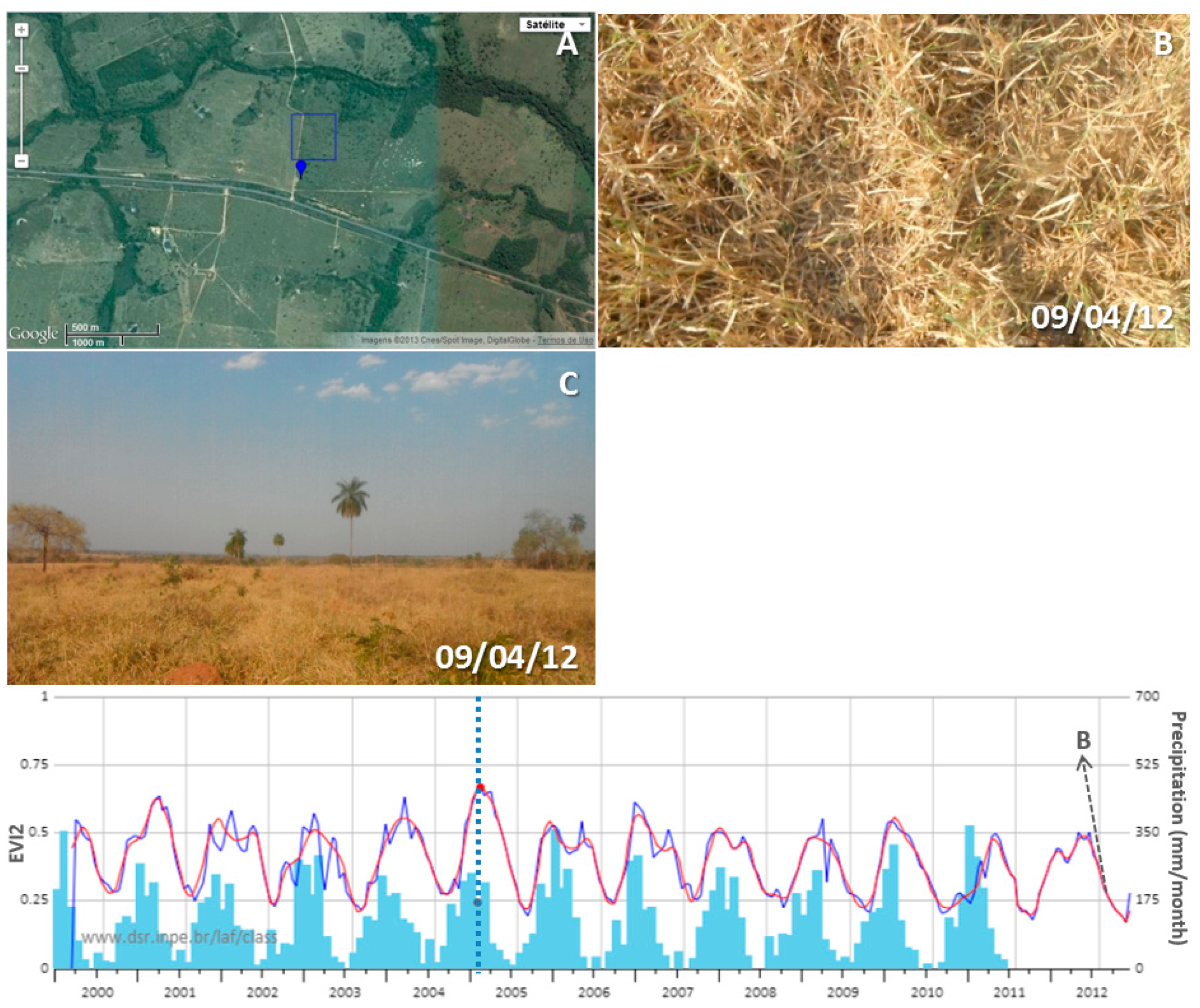
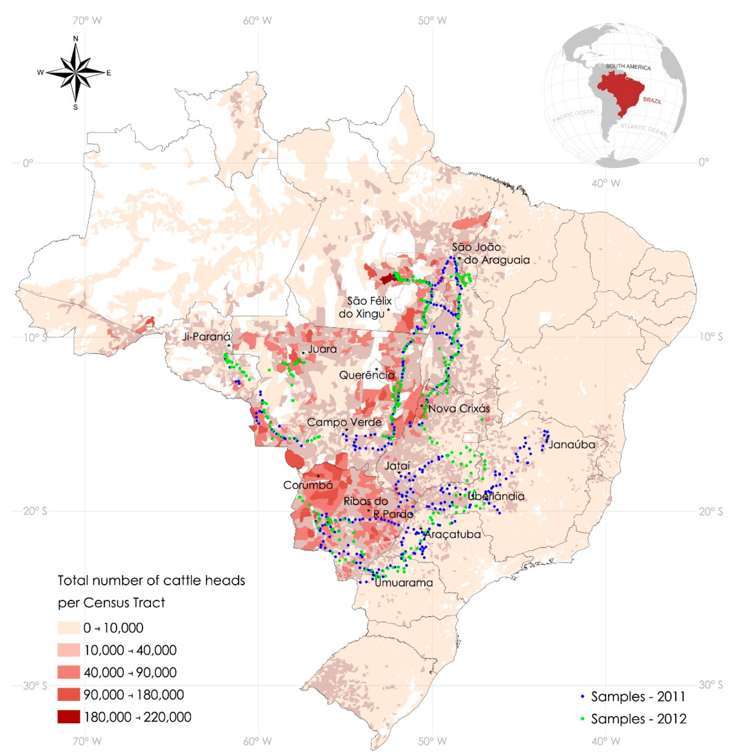
2.1. Study Area and Field Campaigns
2.2. In Situ Pasture Data Collection
2.3. Remotely Sensed Data
2.3.1. Protocol for Pasture Assessment Using Vegetation Index Time Series
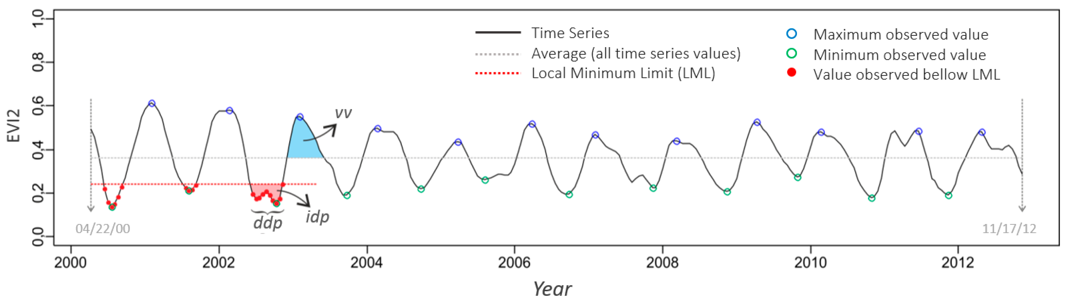
2.3.2. Phenological Metrics
Boolean Criteria and Numeric Comparisons
2.3.3. Identification of Anthropogenic Intervention in the Pasture
2.3.4. Identification of Degradation Process in Pasture
3. Results
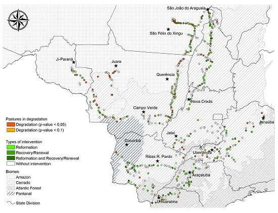
3.1. Regional Analysis
3.2. Degradation and Intensification Trends in the Sampled Pasture Lands
4. Discussion
4.1. Anthropogenic Interventions
4.2. Degradation Process
4.3. Caveats
5. Conclusions
Acknowledgments
Author Contributions
Conflicts of Interest
Appendix A
References
- Tilman, D.; Balzer, C.; Hill, J.; Befort, B.L. Global food demand and the sustainable intensification of agriculture. Proc. Natl. Acad. Sci. USA 2011, 108, 20260–20264. [Google Scholar] [CrossRef] [PubMed]
- Edenhofer, O.; Madruga, R.P.; Sokona, Y.; Seyboth, K.; Matschoss, P.; Kadner, S.; Zwickel, T.; Eickemeier, P.; Hansen, G.; Schlömer, S.; et al. IPCC special report on renewable energy sources and climate change mitigation. In Working Group III of the Intergovernmental Panel on Climate Change; Cambridge University Press: Cambridge, UK, 2011; p. 1075. [Google Scholar]
- Bedunah, D.J.; Angerer, J.P. Rangeland degradation, poverty, and conflict: How can rangeland scientists contribute to effective responses and solutions? Rangel. Ecol. Manag. 2012, 65, 606–612. [Google Scholar] [CrossRef]
- Herrick, J.E.; Brown, J.R.; Bestelmeyer, B.T.; Andrews, S.S.; Baldi, G.; Davies, J.; Duniway, M.; Havstad, K.M.; Karl, J.W.; Karlen, D.L.; et al. Revolutionary land use change in the 21st century: Is (rangeland) science relevant? Rangel. Ecol. Manag. 2012, 65, 590–598. [Google Scholar] [CrossRef]
- Food and Agriculture Organization (FAO). World Agriculture: Statistics, Roma, 2013. Available online: http://www.fao.org/statistics/en/ (accessed on 18 June 2013).
- COP: Panorama. Available online: http://www.brasil.gov.br/cop/panorama/o-que-o-brasil-esta-fazendo/metas-domesticas (accessed on 11 July 2013).
- Smith, P.; Bustamante, M.; Ahammad, H.; Clark, H.; Dong, H.; Elsiddig, E.A.; Haberl, H.; Harper, R.; House, J.; Jafari, M.; et al. Agriculture, forestry and other land use (AFOLU). In Climate Change 2014: Mitigation of Climate Change. Contribution of Working Group III to the Fifth Assessment Report of the Intergovernmental Panel on Climate Change; Edenhofer, O., Madruga, R.P., Sokona, Y., Farahani, E., Kadner, S., Seyboth, K., Adler, A., Baum, I., Brunner, S., Eickemeier, P., et al., Eds.; Cambridge University Press: Cambridge, UK, 2014. [Google Scholar]
- Scharlemann, P.W.; Laurance, W.F. How green are biofuels? Science 2008, 319, 43–44. [Google Scholar] [CrossRef] [PubMed]
- Goldemberg, J.; Guardabassi, P. Are biofuels a feasible option? Energy Policy 2009, 37, 10–14. [Google Scholar] [CrossRef]
- Leite, R.C.C.; Leal, M.R.L.V.; Cortez, L.A.B.; Griffin, W.M.; Scandiffio, M.I.G. Can Brazil replace 5% of the 2025 gasoline world demand with ethanol? Energy 2009, 65, 655–661. [Google Scholar] [CrossRef]
- Nair, P.K.R.; Saha, S.K.; Nair, V.D.; Haile, S.G. Potential for greenhouse gas emissions from soil carbon stock following biofuel cultivation on degraded lands. Land Degrad. Dev. 2011, 22, 395–409. [Google Scholar] [CrossRef]
- Filho, M.B.D. Degradação de Pastagens: Processos, Causas e Estratégias de Recuperação, 4th ed.; Embrapa Amazônia Oriental: Belém, Brazil, 2011; p. 215. [Google Scholar]
- Numata, I.; Roberts, D.A.; Chadwick, O.A.; Schimel, J.; Sampaio, F.R.; Leonidas, F.C. Regional characterization of pasture changes through time and space in Rondônia, Brazil. Earth Interact. 2007, 11, 1–25. [Google Scholar] [CrossRef]
- Numata, I.; Roberts, D.A.; Chadwick, O.A.; Schimel, J.; Sampaio, F.R.; Leonidas, F.C.; Soares, J.V. Characterization of pasture biophysical properties and the impact of grazing intensity using remotely sensed data. Remote Sens. Environ. 2007, 109, 314–327. [Google Scholar] [CrossRef]
- Davidson, E.A.; Asner, G.P.; Stone, T.A.; Neill, C.; Figueiredo, R.O. Objective indicators of pasture degradation from spectral mixture analysis of Landsat imagery. J. Geophys. Res. Biogeosci. 2008, 113. [Google Scholar] [CrossRef]
- Rufin, P.; Müller, H.; Pflugmacher, D.; Hostert, P. Land use intensity trajectories on Amazonian pastures derived from Landsat time series. Int. J. Appl. Earth Obs. Geoinf. 2015, 41, 1–10. [Google Scholar] [CrossRef]
- Allen, R.A.W.; West, N.E.; Ramsey, R.D.; Efroymson, R.A. A Protocol for retrospective remote sensing: Based ecological monitoring of rangelands. Rangel. Ecol. Manag. 2008, 59, 19–29. [Google Scholar] [CrossRef]
- Hagen, S.C.; Heilman, P.; Marsett, R.; Torbick, N.; Salas, W.; van Ravensway, J.; Qi, J. Mapping total vegetation cover across western rangelands with moderate-resolution imaging spectroradiometer data. Rangel. Ecol. Manag. 2012, 65, 456–467. [Google Scholar] [CrossRef]
- Wylie, B.K.; Boyte, S.P.; Major, D.J. Ecosystem performance monitoring of rangelands by integrating modeling and remote sensing. Rangel. Ecol. Manag. 2012, 65, 241–252. [Google Scholar] [CrossRef]
- Jiang, Z.; Huete, A.; Didan, K.; Miura, T. Development of a two-band enhanced vegetation index without a blue band. Remote Sens. Environ. 2008, 112, 3833–3845. [Google Scholar] [CrossRef]
- Asner, G.P.; Townsend, A.R.; Bustamante, M.M.C.; Nardoto, G.B.; Olander, L.P. Pasture degradation in the central Amazon: Linking changes in carbon and nutrient cycling with remote sensing. Glob. Chang. Biol. 2004, 10, 844–862. [Google Scholar] [CrossRef]
- Numata, I.; Soares, J.V.; Roberts, D.A.; Leonidas, F.C.; Chadwick, O.A.; Batista, G.T. Relationships among soil fertility dynamics and remotely sensed measures across pasture chronosequences in Rondônia, Brazil. Remote Sens. Environ. 2003, 87, 446–455. [Google Scholar] [CrossRef]
- Jönsson, P.; Eklundh, L. Seasonality extraction by function fitting to time-series of satellite sensor data. IEEE Trans. Geosci. Remote Sens. 2002, 40, 1824–1832. [Google Scholar] [CrossRef]
- Aguiar, D.A.; Adami, M.; Silva, W.F.; Rudorff, B.F.T.; Mello, M.P.; Silva, J.S.V. MODIS time series to assess pasture land. In Proceedings of the 30th IEEE International Geoscience and Remote Sensing Symposium (IGARSS 2010), Honolulu, HI, USA, 25–30 July 2010; pp. 2123–2126.
- Adami, M.; Rudorff, B.F.T.; Freitas, R.M.; Aguiar, D.A.; Mello, M.P. Remote sensing time series to evaluate direct land use change of recent expanded sugarcane crop in Brazil. Sustainability 2012, 4, 574–585. [Google Scholar] [CrossRef]
- Ferreira, L.G.; Ferreira, M.E.; Clementino, N.; Jesus, E.T.; Sano, E.E.; Huete, A.R. Evaluation of MODIS vegetation indices and change thresholds for the monitoring of the Brazilian Cerrado. In Proceedings of the IEEE International Geoscience and Remote Sensing Symposium, Anchorage, AK, USA, 20–24 September 2004; pp. 4340–4343.
- Ferreira, L.G.; Fernandez, L.; Sano, E.E.; Field, C.; Sousa, S.; Arantes, A.; Araújo, F. Biophysical properties of cultivated pastures in the brazilian savanna biome: An analysis in the spatial-temporal domains based on ground and satellite data. Remote Sens. 2013, 5, 307–326. [Google Scholar] [CrossRef]
- Huete, A.R.; Didan, K.; Miura, T.; Redriguez, E.P.; Gao, X.; Ferreira, L.G. Overview of the radiometric and biophysical performance of the MODIS vegetation indices. Remote Sens. Environ. 2002, 83, 195–213. [Google Scholar] [CrossRef]
- Oliveira, O.C.; Oliveira, I.P.; Alves, B.J.R.; Urquiaga, S.; Boddey, R.M. Chemical and biological indicators of decline/degradation of Brachiaria pastures in the Brazilian Cerrado. Agric. Ecosyst. Environ. 2004, 103, 289–300. [Google Scholar] [CrossRef]
- Macedo, M.C.M.; Zimmer, A.H.; Kichel, A.N.; Almeida, R.G.; Araújo, A.R. Degradação de pastagens, alternativas de recuperação e renovação, e formas de mitigação. Encontro de Adubação de Pastagens da Scot Consultoria. Ribeirão Preto: Scot Consultoria 2013, 1, 158–181. [Google Scholar]
- Yang, X.; Guo, X. Investigating vegetation biophysical and spectral parameters for detecting light to moderate grazing effects: A case in mixed grass prairie. Cent. Eur. J. Geosci. 2011, 3, 336–348. [Google Scholar] [CrossRef]
- Ferreira, L.G.; Huete, A.R. Assessing the seasonal dynamics of the Brazilian Cerrado vegetation through the use of spectral vegetation indices. Int. J. Remote Sens. 2004, 25, 1837–1860. [Google Scholar] [CrossRef]
- Zimmer, A.H.; Macedo, M.C.M.; Kichel, A.N.; Almeida, R.G. Degradação, Recuperação e Renovação de Pastagens. Campo Grande-MS. 2012. Available online: http://www.infoteca.cnptia.embrapa.br/bitstream/doc/951322/1/DOC189.pdf (accessed on 30 July 2013).
- Rally da Pecuária. Available online: http://www.rallydapecuaria.com.br/ (accessed on 20 September 2013).
- Instituto Brasileiro de Geografia e Estatística (IBGE). Agropecuária—Censo Agropecuário. Rio de Janeiro, 2006. Available online: http://www.ibge.gov.br/home/estatistica/economia/agropecuaria/censoagro/brasil_2006/default.shtm (accessed on 22 July 2011). [Google Scholar]
- Lacerda, M.J.R.; Freitas, K.R.; Silva, J.W. Determinação da matéria seca de forrageiras pelos métodos de microondas e convencional. Biosci. J. 2009, 25, 185–190. [Google Scholar]
- Series View. Available online: http://www.dsr.inpe.br/laf/series (accessed on 2 April 2012).
- Sakamoto, T.; Yokozawa, M.; Toritani, H.; Shibayama, M.; Ishitsuka, N.; Ohno, H. A crop phenology detection method using time-series MODIS data. Remote Sens. Environ. 2005, 96, 366–374. [Google Scholar] [CrossRef]
- Freitas, R.M.; Arai, E.; Adami, M.; Souza, A.F.; Sato, F.Y.; Shimabukuro, Y.E.; Rosa, R.R.; Anderson, L.O.; Rudorff, B.F.T. Virtual laboratory of remote sensing time series: Visualization of MODIS EVI2 data set over South America. J. Comput. Interdiscip. Sci. 2011, 2, 57–68. [Google Scholar] [CrossRef]
- Adami, M.; Mello, M.P.; Aguiar, D.A.; Rudorff, B.F.T.; Souza, A.F. A web platform development to perform thematic accuracy assessment of sugarcane mapping in South-Central Brazil. Remote Sens. 2012, 4, 3201–3214. [Google Scholar] [CrossRef]
- Geodegrade. Available online: http://www.geodegrade.cnpm.embrapa.br (accessed on 15 July 2012).
- Team R Core. R: A Language and Environment for Statistical Computing; R Foundation for Statistical Computing: Vienna, Austria, 2016. [Google Scholar]
- Lunetta, R.; Knight, J.; Ediriwickrema, J.; Lyon, J.; Worthy, L. Land-cover change detection using multi-temporal MODIS NDVI data. Remote Sens. Environ. 2006, 105, 142–154. [Google Scholar] [CrossRef]
- Atkinson, P.M.; Jeganathan, C.; Dash, J.; Atzberger, C. Inter-comparison of four models for smoothing satellite sensor time-series data to estimate vegetation phenology. Remote Sens. Environ. 2012, 123, 400–417. [Google Scholar] [CrossRef]
- Liu, S.; Wang, T.; Guo, J.; Qu, J.; An, P. Vegetation change based on SPOT-VGT data from 1998–2007, Northern China. Environ. Earth Sci. 2010, 60, 1459–1466. [Google Scholar] [CrossRef]
- Forkel, M.; Carvalhais, N.; Verbesselt, J.; Mahecha, M.; Neigh, C.; Reichstein, M. Trend change detection in NDVI time series: Effects of inter-annual variability and methodology. Remote Sens. 2013, 5, 2113–2144. [Google Scholar] [CrossRef]
- Kutner, M.H.; Nachtsheim, C.J.; Neter, J.; Li, W. Applied Linear Statistical Models, 5th ed.; McGraw-Hill: New York, NY, USA, 2005; p. 1424. [Google Scholar]
- Schlesinger, S. Onde Pastar? O Gado No Brasil; FASE: Rio de Janeiro, Brazil, 2010; p. 116. [Google Scholar]
- Filho, M.B.D.; Davidson, E.A.; Carvalho, C.J.R. Linking biogeochenical cycles to cattle pasture management and sustainability in the Amazon Basin. In The Biogeochemistry of the Amazon Basin; Mcclain, M.E., Victoria, R.L., Richey, J.E., Eds.; Oxford University Press: Oxford, UK, 2001; pp. 84–105. [Google Scholar]
- Evans, J.; Geerken, R. Discrimination between climate and human-induced dryland degradation. J. Arid Environ. 2004, 57, 535–554. [Google Scholar] [CrossRef]
- Archer, E.R.M. Beyond the “climate versus grazing” impasse: Using remote sensing to investigate the effects of grazing system choice on vegetation cover in the eastern Karoo. J. Arid Environ. 2004, 57, 381–408. [Google Scholar] [CrossRef]
- Li, Z.; Guo, X. Detecting climate effects on vegetation in northern mixed prairie using NOAA AVHRR 1-km time-series NDVI data. Remote Sens. 2012, 4, 120–134. [Google Scholar] [CrossRef]
- Assad, E.D. Agricultura de Baixa Emissão de Carbono: A Evolução de um Novo Paradigma. São Paulo, 2013. Available online: http://www.observatorioabc.com.br/ckeditor_assets/attachments/38/2013_06_28_relatorio_estudo_1_observatorio_abc.pdf (accessed on 10 July 2012).
- Ferreira, L.G.; Sano, E.E.; Fernandez, L.E.; Araújo, F.M. Biophysical characteristics and fire occurrence of cultivated pastures in the Brazilian savanna observed by moderate resolution satellite data. Int. J. Remote Sens. 2013, 34, 154–167. [Google Scholar] [CrossRef]
- Macedo, M.C.M. Sustainability of pasture production in the savannas of tropical America. In Proceedings of the XVIII International Grassland Congress, Winnipeg, MB, Canada, 8–19 June 1997; pp. 391–400.
- Galford, G.; Mustard, J.; Melillo, J.; Gendrin, A.; Cerri, C.C. Wavelet analysis of MODIS time series to detect expansion and intensification of row-crop agriculture in Brazil. Remote Sens. Environ. 2008, 112, 576–587. [Google Scholar] [CrossRef]
- Machado, L.A.Z.; Kichel, A.N. Ajuste de Lotação no Manejo de Pastagens; Embrapa Agropecuária Oeste: Campo Grande, Brazil, 2004; p. 55. [Google Scholar]
- Chimner, R.A.; Welker, J.M. Influence of grazing and precipitation on ecosystem carbon cycling in a mixed-grass prairie. Pastor. Res. Policy Pract. 2011, 1. [Google Scholar] [CrossRef]
- Senf, C.; Pflugmacher, D.; van Der Linden, S.; Hostert, P. Mapping rubber plantations and natural forests in Xishuangbanna (Southwest China) using multi-spectral phenological metrics from MODIS time series. Remote Sens. 2013, 5, 2795–2812. [Google Scholar] [CrossRef]
- Hüttich, C.; Gessner, U.; Herold, M.; Strohbach, B.J.; Schmidt, M.; Keil, M.; Dech, S. On the suitability of MODIS time series metrics to map vegetation types in dry savanna ecosystems: A case study in the Kalahari of NE Namibia. Remote Sens. 2009, 1, 620–643. [Google Scholar] [CrossRef]
- Zhang, L.; Wylie, B.; Loveland, T.; Fosnight, E.; Tieszen, L.L.; Ji, L.; Gilmanov, T. Evaluation and comparison of gross primary production estimates for the Northern Great Plains grasslands. Remote Sens. Environ. 2007, 106, 173–189. [Google Scholar] [CrossRef]


| Metric | Description |
|---|---|
| max | Maximum observed value of EVI2 (its corresponding date is dmax—Julian Day) |
| min | Minimum observed value of EVI2 (its corresponding date is dmin—Julian Day) |
| amp | Amplitude: max–min |
| gur | Green-up rate ((max − min)/(dmax − dmin)) |
| ddp | Duration of the dry period (number of 16-day EVI2 composites) |
| idp | Intensity of the dry period |
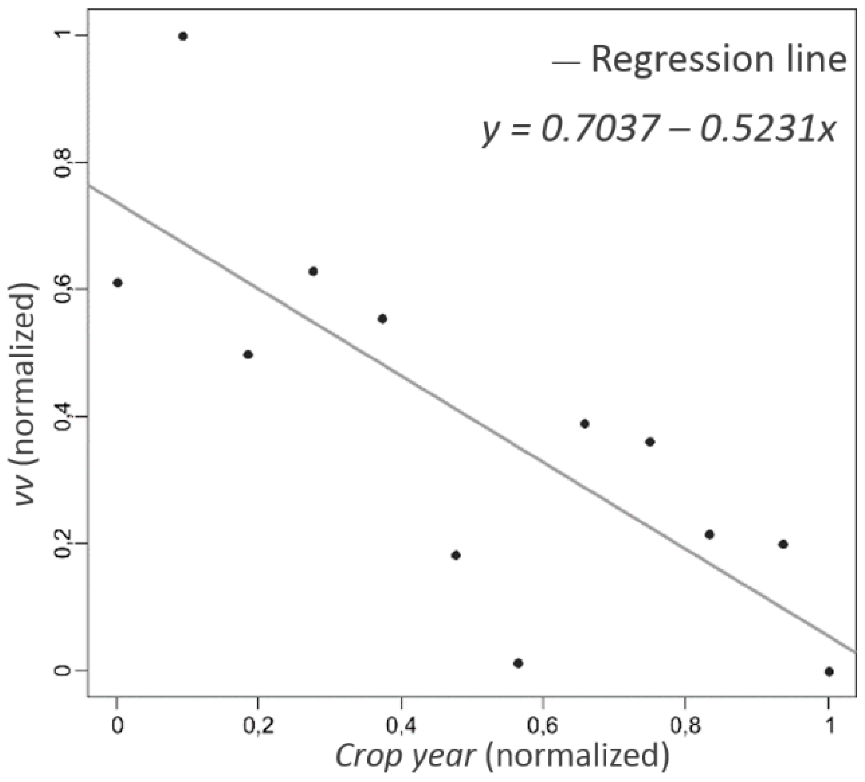
| vv | Vegetative vigor |
| bc | Boolean Criterion (bc) | nc | Numeric Criterion (nc) |
|---|---|---|---|
| bc1 | is maxyear greater than maxyear-1? | nc1 | (maxyear − maxyear-1)/maxyear-1 |
| bc2 | is maxyear greater than maxyear-2? | nc2 | (maxyear − maxyear-2)/maxyear-2 |
| bc3 | is minyear lesser than minyear-1? | nc3 | (minyear − minyear-1)/minyear-1 |
| bc4 | is minyear lesser than minyear-2? | nc4 | (minyear − minyear-2)/minyear-2 |
| bc5 | is ampyear greater than ampyear-1? | nc5 | (ampyear − ampyear-1)/ampyear-1 |
| bc6 | is ampyear greater than ampyear-2? | nc6 | (ampyear − ampyear-2)/ampyear-2 |
| bc7 | is guryear greater than guryear-1? | nc7 | (bgiyear − bgiyear-1)/iveyear-1 |
| bc8 | is guryear greater than guryear-2? | nc8 | (iveyear − iveyear-2)/iveyear-2 |
| bc9 | is ddpyear greater than ddpyear-1? | nc9 | ddsyear − dpsyear-1 |
| bc10 | is ddpyear greater than dppyear-2? | nc10 | ddsyear − dpsyear-2 |
| bc11 | is idpyear greater than idpyear-1? | nc11 | idpyear − ipsyear-1 |
| bc12 | is idpyear greater than idpyear-2? | nc12 | idpyear − ipsyear-2 |
| bc13 | is vvyear greater than vvyear-1? | nc13 | (ivvyear − ivvyear-1)/ivvyear-1 |
| bc14 | is vvyear greater than vvyear-2? | nc14 | (ivvyear − ivvyear-2)/ivvyear-2 |
| Pasture Status | 2011 | 2012 | Total | |||
|---|---|---|---|---|---|---|
| Samples | % | Samples | % | Samples | % | |
| Reformation | 52 | 14.1 | 52 | 12.6 | 104 | 13.3 |
| Renewal/Recovery | 50 | 13.6 | 49 | 11.9 | 99 | 12.7 |
| Reformation and Renewal/Recovery | 3 | 0.8 | 2 | 0.5 | 5 | 0.6 |
| In Degradation | 58 | 15.7 | 91 | 22.0 | 149 | 19.1 |
| Without Intervention | 206 | 55.8 | 219 | 53.0 | 425 | 54.3 |
| Total | 369 | 413 | 782 | |||
| Intervention/Degradation (EVI2 Time Series) | Stand (Field Assessment) | |||||
|---|---|---|---|---|---|---|
| Appropriate | Intermediate | Degraded | ||||
| Samples | % | Samples | % | Samples | % | |
| Reformation | 63 | 14.4 | 20 | 11.8 | 20 | 11.8 |
| Renewal/Recovery | 54 | 12.3 | 27 | 15.9 | 18 | 10.7 |
| Reformation and Renewal/Recovery | 4 | 0.9 | 1 | 0.6 | 0 | 0.0 |
| In Degradation | 80 | 18.2 | 30 | 17.6 | 34 | 20.1 |
| Without Intervention | 238 | 54.2 | 92 | 54.1 | 97 | 57.4 |
| Total | 439 | 170 | 169 | |||
| Pasture Status | Amazon | Cerrado | Atlantic Forest | Pantanal | ||||
|---|---|---|---|---|---|---|---|---|
| Samples | % | Samples | % | Samples | % | Samples | % | |
| Reformation | 31 | 11.6 | 53 | 13.6 | 18 | 17.0 | 2 | 10.0 |
| Renewal/Recovery | 38 | 14.2 | 46 | 11.8 | 12 | 11.3 | 3 | 15.0 |
| Reformation and Renewal/Recovery | 1 | 0.4 | 2 | 0.5 | 2 | 1.9 | 0 | 0.0 |
| In Degradation | 60 | 22.5 | 69 | 17.7 | 7 | 6.6 | 8 | 40.0 |
| Without Intervention | 137 | 51.3 | 219 | 56.3 | 67 | 63.2 | 7 | 35.0 |
| Total | 267 | 389 | 106 | 20 | ||||
© 2017 by the authors; licensee MDPI, Basel, Switzerland. This article is an open access article distributed under the terms and conditions of the Creative Commons Attribution (CC-BY) license (http://creativecommons.org/licenses/by/4.0/).
Share and Cite
Aguiar, D.A.; Mello, M.P.; Nogueira, S.F.; Gonçalves, F.G.; Adami, M.; Rudorff, B.F.T. MODIS Time Series to Detect Anthropogenic Interventions and Degradation Processes in Tropical Pasture. Remote Sens. 2017, 9, 73. https://doi.org/10.3390/rs9010073
Aguiar DA, Mello MP, Nogueira SF, Gonçalves FG, Adami M, Rudorff BFT. MODIS Time Series to Detect Anthropogenic Interventions and Degradation Processes in Tropical Pasture. Remote Sensing. 2017; 9(1):73. https://doi.org/10.3390/rs9010073
Chicago/Turabian StyleAguiar, Daniel Alves, Marcio Pupin Mello, Sandra Furlan Nogueira, Fabio Guimarães Gonçalves, Marcos Adami, and Bernardo Friedrich Theodor Rudorff. 2017. "MODIS Time Series to Detect Anthropogenic Interventions and Degradation Processes in Tropical Pasture" Remote Sensing 9, no. 1: 73. https://doi.org/10.3390/rs9010073