
Is Spatial Resolution Critical in Urbanization Velocity Analysis? Investigations in the Pearl River Delta


Abstract
:
1. Introduction
2. Study Areas and Data Collection
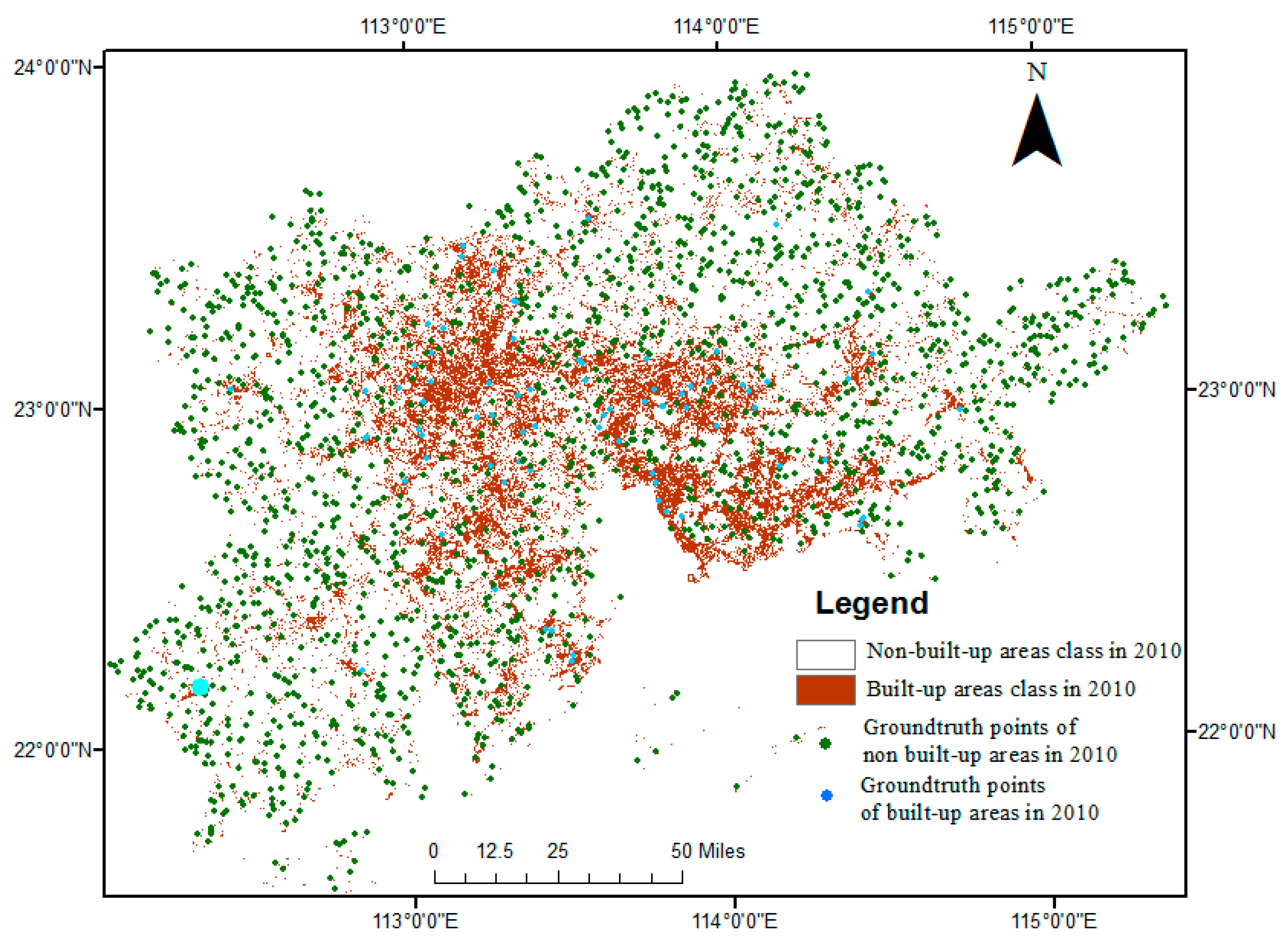
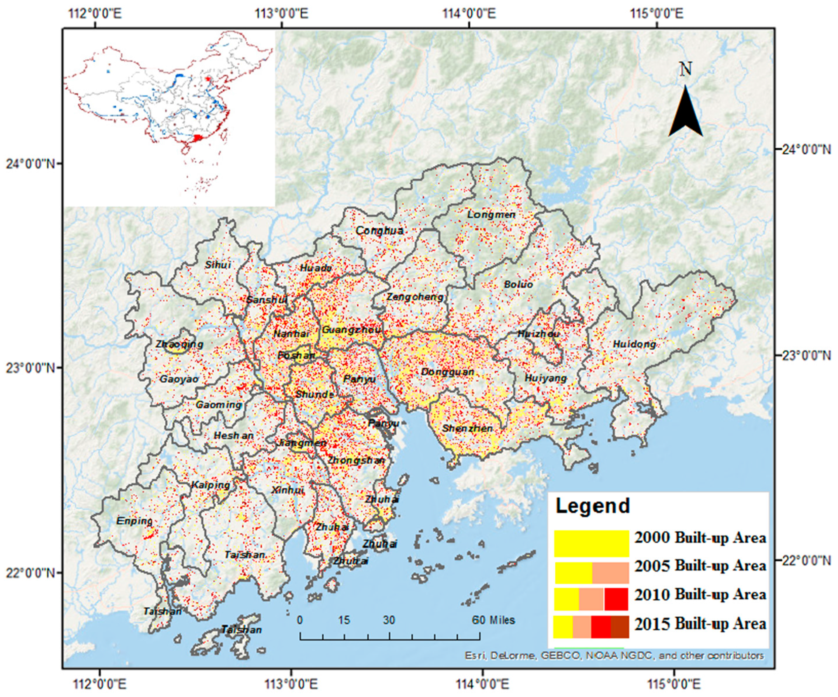
2.1. Study Area
2.2. Data Collection
3. Methodology
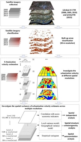
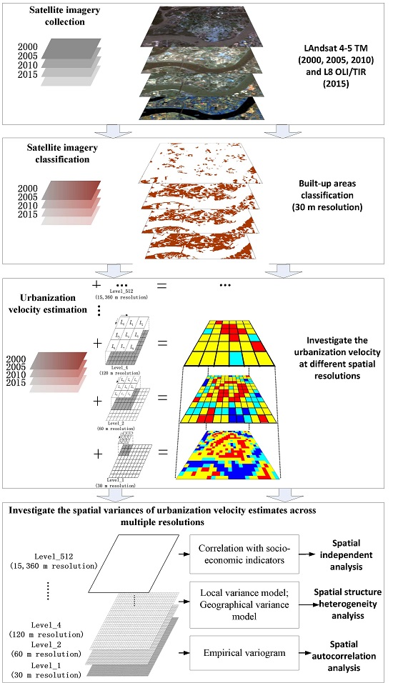
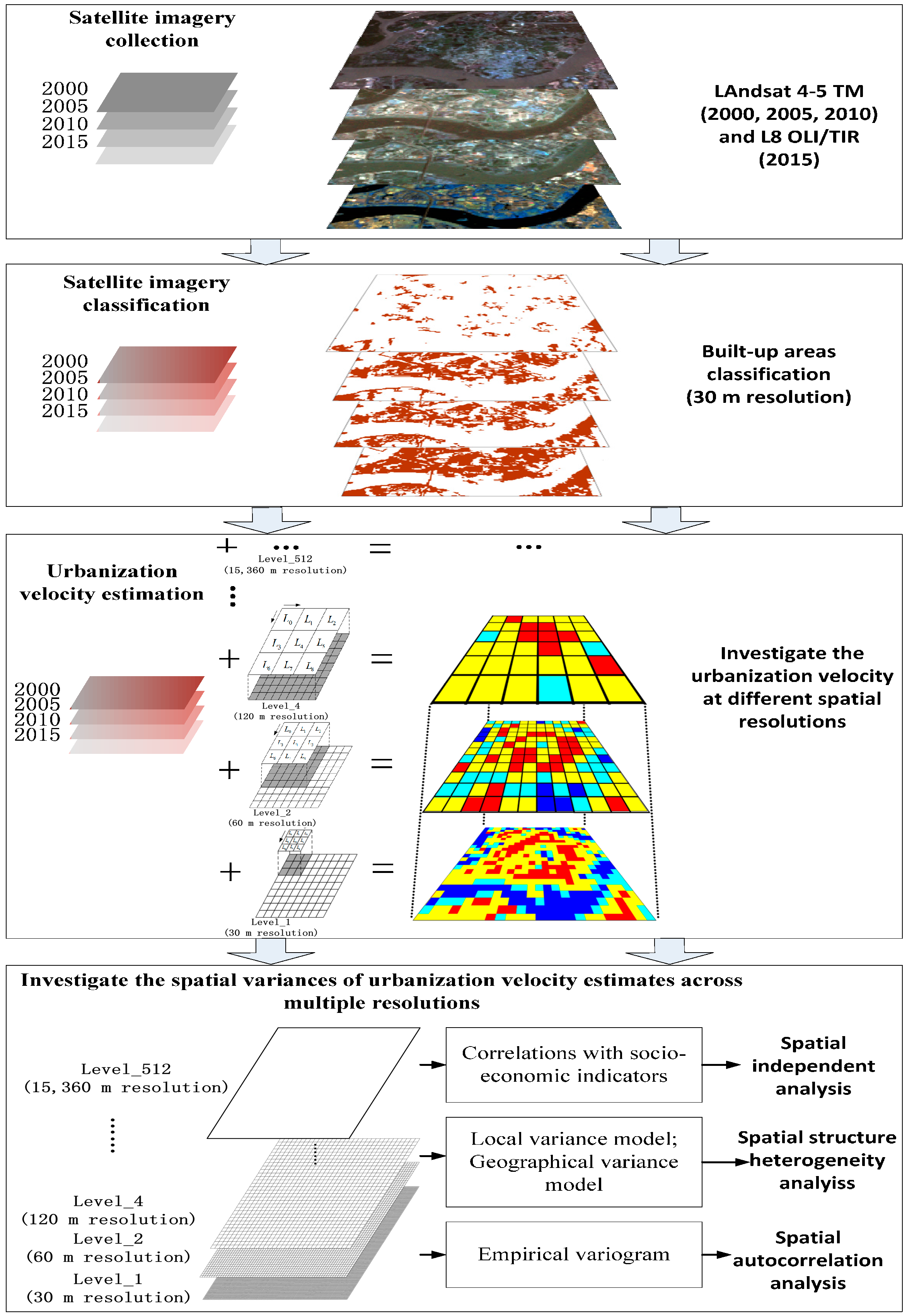
3.1. Workflow
3.2. Land Use and Land Cover Classification
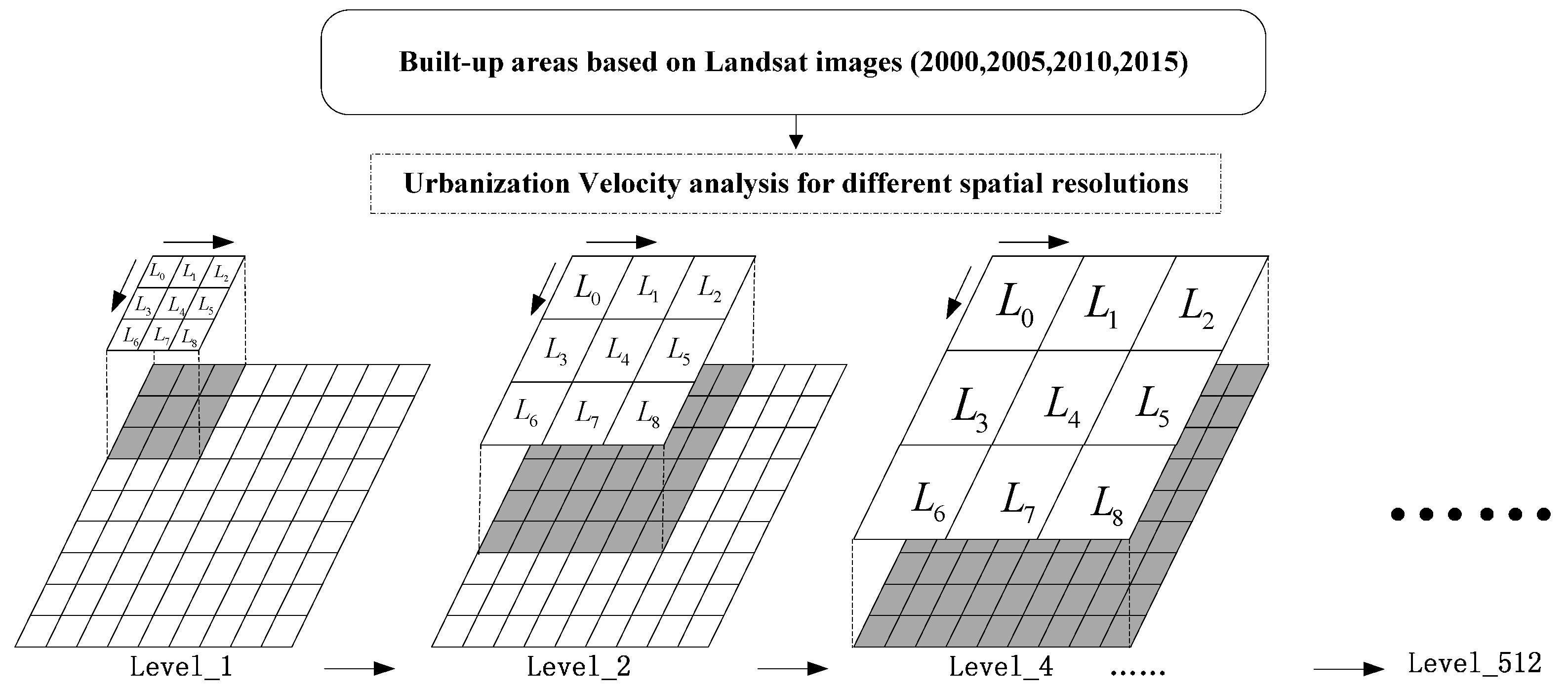
3.3. Urbanization Velocity Estimation at Different Spatial Resolutions
3.4. Statistical Test for the Dependence of Urbanization Velocity on Spatial Resolution
3.5. Quantitative Descriptions of Spatial Resolution Domains and Thresholds
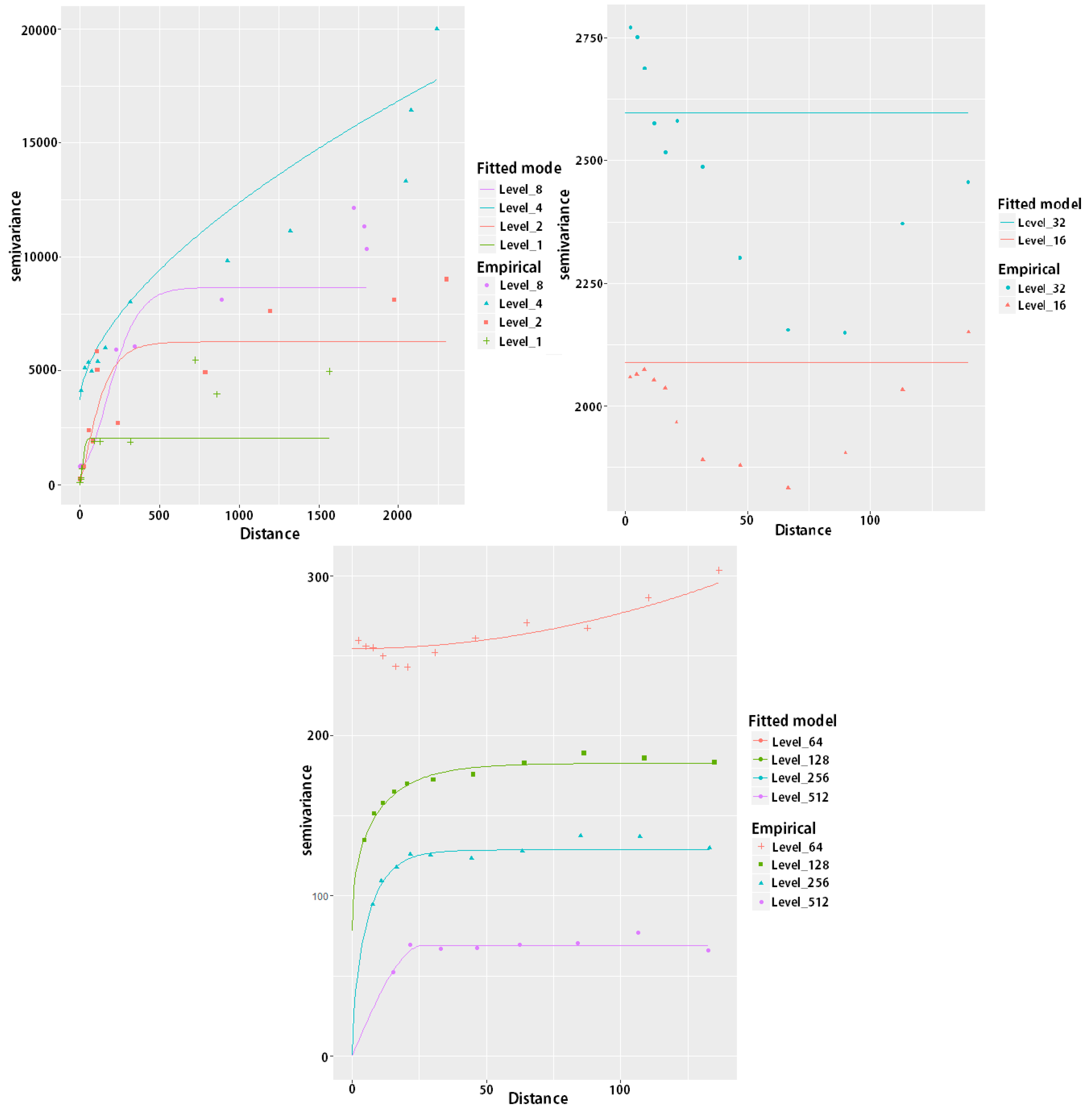
3.5.1. Empirical Variogram Method
3.5.2. Local Variance Method
3.5.3. Geographic Variance Method
4. Results
4.1. Land Use/Land Cover Accuracy
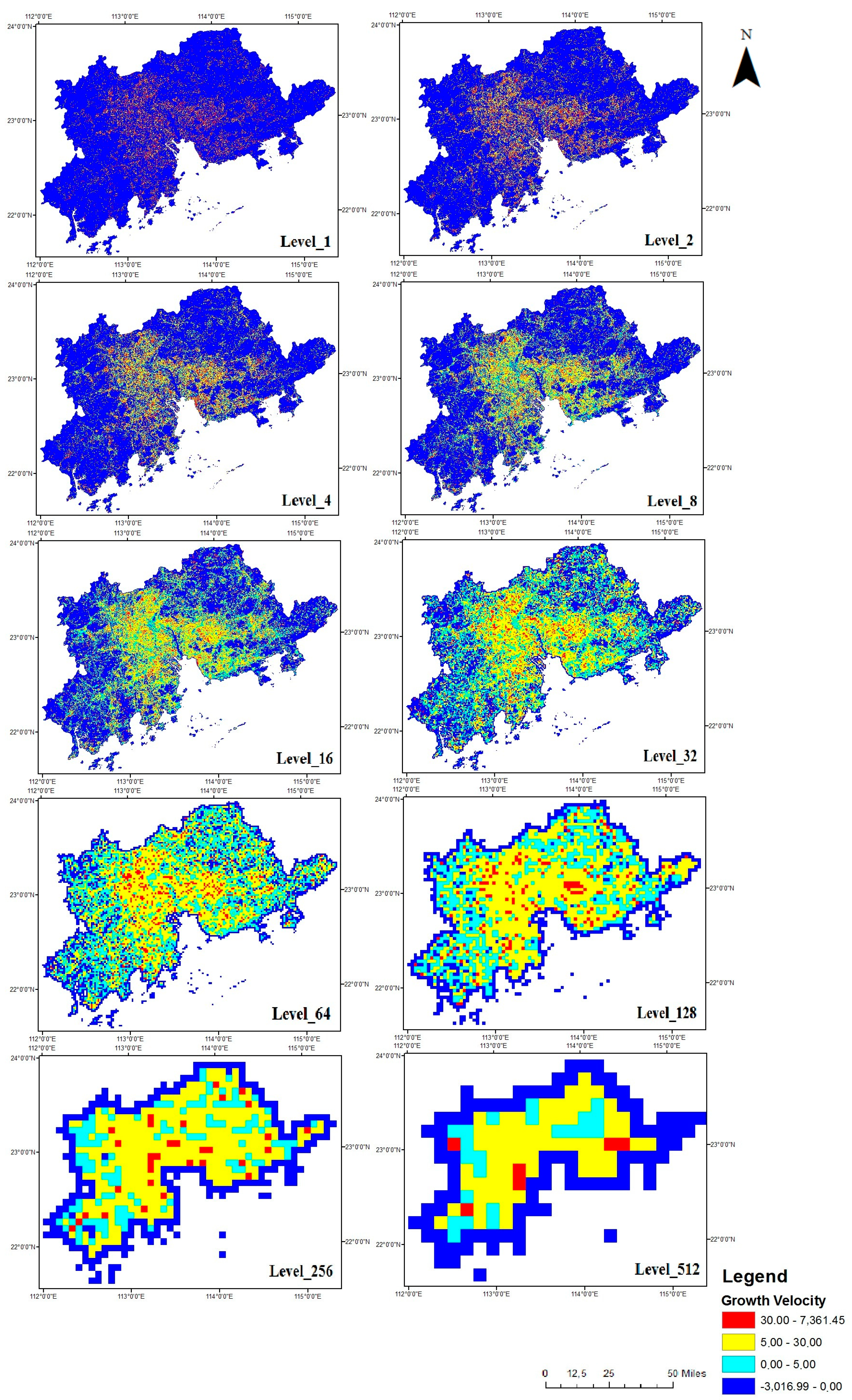
4.2. Multi-Scale Urbanization Velocity
4.3. Lack of Scale–Dependence in Urbanization Velocity (UV) Estimations
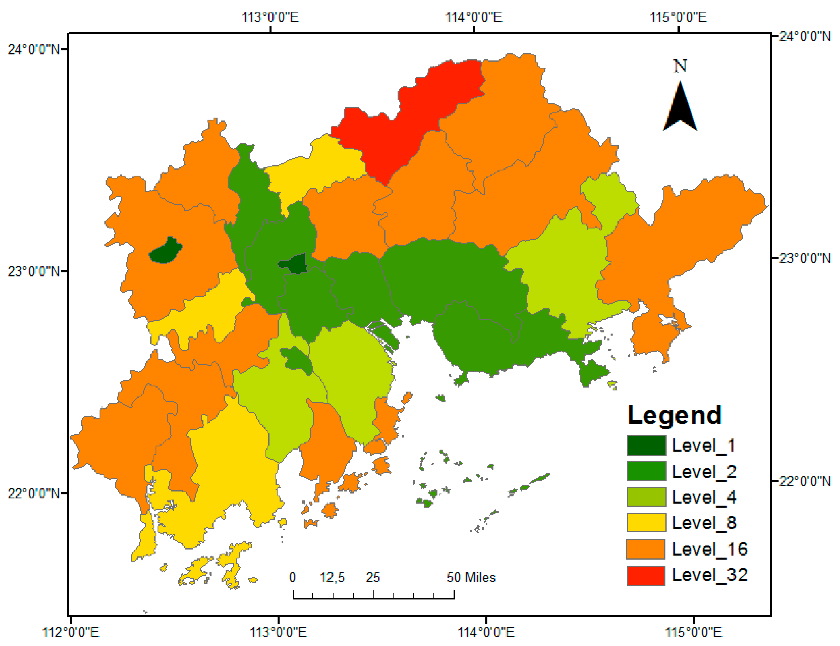
4.4. Spatial Autocorrelation and Spatial Variability of UV Analysis Results Based on Different Spatial Resolutions
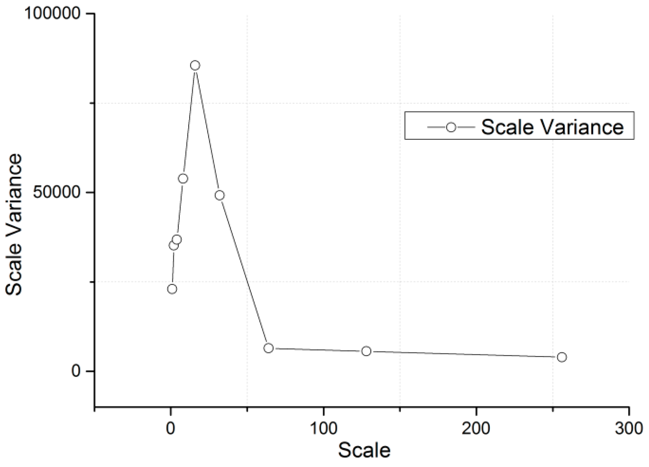
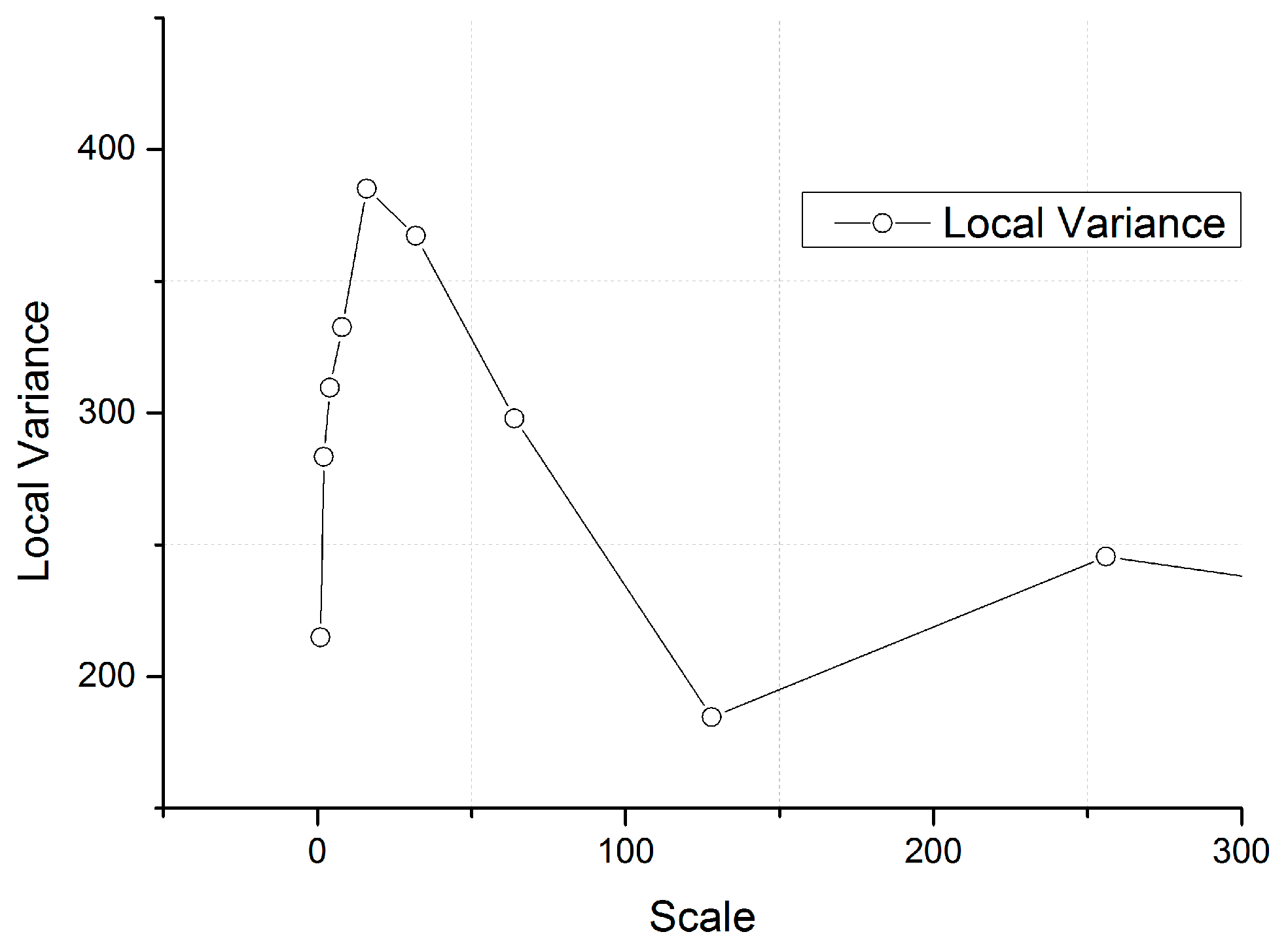
4.5. Local Variance and Geographical Variance Of the UV Analysis Results at Different Spatial Resolutions
5. Discussion
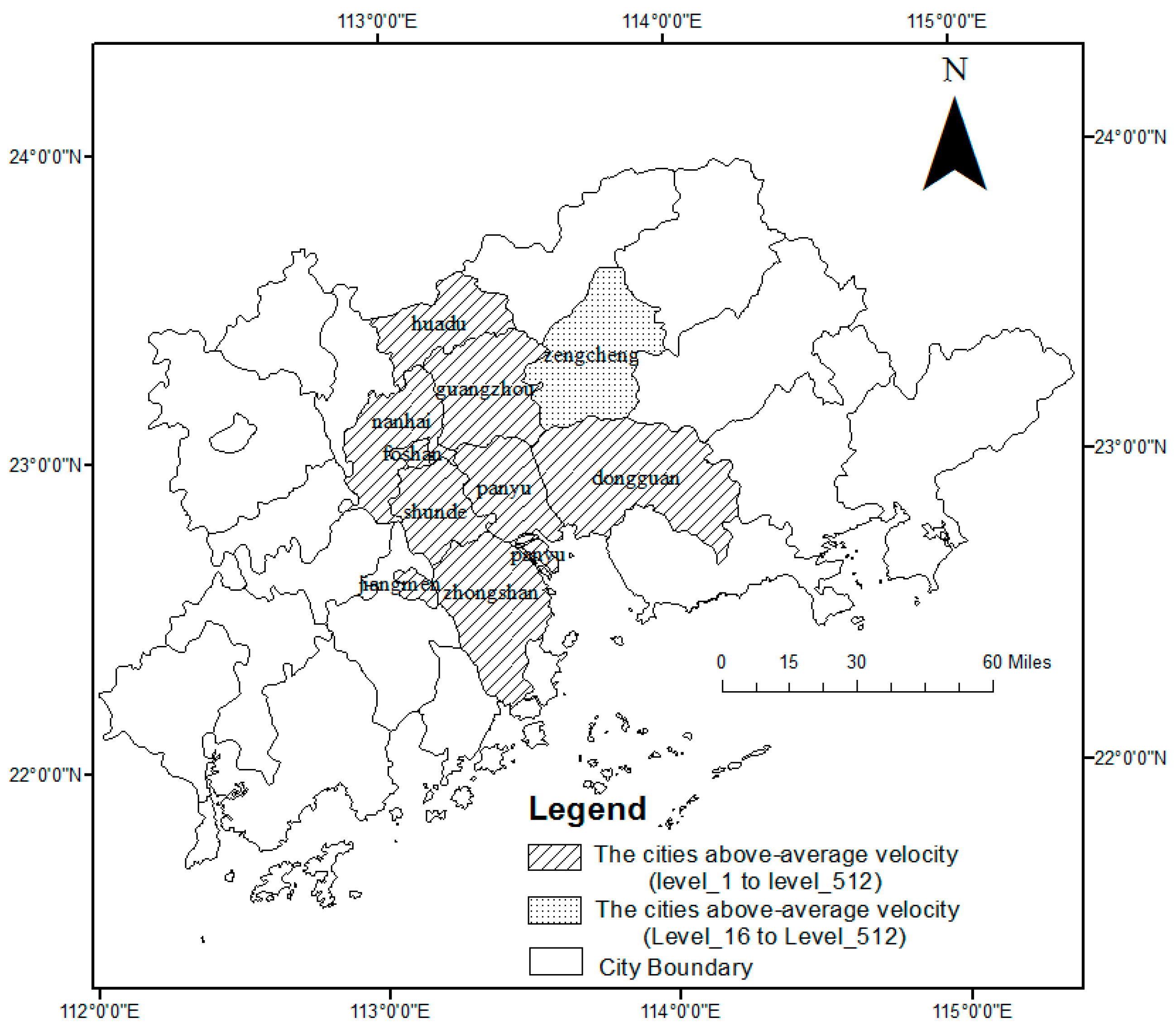
5.1. Scale-Independence in the City-Based Urbanization Velocity Analysis Results
5.2. Spatial Variances of the Multi-Resolution Urbanization Velocity Analysis Results
6. Conclusions and Outlook
Acknowledgments
Author Contributions
Conflicts of Interest
References
- United Nations. World Urbanization Prospects: The 2014 Revision: Highlights; ST/ESA/SER.A/352; United Nations: New York, NY, USA, 2014; pp. 1–200. [Google Scholar]
- Zhang, Q.; Seto, K.C. Mapping urbanization dynamics at regional and global scales using multi-temporal DMSP/OLS nighttime light data. Remote Sens. Environ. 2011, 115, 2320–2329. [Google Scholar] [CrossRef]
- Xu, C.; Wang, S.; Zhou, Y.; Wang, L.; Liu, W. A comprehensive quantitative evaluation of new sustainable urbanization level in 20 Chinese urban agglomerations. Sustainability 2016, 8, 91. [Google Scholar] [CrossRef]
- Liu, Y.Q.; Xu, J.P.; Luo, H.W. An integrated approach to modelling the economy-society-ecology system in urbanization process. Sustainability 2014, 6, 1946–1972. [Google Scholar] [CrossRef]
- Bekele, H. Urbanization and Urban Sprawl. Master’s Thesis, Royal Institute of Technology, Stockholm, Sweden, April 2005. [Google Scholar]
- McIntyre, N.E. Ecology of urban arthropods: A review and a call to action. Ann. Entomol. Soc. Am. 2000, 93, 825–835. [Google Scholar] [CrossRef]
- United Nations Population Division. World Population Prospects: The 2002 Revision: Highlights; ESA/P/WP. 180; United Nations: New York, NY, USA, 2002; pp. 100–200. [Google Scholar]
- Schneider, A.; Woodcock, C.E. Compact, dispersed, fragmented, extensive? A comparison of urban growth in twenty-five global cities using remotely sensed data, pattern metrics and census information. Urban Stud. 2008, 45, 659–692. [Google Scholar] [CrossRef]
- Angel, S.; Parent, J.; Civco, D.L.; Blei, A.M. Atlas of Urban Expansion; Lincoln Institute of Land Policy: Cambridge, MA, USA, 2012; pp. 10–50. [Google Scholar]
- Angel, S.; Sheppard, S.; Civco, D.L.; Buckley, R.; Chabaeva, A.; Gitlin, L.; Kraley, A.; Parent, J.; Perlin, M. The Dynamics of Global Urban Expansion; World Bank, Transport and Urban Development Department: Washington, DC, USA, 2005; pp. 205–220. [Google Scholar]
- Ewing, R. Is LOS angeles-style sprawl desirable? J. Am. Plan. Assoc. 1997, 63, 107–126. [Google Scholar] [CrossRef]
- Burchell, R.W.; Shad, N.A.; Listokin, D.; Phillips, H.; Downs, A.; Seskin, S.; Davis, J.S.; Moore, T.; Helton, D.; Gall, M. The Costs of Sprawl-Revisited; (No. Project H-10 FY’95); National Academy Press: Washington, DC, USA, 1998; pp. 1–200. [Google Scholar]
- Frenkel, A.; Ashkenazi, M. Measuring urban sprawl: How can we deal with it? Environ. Plan. B Plan. Des. 2008, 35, 56–79. [Google Scholar] [CrossRef]
- Wissen Hayek, U.; Jaeger, J.A.G.; Schwick, C.; Jarne, A.; Schuler, M. Measuring and Assessing Urban Sprawl: What are the Remaining Options for Future Settlement Development in Switzerland for 2030? Appl. Spat. Anal. 2030, 4, 249–279. [Google Scholar] [CrossRef] [Green Version]
- Herold, M.; Goldstein, N.C.; Clarke, K.C. The spatiotemporal form of urban growth: Measurement, analysis and modeling. Remote Sens. Environ. 2003, 86, 286–302. [Google Scholar] [CrossRef]
- Ji, W.; Ma, J.; Twibell, R.W.; Underhill, K. Characterizing urban sprawl using multi-stage remote sensing images and landscape metrics. Comput. Environ. Urban Syst. 2006, 30, 861–879. [Google Scholar] [CrossRef]
- Rumor, M.; Coors, V.; Fendel, E.M.; Zlatanova, S. Urban and Regional Data Management: UDMS 2007 Annual; CRC Press: Boca Raton, FL, USA, 2007; pp. 3–50. [Google Scholar]
- Liu, H.; Weng, Q. Landscape metrics for analysing urbanization-induced land use and land cover changes. Geocarto Int. 2013, 28, 582–593. [Google Scholar] [CrossRef]
- Liu, Z.; He, C.; Wu, J. General spatiotemporal patterns of urbanization: An examination of 16 World cities. Sustainability 2016, 8, 41–56. [Google Scholar] [CrossRef]
- Sharmeen, F.; Arentze, T.; Timmermans, H. Dynamics of face-to-face social interaction frequency: Role of accessibility, urbanization, changes in geographical distance and path dependence. J. Transp. Geogr. 2014, 4, 211–220. [Google Scholar] [CrossRef]
- Lee, E. Designing service coverage and measuring accessibility and serviceability of rural and small urban ambulance systems. Systems 2014, 2, 34–53. [Google Scholar] [CrossRef]
- Maktav, D.; Sunar Erbek, F.; Jurgens, C. Remote sensing of urban areas. Int. J. Remote Sens. 2005, 26, 655–659. [Google Scholar] [CrossRef]
- Taubenböck, H.; Esch, T.; Felbier, A.; Wiesner, M.; Roth, A.; Dech, S. Monitoring urbanization in mega cities from space. Remote Sens. Environ. 2012, 117, 162–176. [Google Scholar] [CrossRef]
- Taubenböck, H.; Wiesner, M.; Felbier, A.; Marconcini, M.; Esch, T.; Dech, S. New dimensions of urban landscapes: The spatio-temporal evolution from a polynuclei area to a mega-region based on remote sensing data. Appl. Geogr. 2014, 47, 137–153. [Google Scholar] [CrossRef]
- Zhang, J.; Liu, J.; Zhai, L.; Hou, W. Implementation of geographical conditions monitoring in Beijing-Tianjin-Hebei, China. ISPRS Int. J. Geo-Inf. 2016, 5, 89–115. [Google Scholar] [CrossRef]
- Li, X.; Yeh, A.G.O. Analyzing spatial restructuring of land use patterns in a fast growing region using remote sensing and GIS. Landsc. Urban Plan. 2004, 69, 335–354. [Google Scholar] [CrossRef]
- Bhatta, B.; Saraswati, S.; Bandyopadhyay, D. Quantifying the degree-of-freedom, degree-of-sprawl, and degree-of-goodness of urban growth from remote sensing data. Appl. Geogr. 2010, 30, 96–111. [Google Scholar] [CrossRef]
- Kong, F.; Nakagoshi, N. Spatial-temporal gradient analysis of urban green spaces in Jinan, China. Landsc. Urban Plan. 2006, 78, 147–164. [Google Scholar] [CrossRef]
- Zhou, X.; Wang, Y.C. Spatial–temporal dynamics of urban green space in response to rapid urbanization and greening policies. Landsc. Urban Plan. 2011, 100, 268–277. [Google Scholar] [CrossRef]
- Ma, T.; Yin, Z.; Li, B.; Zhou, C.; Haynie, S. Quantitative estimation of the velocity of urbanization in China using nighttime luminosity data. Remote Sens. 2016, 8, 94–118. [Google Scholar] [CrossRef]
- Braak, C.J.F.T.; Prentice, I.C. A theory of gradient analysis. Adv. Ecol. Res. 1988, 18, 271–317. [Google Scholar]
- McDonnell, M.J.; Hahs, A.K. The use of gradient analysis studies in advancing our understanding of the ecology of urbanizing landscapes: current status and future directions. Landsc. Ecol. 2008, 23, 1143–1155. [Google Scholar] [CrossRef]
- Zhang, Z.; Tu, Y.; Li, X. Quantifying the spatiotemporal patterns of urbanization along urban-rural gradient with a roadscape transect approach: A case study in Shanghai, China. Sustainability 2016, 8, 862–882. [Google Scholar] [CrossRef]
- Li, Q.; Lu, L.; Weng, Q.; Xie, Y.; Guo, H. Monitoring urban dynamics in the southeast USA using time-series DMSP/OLS nightlight imagery. Remote Sens. 2016, 8, 578–594. [Google Scholar] [CrossRef]
- Timm, S.; Frydenberg, M.; Janson, C.; Campbell, B.; Forsberg, B.; Gislason, T.; Holm, M.; Jogi, R. The urban-rural gradient in asthma: A popluation-based study in Northen Europe. Int. J. Environ. Res. Public Health 2015, 13, 93–115. [Google Scholar] [CrossRef] [PubMed]
- Li, G.; Zhang, P.; Wei, G.; Xie, Y.; Yu, X.; Long, X. Multiple-point temperature gradient algorithm for ring laser gyroscope bias compensation. Sensors 2015, 15, 29910–29922. [Google Scholar] [CrossRef] [PubMed]
- Bhatta, B. Analysis of urban growth pattern using remote sensing and GIS: A case study of Kolkata, India. Int. J. Remote Sens. 2009, 30, 4733–4746. [Google Scholar] [CrossRef]
- Singh, G.K.; Siahpush, M. Increasing rural–urban gradients in US suicide mortality, 1970–1997. Am. J. Public Health 2002, 92, 1161–1167. [Google Scholar] [CrossRef] [PubMed]
- McDonnell, M.J.; Pickett, S.T.A. Ecosystem structure and function along urban-rural gradients: an unexploited opportunity for ecology. Ecology 1990, 71, 1232–1237. [Google Scholar] [CrossRef]
- Jenerette, G.D.; Harlan, S.L.; Brazel, A.; Jones, N.; Larsen, L.; Stefanov, W.L. Regional relationships between surface temperature, vegetation, and human settlement in a rapidly urbanizing ecosystem. Landsc. Ecol. 2006, 22, 353–365. [Google Scholar] [CrossRef]
- Crooks, K.R.; Suarez, A.V.; Bolger, D.T. Avian assemblages along a gradient of urbanization in a highly fragmented landscape. Biol. Conserv. 2004, 115, 451–462. [Google Scholar] [CrossRef]
- Zhang, L.; Wu, J.; Zhen, Y.; Shu, J. RETRACTED: A GIS-based gradient analysis of urban landscape pattern of Shanghai metropolitan area, China. Landsc. Urban Plan. 2004, 69, 1–16. [Google Scholar] [CrossRef]
- Hahs, A.K.; McDonnell, M.J. Selecting independent measures to quantify Melbourne’s urban–rural gradient. Landsc. Urban Plan. 2006, 78, 435–448. [Google Scholar] [CrossRef]
- Solon, J. Spatial context of urbanization: Landscape pattern and changes between 1950 and 1990 in the Warsaw metropolitan area, Poland. Landsc. Urban Plan. 2009, 93, 250–261. [Google Scholar] [CrossRef]
- Trivedi, M.R.; Berry, P.M.; Morecroft, M.D.; Dawson, T.P. Spatial scale affects bioclimate model projections of climate change impacts on mountain plants. Glob. Chang. Biol. 2008, 14, 1089–1103. [Google Scholar] [CrossRef]
- Loarie, S.R.; Duffy, P.B.; Hamilton, H.; Asner, G.P.; Field, C.B.; Ackerly, D.D. The velocity of climate change. Nature 2009, 462, 1052–1055. [Google Scholar] [CrossRef] [PubMed]
- Jokimäki, J.; Kaisanlahti-Jokimäki, M.L.; Sorace, A.; Fernández-Juricic, E.; Rodriguez-Prieto, I.; Jimenez, M.D. Evaluation of the ‘safe nesting zone’ hypothesis across an urban gradient: A multi-scale study. Ecography 2005, 28, 59–70. [Google Scholar] [CrossRef]
- Lillesand, T.; Kiefer, R.W.; Chipman, J. Remote Sensing and Image Interpretation; John Wiley & Sons: Hoboken, NJ, USA, 2014; pp. 5–200. [Google Scholar]
- Woodcock, C.E.; Strahler, A.H.; Jupp, D.L.B. The use of variograms in remote sensing: II. Real digital images. Remote Sens. Environ. 1988, 25, 349–379. [Google Scholar] [CrossRef]
- Drǎguţ, L.; Tiede, D.; Levick, S.R. ESP: A tool to estimate scale parameter for multiresolution image segmentation of remotely sensed data. Int. J. Geogr. Inf. Sci. 2010, 24, 859–871. [Google Scholar] [CrossRef]
- Wu, H.; Li, Z.L. Scale issues in remote sensing: A review on analysis, processing and modeling. Sensors 2009, 9, 1768–1793. [Google Scholar] [CrossRef] [PubMed]
- Moellering, H.; Tobler, W. Geographical variances. Geogr. Anal. 1972, 4, 34–50. [Google Scholar] [CrossRef]
- Garrigues, S.; Allard, D.; Baret, F.; Weiss, M. Quantifying spatial heterogeneity at the landscape scale using variogram models. Remote Sens. Environ. 2006, 103, 81–96. [Google Scholar] [CrossRef]
- Tarnavsky, E.; Garrigues, S.; Brown, M.E. Multiscale geostatistical analysis of AVHRR, SPOT-VGT, and MODIS global NDVI Products. Remote Sens. Environ. 2008, 112, 535–549. [Google Scholar] [CrossRef]
- Brown, G.; Michon, G.; Peyrière, J. On the multifractal analysis of measures. J. Stat. Phys. 1992, 66, 775–790. [Google Scholar] [CrossRef]
- Lopes, R.; Betrouni, N. Fractal and multifractal analysis: A review. Med. Image Anal. 2009, 13(4), 634–649. [Google Scholar] [CrossRef] [PubMed]
- Hu, Z.; Chen, Y.; Islam, S. Multiscaling properties of soil moisture images and decomposition of large- and small-scale features using wavelet transforms. Int. J. Remote Sens. 1998, 19, 2451–2467. [Google Scholar] [CrossRef]
- Keitt, T.H.; Urban, D.L. Scale-specific inference using wavelets. Ecology 2005, 86, 2497–2504. [Google Scholar] [CrossRef]
- Beer, R. Remote Sensing by Fourier Transform Spectrometry; John Wiley & Sons: Toronto, ON, Canada, 1992; pp. 1–45. [Google Scholar]
- Kunttu, I.; Lepisto, L.; Rauhamaa, J.; Visa, A. Multiscale fourier descriptor for shape-based image retrieval. In Proceedings of the 17th International Conference on Pattern Recognition, Cambridge, UK, 23–26 August 2004; pp. 765–768.
- Atkinson, P.M.; Aplin, P. Spatial variation in land cover and choice of spatial resolution for remote sensing. Int. J. Remote Sens. 2004, 25, 3687–3702. [Google Scholar] [CrossRef]
- Woodcock, C.E.; Strahler, A.H. The factor of scale in remote sensing. Remote Sens. Environ. 1987, 21, 311–332. [Google Scholar] [CrossRef]
- Marceau, D.J.; Gratton, D.J.; Fournier, R.A.; Fortin, J.P. Remote-sensing and the measurement of geographical entities in a forested environment. 2. The optimal spatial-resolution. Remote Sens. Environ. 1994, 49, 105–117. [Google Scholar] [CrossRef]
- Atkinson, P.M.; Curran, P.J. Defining an optimal size of support for remote sensing investigations. IEEE Trans. Geosci. Remote Sens. 1995, 33, 768–776. [Google Scholar] [CrossRef]
- Curran, P.J.; Atkinson, P.M. Geostatistics and remote sensing. Prog. Phys. Geogr. 1998, 22, 61–78. [Google Scholar] [CrossRef]
- Taubenböck, H.; Wiesner, M. The spatial network of megaregions-Types of connectivity between cities based on settlement patterns derived from EO-data. Comput. Environ. Urban Syst. 2015, 54, 65–180. [Google Scholar] [CrossRef]
- United States Geological Survey. Using the USGS Landsat 8 Product. Available online: https://landsat.usgs.gov/using-usgs-landsat-8-product (accessed on 10 July 2016).
- Blaschke, T. Object based image analysis for remote sensing. ISPRS J. Photogramm. Remote Sens. 2010, 65, 2–16. [Google Scholar] [CrossRef]
- Wei, C.; Taubenböck, H.; Blaschke, T. Measuring urban agglomeration using a city-scale dasymetric population map: A study in the Pearl River Delta, China. Habitat Int. 2017, 59, 32–43. [Google Scholar] [CrossRef]
- Drăguţ, L.; Csillik, O.; Eisank, C.; Tiede, D. Automated parameterisation for multi-scale image segmentation on multiple layers. ISPRS J. Photogramm. Remote Sens. 2014, 88, 119–127. [Google Scholar] [CrossRef] [PubMed]
- Hofmann, P.; Blaschke, T.; Strobl, J. Quantifying the robustness of fuzzy rule sets in object-based image analysis. Int. J. Remote Sens. 2011, 32, 7359–7381. [Google Scholar] [CrossRef]
- Benz, U.C.; Hofmann, P.; Willhauck, G.; Lingenfelder, I.; Heynen, M. Multi-resolution, object-oriented fuzzy analysis of remote sensing data for GIS-ready information. ISPRS J. Photogramm. Remote Sens. 2004, 58, 239–258. [Google Scholar] [CrossRef]
- Burrough, P.A.; McDonnell, R.A.; McDonnell, R.; Lloyd, C.D. Principles of Geographical Information Systems; Oxford University Press: Oxford, UK, 2015; pp. 10–19. [Google Scholar]
- Townshend, J.R. The spatial resolving power of earth resources satellites: A review. Prog. Phys. Geogr. 1980, 5, 1–36. [Google Scholar] [CrossRef]
- Delhomme, J.P. Spatial variability and uncertainty in groundwater flow parameters: A geostatistical approach. Water Resour. Res. 1979, 15, 269–280. [Google Scholar] [CrossRef]
- Wilson, E.H.; Hurd, J.D.; Civco, D.L.; Prisloe, M.P.; Arnold, C. Development of a geospatial model to quantify describe and map urban growth. Remote Sens. Environ. 2004, 86, 275–285. [Google Scholar] [CrossRef]
- Goodchild, M.; Quattrochi, D. Scale in Remote Sensing and GIS; CRC Press: Boca Raton, FL, USA, 1997; p. 406. [Google Scholar]
- Wu, J.; Jelinski, D.E.; Luck, M.; Tueller, P.T. Multiscale analysis of landscape heterogeneity: Scale variance and pattern metrics. Geogr. Inf. Sci. 2000, 6, 6–19. [Google Scholar] [CrossRef] [PubMed]
- Woodcock, C.E.; Strahler, A.H.; Jupp, D.L.B. The use of variograms in remote sensing: I. Scene models and simulated images. Remote Sens. Environ. 1988, 25, 323–348. [Google Scholar] [CrossRef]
- Phinn, S.R.; Menges, C.; Hill, G.J.E.; Stanford, M. Optimizing remotely sensed solutions for monitoring, modeling, and managing coastal environments. Remote Sens. Environ. 2000, 73, 117–132. [Google Scholar] [CrossRef]
- Arlinghaus, S.L.; Kerski, J.J. Spatial Mathematics: Theory and Practice through Mapping; CRC Press: Boca Raton, FL, USA, 2013; pp. 155–174. [Google Scholar]
- Munda, G. Social multi-criteria evaluation for urban sustainability policies. Land Use Policy 2006, 23, 86–94. [Google Scholar] [CrossRef]
- Wang, J.; Ge, Y.; Heuvelink, G.B.M.; Zhou, C. Upscaling in situ soil moisture observations to pixel averages with spatio-temporal geostatistics. Remote Sens. 2015, 7, 11372–11388. [Google Scholar] [CrossRef]
- Neumann, C.; Weiss, G.; Schmidtlein, S.; Itzerott, S.; Lausch, A.; Doktor, D.; Brell, M. Gradient-based assessment of habitat quality for spectral ecosystem monitoring. Remote Sens. 2015, 7, 2871–2898. [Google Scholar] [CrossRef]
- Treitz, P.; Howarth, P. High spatial resolution remote sensing data for forest ecosystem classification: an examination of spatial scale. Remote Sens. Environ. 2000, 72, 268–289. [Google Scholar] [CrossRef]
- Hyppänen, H. Spatial autocorrelation and optimal spatial resolution of optical remote sensing data in boreal forest environment. Int. J. Remote Sens. 1996, 7, 3441–3452. [Google Scholar] [CrossRef]
- Coops, N.; Culvenor, D. Utilizing local variance of simulated high spatial resolution imagery to predict spatial pattern of forest stands. Remote Sens. Environ. 2000, 71, 248–260. [Google Scholar] [CrossRef]
- Nagendra, H. Using remote sensing to assess biodiversity. Int. J. Remote Sens. 2001, 22, 2377–2400. [Google Scholar] [CrossRef]
- Cohen, W.B.; Goward, S.N. Landsat’s role in ecological applications of remote sensing. BioScience 2004, 54, 535–545. [Google Scholar] [CrossRef]
- Spielman, S.E.; Yoo, E. The spatial dimensions of neighborhood effects. Soc. Sci. Med. 2009, 68, 1098–1105. [Google Scholar] [CrossRef] [PubMed]
- Moellering, H. The scope and conceptual content of analytical cartography. Cartogr. Geogr. Inf. Sci. 2000, 27, 205–224. [Google Scholar] [CrossRef]
- Wei, C.; Cabrera-Barona, P.; Blaschke, T. Local geographic variation of public services inequality: does the neighborhood scale matter? Int. J. Environ. Res. Public. Health 2016, 13, 981–998. [Google Scholar] [CrossRef] [PubMed]
- Ramachandra, T.V.; Aithal, B.H.; Sanna, D.D. Insights to urban dynamics through landscape spatial pattern analysis. Int. J. Appl. Earth Obs. Geoinf. 2012, 18, 329–343. [Google Scholar]
- Salvati, L.; Zitti, M. Monitoring vegetation and land use quality along the rural–urban gradient in a Mediterranean region. Appl. Geogr. 2012, 32, 896–903. [Google Scholar] [CrossRef]
- Weng, Q.; Quattrochi, D.A. Urban Remote Sensing; CRC Press: Boca Raton, FL, USA, 2006; pp. 3–10. [Google Scholar]
- Weng, Q.; Lu, D. A sub-pixel analysis of urbanization effect on land surface temperature and its interplay with impervious surface and vegetation coverage in Indianapolis, United States. Int. J. Appl. Earth Obs. Geoinf. 2008, 10, 68–83. [Google Scholar] [CrossRef]
- Jiang, Y.; Fu, P.; Weng, Q. Assessing the impacts of urbanization-associated land use/cover change on land surface temperature and surface moisture: A case study in the midwestern United States. Remote Sens. 2015, 7, 4880–4898. [Google Scholar] [CrossRef]


| (Path, Row) | (121,44) | (121,45) | (122,43) | (122,44) | (122,45) | (123,43) | (123,44) | (123,45) | |
|---|---|---|---|---|---|---|---|---|---|
| Year | |||||||||
| 2000 | 15 September | 15 September | 21 August | 21 August | 21 August | 8 October | 8 October | 13 September | |
| 2005 | 12 August | 12 August | 18 July | 18 July | 18 July | 11 September | 11 September | 11 September | |
| 2010 | 29 October | 29 October | 18 September | 18 September | 18 September | 7 July | 7 July | 7 July | |
| 2015 | 8 August | 8 August | 18 October | 18 October | 18 October | 6 August | 6 August | 22 August | |
| 2000 | Reference Built-Up Areas | Reference Non-Built-Up Areas | Ground Truth Total |
| Built-up areas | 91 | 50 | 141 |
| Non-built-up areas | 103 | 1756 | 1859 |
| Total | 194 | 1806 | 2000 |
| Overall accuracy | 0.9235 | ||
| 2005 | Reference Built-Up Areas | Reference Non-Built-Up Areas | Ground Truth Total |
| Built-up areas | 143 | 128 | 271 |
| Non-built-up areas | 80 | 1649 | 1729 |
| Total | 223 | 1777 | 2000 |
| Overall | 0.8960 | ||
| 2010 | Reference Built-Up Areas | Reference Non-Built-Up Areas | Ground Truth Total |
| Built-up areas | 167 | 88 | 255 |
| Non-built-up areas | 103 | 1642 | 1745 |
| Total | 270 | 1730 | 2000 |
| Overall accuracy | 0.9045 | ||
| 2015 | Reference Built-Up Areas | Reference Non-Built-Up Areas | Ground Truth Total |
| Built-up areas | 242 | 147 | 389 |
| Non-built-up areas | 94 | 1517 | 1611 |
| Total | 336 | 1664 | 2000 |
| Overall accuracy | 0.8795 | ||
| UV | Level 1 | Level 2 | Level 4 | Level 8 | Level 16 | Level 32 | Level 64 | Level 128 | Level 256 | Level 512 | |
|---|---|---|---|---|---|---|---|---|---|---|---|
| Estimates Growth Rate | |||||||||||
| Per capita GDP | 0.442 * | 0.471 * | 0.496 * | 0.499 * | 0.454 * | 0.426 * | 0.262 | 0.303 * | 0.423 * | 0.081 | |
| Total value of retail sales | 0.624 * | 0.634 * | 0.661 * | 0.661 * | 0.617 * | 0.560 * | 0.413 * | 0.371 | 0.503 * | 0.304 | |
| Total number of jobs | 0.621 * | 0.662 * | 0.654 * | 0.657 * | 0.688 * | 0.623 * | 0.605 * | 0.590 * | 0.390 * | 0.292 |
| Spatial Variability (Sill), | Range (km) | Linear Theoretical Models | Rate of Spatial Variability Increase (+) or Decrease (−) | |
|---|---|---|---|---|
| Level 1 | 1925.2 | 24.736 | Gau | - |
| Level 2 | 6044.8 | 174.49 | Ste | +2.1 |
| Level 4 | 188,067.2 | 170,479.5 | Ste | - |
| Level 8 | 7850.1 | 265.8 | Ste | +3.1 |
| Level 16 | 2086.7 | 0 | Nug | - |
| Level 32 | 2596.9 | 0 | Nug | - |
| Level 64 | 20,256.6 | 4385.8 | Ste | - |
| Level 128 | 105.6 | 15.562 | Ste | −0.9 |
| Level 256 | 128.6 | 9.173 | Ste | −0.9 |
| Level 512 | 69.2 | 26.587 | Sph | −0.9 |
© 2017 by the authors; licensee MDPI, Basel, Switzerland. This article is an open access article distributed under the terms and conditions of the Creative Commons Attribution (CC-BY) license (http://creativecommons.org/licenses/by/4.0/).
Share and Cite
Wei, C.; Blaschke, T.; Kazakopoulos, P.; Taubenböck, H.; Tiede, D. Is Spatial Resolution Critical in Urbanization Velocity Analysis? Investigations in the Pearl River Delta. Remote Sens. 2017, 9, 80. https://doi.org/10.3390/rs9010080
Wei C, Blaschke T, Kazakopoulos P, Taubenböck H, Tiede D. Is Spatial Resolution Critical in Urbanization Velocity Analysis? Investigations in the Pearl River Delta. Remote Sensing. 2017; 9(1):80. https://doi.org/10.3390/rs9010080
Chicago/Turabian StyleWei, Chunzhu, Thomas Blaschke, Pavlos Kazakopoulos, Hannes Taubenböck, and Dirk Tiede. 2017. "Is Spatial Resolution Critical in Urbanization Velocity Analysis? Investigations in the Pearl River Delta" Remote Sensing 9, no. 1: 80. https://doi.org/10.3390/rs9010080
APA StyleWei, C., Blaschke, T., Kazakopoulos, P., Taubenböck, H., & Tiede, D. (2017). Is Spatial Resolution Critical in Urbanization Velocity Analysis? Investigations in the Pearl River Delta. Remote Sensing, 9(1), 80. https://doi.org/10.3390/rs9010080