Modeling the Effects of the Urban Built-Up Environment on Plant Phenology Using Fused Satellite Data

Abstract

Understanding the effects that the Urban Heat Island (UHI) has on plant phenology is important in predicting ecological impacts of expanding cities and the impacts of the projected global warming. However, the underlying methods to monitor phenological events often limit this understanding. Generally, one can either have a small sample of in situ measurements or use satellite data to observe large areas of land surface phenology (LSP). In the latter, a tradeoff exists among platforms with some allowing better temporal resolution to pick up discrete events and others possessing the spatial resolution appropriate for observing heterogeneous landscapes, such as urban areas. To overcome these limitations, we applied the Spatial and Temporal Adaptive Reflectance Model (STARFM) to fuse Landsat surface reflectance and MODIS nadir BRDF-adjusted reflectance (NBAR) data with three separate selection conditions for input data across two versions of the software. From the fused images, we derived a time-series of high temporal and high spatial resolution synthetic Normalized Difference Vegetation Index (NDVI) imagery to identify the dates of the start of the growing season (SOS), end of the season (EOS), and the length of the season (LOS). The results were compared between the urban and exurban developed areas within the vicinity of Ogden, UT and across all three data scenarios. The results generally show an earlier urban SOS, later urban EOS, and longer urban LOS, with variation across the results suggesting that phenological parameters are sensitive to input changes. Although there was strong evidence that STARFM has the potential to produce images capable of capturing the UHI effect on phenology, we recommend that future work refine the proposed methods and compare the results against ground events.

1. Introduction

The world’s urban population has been growing quickly from only 30% of the global population residing in urban areas in the 1950s to as much as 54%, or 3.9 billion urban residents, in 2014. It is projected to increase toward 66% by 2050 [1], so it is important to understand the effects of urban areas on the environment. One such effect is the elevated temperature in urban areas, which in turn affects the growth cycle of plants known as plant phenology.

Urban heat island (UHI) is the term used to describe higher temperatures in an urban environment compared to the surrounding rural areas [2]. UHI is mainly a result of changing a natural landscape into a man-made urban texture [3] and arises due to the modified surface affecting the storage and transfer of heat, water, and airflow [4]. The UHI has a measurable effect, as previous research has shown a small UHI effect of 0.17 °C for cities as small as 2–3 km² and a larger effect of 2.9 °C during the day and 2.3 °C during the night for larger cities of >100 km² [5]. Since the UHI is comparable to projected global temperature increases [6], urban environments have been used as a surrogate for future climate change (i.e., [7]).

The relationship between urban intensity and the course of annual developmental events in plants, known as plant phenology, has been documented [8]. From a biological perspective, phenological research predominantly addresses the timing of switches between recurrent phases of organisms [9]. In cool and temperate regions, to maximize growth, trees need to extend the growth period as long as possible while avoiding frost damage [10]. It has been confirmed that bud burst is under strong temperature control, with leaves appearing earlier and growing faster during a warmer spring [11]. In the fall, growth cessation and dormancy are in response to the shortening of the photoperiod [12], however, low temperature also causes growth cessation [13]. Plants, in general, will develop earlier in cities by a factor of days to weeks when compared to their rural settings. However, there is no clear association with autumn phenophases. Comparing the urban to rural trends of phenology allows for the evaluation of phenological trends in differing conditions and assessment of impacts of climate change [6].

Earlier greening of land cover and later autumnal leaf fall may alter seasonal climate through biogeochemical processes and physical properties [14]. Phenological changes will have varying impacts on albedo [15] and surface temperature [16]. In addition, the length of the growing season plays a key role in the amount of CO₂ in the atmosphere [17]. Earlier spring onset leads to an increase in Gross Primary Production (GPP) and ecosystem respiration, with GPP having the larger increase resulting in a higher Net Ecosystem Productivity (NEP) [18]. From a biological perspective, due to species responding differently to warming temperatures, mismatches in the phenology across trophic levels may already be occurring due to non-uniform shifting of co-occurring organisms, changing the biological communities [19].

Satellite derived measurements of land surface reflectance have been used to study land surface phenology (LSP) over large areas (for example, [20]). When applied to examine the length of growing season for urban and rural areas, it was found that the growth season was about 15 days longer in urban areas [21]. However, this type of analysis has historically been restricted due to clouds, atmospheric conditions, and the infrequent satellite coverage [22]. Removing these atmospheric effects has a relatively long history [23]. However, even after this correction, the level of detail that urban maps provide is dependent on the spatial resolution of the sensor [24] and the error in phenology detection increases with a reduction in temporal resolution [25]. Therefore, both high temporal and high spatial satellite sensors each have complementary advantages when observing urban phenology.

With the goal to obtain more information than each sensor can independently provide [26], a number of blending algorithms have been developed that focus on spatial and temporal dynamics [27]. One such method is the Spatial and Temporal Adaptive Reflectance Fusion Model (STARFM). It was designed to predict surface reflectance with the spatial resolution of Landsat and the temporal resolution of the Moderate Resolution Imaging Spectroradiometer (MODIS) [28]. STARFM is, as of 2013, widely used [27]. Originally shown to capture phenology changes for forested or cropland areas, as well as a mixture of cropland, evergreen, and deciduous forest [28], it has since been applied to observe, for example, community level phenology [29], crop growth stages [30], urban phenomena such as the land surface temperature (LST) of the urban heat island [31], and the Normalized Difference Vegetation Index (NDVI) values of a semi-arid rangeland of northern Utah [32].

This study aims to build on the existing research and use blended, also known as fused or synthetic, satellite imagery to examine how the built up environment affects LSP of developed land in a metropolitan area of Northern Utah. We derived 12 years of fused Landsat and MODIS reflectance data using the STARFM method with three different selection criteria for input data. Then, from the resulting fused datasets, we derived three time-series of a standard vegetation index for the study area to estimate phenology metrics and make comparisons of the urban and exurban area. Our study addressed three important research questions:

(1)

In our study area, is there an observable difference in key phenological parameters (Start of Season (SOS), End of Season (EOS), and Length of Season (LOS)) between the urban and exurban areas when using fused imagery over several years and how sensitive those differences to base pair selection?

(2)

If there is an observable difference in SOS, EOS, or LOS between the urban and exurban areas when using fused imagery, how often do these differences appear?

(3)

Does the amount of impervious area at a location affect any observable differences in SOS, EOS, or LOS between the urban and exurban areas when using fused imagery?

2. Materials and Methods

2.1. Study Area

The study area falls toward the southern edge of Landsat Path/Row 38/31, starting at about 35 km north of Salt Lake City, Utah (Figure 1). The urban and exurban areas were classified as such based on the average percent developed imperviousness for each municipality. These values were derived from performing a mean Zonal Statistic on the NLCD 2011 Percent Imperviousness (2011 Edition, amended 2014) data (available at [33]) with the zones defined by the geospatial dataset “Municipal Boundaries” found on the UTAH Automated Geographic Reference Center (available at: https://gis.utah.gov/data/boundaries/citycountystate/). The results showed a natural break in percent impervious surface, with no municipalities having a mean percent impervious surface between 23% and 40%. This break was used to define the urban and exurban areas and is similar to the criteria used by Imhoff et al. [34]. They saw that, for most of the largest biomes in the continental US except desert and xeric shrubland ecoregions, urban areas of 25% impervious surface area (ISA) or greater have a higher average LST than suburban and rural areas of less than 25% ISA. This classification resulted in the municipal boundaries of areas that had an average of 41%–51% imperviousness representing the urban area and included Clearfield, Ogden City, Roy City, South Ogden, Sunset, and Washington Terrace. The boundaries of areas that had an average of 5%–22% imperviousness represented the exurban areas and included West Point, West Haven, Marriott-Slaterville City, Plain City, and Farr West (Figure 1). We used the municipal boundaries dataset to calculate geometry for each municipality in ArcGIS and revealed a total of 129.3 km² for the urban areas and 110.9 km² for the exurban areas (

Table 1. Area of each municipality.

Urban Municipal Name	Area (km2)	Exurban Municipal Name	Area (km2)
Sunset	3.8	West Point	18.5
Clearfield	20.0	West Haven	26.8
Roy	20.3	Marriott-Slaterville	19.1
Ogden	70.4	Plain City	31.2
Washington Terrace	5.2	Farr West	15.3
South Ogden	9.6
Total	129.3		110.9

).

Table 2. Mean urban and exurban temperatures as well as the difference between them.

	Day 21, Year 2003	Day 181, Year 2003	Day 245, Year 2003	Day 58, Year 2005	Day 298, Year 2005	Day 48, Year 2007	Day 128, Year 2007	Day 208, Year 2007
Mean Exurban Temp. (°C)	5.5	36.8	28.9	11.0	22.2	8.4	28.1	30.2
Mean Urban Temp. (°C)	5.5	39.3	30.3	12.5	22.2	9.9	29.9	33.2
Degrees Celsius Warmer Urban	−0.01	2.47	1.38	1.54	0.06	1.53	1.77	2.93

shows the calculated mean urban and exurban LSTs for several leaf-off and leaf-on dates. To perform the calculation, we first converted the at-sensor spectral radiance for the thermal band 6 of selected Landsat 5 images into at-sensor brightness temperature and then calculated final surface temperatures by correcting for spectral emissivities according to [35]. Emissivities were estimated using the NDVI thresholding method of Sobrino et al. [36], using NDVI values that were calculated from reflectance images downloaded from the Climate Data Record (CDR) collection available on the USGS’s EarthExplorer website. Clear LST data were extracted using a mask produced by the CFMask QA data provided with the Landsat reflectance data. Last, zonal statistics in ArcGIS were used to calculate the mean temperatures for the urban and exurban areas by date. The results show that for 75% of the dates calculated, average LST is higher in the urban areas by a range of 1.38–2.98 °C. The other 25% of the areas show a difference less than 0.1 °C.

The elevation for these municipalities ranges from approximately 1286 to 1424 meters [37]. According to the National Weather Service, the local forecast office for Ogden, UT is Salt Lake City, UT. We used this local forecast office as an estimate to describe our study area’s conditions. From 1981 to 2010, Salt Lake City had a normal winter average temperature of slightly below freezing at −0.39 °C and a normal summer average temperature of 23.94 °C. The monthly average minimum temperature for this period ranged from −5.78 °C in January to 18.17 °C in July and the monthly average maximum temperature ranged from 3 °C to 33.67 °C, respectively. For this same timeframe, the normal water year precipitation was 409 mm with normal seasonal snowfall of 1427 mm [38].

2.2. STARFM Model Description

The theoretical basis for STARFM, as outlined by Gao et al. [28], was based on the premise that MODIS and Landsat surface reflectances are comparable, with small biases. Neglecting any small bias, the surface reflectance of a heterogeneous course pixel at date t (C_t), is equal to the sum of each of the finer resolution homogenous pixel (F) times the percent of the area which the fine resolution pixel covers (A) at each location i, written as:

$$C_t={\displaystyle \sum }(F_t^i\times A_t^i)$$

(1)

For a MODIS image that has been super sampled to the equivalent fine resolution and boundary of a Landsat image with the same coordinate system, the homogenous MODIS course pixel (M) from the same location (x_i, y_i) and time (t₀) of the Landsat fine pixel (L) is equal to the Landsat pixel plus the difference between the observed MODIS and observed Landsat values, written as [28]:

$$L\left(x_i,y_j,t_0\right)=M\left(x_i,y_j,t_0\right)+{\epsilon }_0$$

(2)

As explained by Gao et al. [28], in an ideal situation, ground coverage and system errors for any given pixel does not change from a base date (t₀), when both coarse and fine resolution values are known for a pixel as described above, to the prediction date (t_k), when course resolution values are known but fine resolution values are unknown and need to be predicted. In the situation where there is no change, which is often not satisfied, ε₀ = ε_k and:

$$L\left(x_i,y_j,t_k\right)=M\left(x_i,y_j,t_k\right)+L\left(x_i,y_j,t_0\right)-M\left(x_i,y_j,t_0\right)$$

(3)

To incorporate additional information from neighboring pixels, a central fine resolution pixel can be computed with the weighting function [28]:

$$L\left(x_{w/2},y_{w/2},t_k\right)={{\displaystyle \sum }}_{i=1}^w{{\displaystyle \sum }}_{j=1}^w{{\displaystyle \sum }}_{k=1}^n{W}_{ijk}\times \left(M\left(x_i,y_j,t_k\right)+L\left(x_i,y_j,t_0\right)-M\left(x_i,y_j,t_0\right)\right)$$

(4)

where w is the search window size and L(x_w/2, y_w/2, t_k) is the pixel that is in the center of this search window. W_ijk is a weight that determines how much each neighboring pixel contributes to the predicted reflectance of the central pixel. This weight is higher for neighboring pixel locations where the difference between the fine and course pixel of the same time is smaller, the difference between the coarse pixels at the base and prediction date are smaller, and the neighboring pixel is closer in distance to the central pixel. Within the search window, the algorithm uses spectrally similar pixels that are cloud free [28].

2.3. Satellite Data Processing

In accordance with Olexa and Lawrence’s [32] validation of STARFM for the same Landsat Path/Row, Landsat TM data were used as the high spatial resolution images. The choice of high temporal resolution was based on previous findings [39] that favored the MODIS Bidirectional Reflectance Distribution Function (BRDF) adjusted 16-day reflectance (MCD43A4) product over MODIS 500 m daily surface reflectance (MOD09GA) data. Therefore, we chose to use the nadir BRDF-adjusted reflectance (NBAR) data with an eight day overlapping temporal resolution from the MODIS collection 5 data products.

USGS’s EarthExplorer website provided the download for the Landsat TM reflectance images from the Climate Data Record (CDR) collection. Two different methods were used to select the Landsat images used in the base pairs. The first used an informal screening process, similar to Olexa and Lawrence [32], where we visually inspected Landsat scenes to ensure that there was relatively minimal cloud, shadow, snow, or water in our study area and immediately adjacent to it. To do this, we downloaded 80 images for path 38/row 31 with less than 10% cloud cover spanning the period from the start of the MODIS data production until the end of Landsat 5 (Day 49, 2000–Day 361, 2011). The CDR data also included identification for clouds, cloud shadows, snow, and water [40].

Python scripts were written to automate the process of preparing Landsat data for STARFM by looping through the images at each step, relying on the ArcPy library [41] for many steps. The first step was to extract the files and rename the Red, Near Infrared (NIR), and Quality Assurance (QA) data for sorting and pairing when defining the STARFM inputs. The data were then reprojected to the WGS84 UTM_Zone12N coordinate system and clipped to the same extent. Based on the CFmask QA band that comes as a part of the CDR data, the scripts masked out all areas that represent fill, water, shadow, snow, and cloud, removing them from the analysis. Last, the scripts converted the images to a generic 16-bit signed binary file. Figure 2 shows a schematic that details the flow of the Python algorithm. Processed images were visually inspected under the informal screening criteria to remove those with high levels of no data values in and immediately adjacent to the study area, which left 54 Landsat images available for analyses. Removing a processed Landsat scene does not reduce the number of images used in determining seasonality parameters, instead it adds in an additional prediction day by removing a base pair.

The second Landsat selection criteria used a statistical approach similar to Walker et al. [39] where the selection was based on the percent of unclear pixels. To do this, for all available Landsat surface reflectance images we calculated the proportion of clear pixels within a 1500 m buffer of our study area, which represents the entire area that STARFM used for the search window. To determine the total number of clear pixels, we reclassified the clear flag in the CFMask file from the Landsat Surface Reflectance product so that clear pixels are set to a value of 1 and snow, water, cloud, and cloud shadows are set to 0. We then preformed zonal statistics on each reclassified CFMask that summed up all pixel values within our buffer area, considering no data pixels as not clear. To determine the total number of possible pixels, we created a raster image with 30 m resolution that encompassed the study area plus the 1500 m buffer and obtained a count of the pixels (504,714 in total). We then divided the total number of clear pixels by the total count and multiplied by 100. We set two statistical thresholds of the amount of clear pixels needed to include the image, one at 90% and the other at 95%. The same Python script then prepared all images that met either of these criteria for STARFM.

Then the NASA Reverb ECHO website provided all 546 NBAR (MCD43A4) images corresponding to the start of the MODIS data production through the end of the Landsat 5 data production. The BRDF describes the scattering of light from one direction into another [42]. BRDF effects are not a concern when developing a surface reflectance product for Landsat imagery since it is acquired within less than 7.5 degrees of nadir [43]. Due to no data being collected by MODIS from Day 166 to Day 184 in 2001 [44], the MODIS scene that corresponds to this timeframe was omitted, leaving us with 545 MODIS scenes to use. The Landsat scene from Day 175 of 2001, which paired with this MODIS scene, was also removed from analysis leaving 53 Landsat images available for analyses based on the informal screening process, 81 images based on a 95% threshold, and 92 images based on a 90% threshold (Figure 3).

MODIS data were also prepared for STARFM using Python scripts. The scripts first extracted the Red and NIR bands and reprojected the images to the same coordinate system as Landsat. To help with reducing the file size before further processing, these data were subset to include a buffer around the final extent. The buffer allowed us to resample MODIS data to the same 30 m resolution as Landsat in a shorter amount of processing time while still preserving the ability to apply a final mask of the same extent of Landsat. If the final extent was applied before resampling, the edge of the image would include additional areas of no data due to the clip line bisecting a larger cell. Then the scripts shifted the cells to align perfectly with Landsat data. Last, all images were converted to a 16-bit signed generic binary format (Figure 2). The step of shifting cells was simplified for the MODIS data used in the statistical selection methods by shifting the final clip file instead.

2.4. STARFM Parameters and Input Text Creation

STARFM can either use one or two base pairs. Based on Olexa and Lawrence’s [32] satisfactory results, we opted for one base pair to be used. In addition, to coincide with Olexa and Lawrence [32], the surface reflectance uncertainties were set to 0.002 for the Red and 0.005 for the NIR bands, and 40 for the spectral similarity test. However, we doubled the search distance to 1500 m to help compensate for the heterogeneous urban environment. As recommended by the software README file, the spatial flag was set to on. STARFM requires an input text file that specifies all of these input parameters and the names of the base pair images and the predicted image. Two custom Python scripts automated this, one for creating synthetic images for days which do not coincide with a base pair, and one for creating synthetic images for days which do coincide with a base pair. Three separate sets of input text files were created for each base pair selection method.

The overall approach for these scripts first identified the base pairs for the Red bands, or the Landsat and MODIS scenes that were closest to each other in date. To do this, the scripts compared the middle date (8th day) of the 16 day MODIS acquisition time to the Landsat acquisition date. If the difference between the Landsat and MODIS dates was between −4 and 3, this signified that the MODIS scene had the middle acquisition day closest to the Landsat acquisition date and the two images should be a base pair. If the difference was outside of this range, the MODIS scene became a coarse resolution image that had a high resolution image predicted for it. For each predicted scene identified, these scripts created a text file with a unique name, a unique name for the predicted high resolution image was specified, and the name of the MODIS scene for the predicted day was written to the text file. Next, the names of the base pairs that had the Landsat acquisition date closest to the middle acquisition day of the predicted MODIS scene were added to the text file as base pairs. Last, the file had all constant input parameters written to it. The scripts then copied the file, changed the names from representing Red to NIR images, and the process was repeated for the next MODIS image (see Figure 4).

A similar script created the input files for prediction days that coincide with base pair dates. The reason for this prediction is mainly to have a 30 m file with the same name as the rest of the predicted days, but also to account for and apply any underlying biases that may or may not have existed in the methodology in a uniform manner. The main differences are that during the initial pairing, the predicted day assumed the MODIS name as well as the base pair day. STARFM software version 1.1.2 was then run by looping through the input texts for both the informal selection criteria and the 95% threshold criteria. The 90% threshold criteria was processed with STARFM version 1.2.1. Version 1.2.1 improves computational efficiency by allowing predictions for multiple dates with one run when the pair image is the same. It can also run in parallel computing mode [30]. STARFM can fill small gaps or clouds in the prediction MODIS image using information from neighbor pixels if Landsat pixels are valid. These predictions are useful but may be less accurate. The version 1.2.1 constrains the predictions for the cloud pixels in the MODIS pair and prediction images. Predictions for clear pixels in Landsat and MODIS images are the same from both versions.

2.5. NDVI Time Series Preparation and Seasonality Extraction

Vegetation indices (VI) are correlated to photosynthetically active radiation absorbed by plants in the visible spectrum [45]. Normalized Difference Vegetation Index (NDVI) is the most widely used VI [46]. This NDVI signal allows us to estimate seasonal changes in light absorption of a surface [9] and may summarize the annual and interannual variability of plant penology [47]. The fused images produced by STARFM were used to calculate NDVI values (for example, see Figure 5) at an eight-day time series interval for each of the three methods with the following formula [46]:

$$NDVI=\left(NIR-RED\right)/\left(NIR+RED\right)$$

(5)

This produced a range of values from −1 to 1, where negative values were related to areas with open water and positive values were areas covered by green vegetation [47]. All locations with no data in either of the synthetic images were set to be well outside of this range. For the time series produced by the statistical methods, areas where the Landsat image used in the base pair had a value for fill, water, shadow, snow, or cloud in the CFMask were also set to be well outside of this range. Based on the three NDVI time series values, the SOS, EOS, and LOS were all extracted using TIMESAT 3.2 software.

TIMESAT is an accurate method for extracting seasonality parameters [48]. The SOS and EOS were defined as points in time where the value has increased or decreased by a certain amount [49]. We used the following settings for this study: no spike method, logistic function for data smoothing, one envelope iteration, an amplitude season start method, an adaptation strength of two, and the amplitude value of 0.2 (or 20%) for both SOS and EOS. For specific details on these parameters, please consult the TIMESAT manual [50]. In addition to using the calculated NDVI values in TIMESAT, since according to the software manual TIMESAT requires the same number of images for each year, a dummy image with values well outside of the NDVI value range was created and used for the day when no MODIS data was collected and every eight days between Day 1 and Day 41 of 2000. In addition, to ensure TIMESAT extracted data for all of the years in our study, two dummy years were included in the TIMESAT input that were duplicates of the first and last years of data and placed at the beginning and end of the time series. During seasonality extraction, the date range of synthetic images that specified when each SOS was expected to occur included three images (time steps) before the start of the year through the end of the year (i.e., image range 44–92 was used for the year 2000 which spanned images 47–92), for EOS the date range included the start of the year to three images after the end of the year (i.e., image range 47–95 for the year 2000), and the date range for LOS included three images before the start of the year through three images after the end of the year (i.e., image range 44–95 for the year 2000).

2.6. Dates of Phenological Events for Developed Areas

Start of Season (SOS), End of Season (EOS), and Length of Season (LOS) were estimated for developed areas in the study area based on a total of 177,480 pixels representing the Developed Land Cover Classes (21 (Developed, Open Space), 22 (Developed, Low Intensity), 23 (Developed, Medium Intensity), and 24 (Developed, High Intensity)) within the 2011 NLCD Land Cover (amended 2014) data (available at [33]). For both SOS and EOS, the day of the event for each year was calculated by subtracting the number of images that were from years prior and then multiplying the result by the time step of eight days [50]. Since the LOS output provided the time of the length and not a date, multiplying the length time by eight days produced the length in days.

2.7. Statistical Analyses

The raw dates for the urban and exurban areas provided us with the data for basic descriptive statistics. Similar to Zipper et al. [51], prior to any comparisons that aggregated the years together all data were normalized to account for different temperature-based seasons. We normalized for each phenological parameter by year according to the expected exurban value for each land class by subtracting the mean value of the exurban area from each data point for each year. The resulting normalized values represented the number of days between the expected timing of the event in the exurban area and the timing of the event at each given point. Therefore, the time averaged zero for the exurban area and the urban area’s average represented the difference in days of the event between the urban and exurban area. After normalization, each land cover class was extracted according to if it is within the exurban or urban areas and then stacked using RStudio [52].

To help determine the appropriate statistical tests to run, we tested the stacked datasets for normality by visually inspecting a histogram of the data. Then the data were tested for equal variances between each urban and exurban sample using an F-test. We then performed a t-test to test if the mean of the urban area is statistically different from the mean of the exurban area.

3. Results

3.1. Accuracy Assessment of STARFM

Although our study area falls into the area of a previous study [32] which validated STARFM’s ability to fuse images in our general location, a brief accuracy assessment was performed to ensure the heterogeneous urban area of our study did not significantly alter the accuracy of synthetic Landsat images. To assess the accuracy, we compared reflectance values of several Landsat surface reflectance images to the synthetic Landsat scene that was closest in date. The comparison was made by reporting both the R² values and the mean absolute difference (

Table 3. Accuracy assessment results showing R² values and the mean absolute difference between synthetic NDVI values and Landsat surface reflectance NDVI values that were not used in data fusion.

Informal Selection	Day 21, Year 2003		Day 181, Year 2003	Day 245, Year 2003		Day 58, Year 2005		Day 298, Year 2005	Day 48, Year 2007		Day 128, Year 2007		Day 208, Year 2007
Mean Abs. Diff. All Areas	0.07		0.04	0.05		0.07		0.07	0.12		0.06		0.04
Mean Abs. Diff. Urban Locations	0.07		0.04	0.04		0.06		0.06	0.11		0.05		0.04
Mean Abs. Diff. Exurban Locations	0.09		0.06	0.07		0.08		0.08	0.14		0.07		0.04
R2 All areas	0.59		0.85	0.87		0.72		0.72	0.36		0.81		0.89
R2 Urban Locations	0.66		0.91	0.92		0.77		0.8	0.41		0.84		0.91
R2 Exurban Locations	0.45		0.69	0.8		0.63		0.54	0.28		0.71		0.85
Statistical Selection Method		Day 21, 2003: 95% Selection			Day 250, 2005: 95% Selection		Day 250, 2005: 90% Selection			Day 43, 2011: 95% Selection		Day 43, 2011: 90% Selection
Mean Abs. Diff All Areas		0.05			0.04		0.04			0.11		0.17
Mean Abs. Diff Urban Locations		0.05			0.04		0.04			0.11		0.22
Mean Abs. Diff Exurban Locations		0.05			0.05		0.06			0.11		0.15
R2 All areas		0.68			0.88		0.87			0.46		0.16
R2 Urban Locations		0.72			0.9		0.92			0.54		0.19
R2 Exurban Locations		0.57			0.82		0.76			0.35		0.13

). None of these Landsat images that were used in validation were used as a part of a base pair in STARFM. In addition, the scenes chosen represent both leaf-on conditions and leaf off conditions.

3.2. Descriptive Statistics

Since SOS dates for many observations occurred before 23 February 2000, when the MCD43A4 data first became available, we removed this year from further analyses of SOS and LOS. In addition, since the descriptive statistics placed the EOS dates for many observations after the last year (2011) of data, further analysis for both EOS and LOS did not include 2011. For each year, we sampled 48,942 exurban and 128,539 urban points, although the number of samples used for any given year varied due to no data values. The maximum number of no data values for all three base pair selection methods for the SOS was between 30,489 and 33,005 for the entire exurban area in and 91,482 and 116,354 for the urban areas.

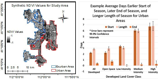
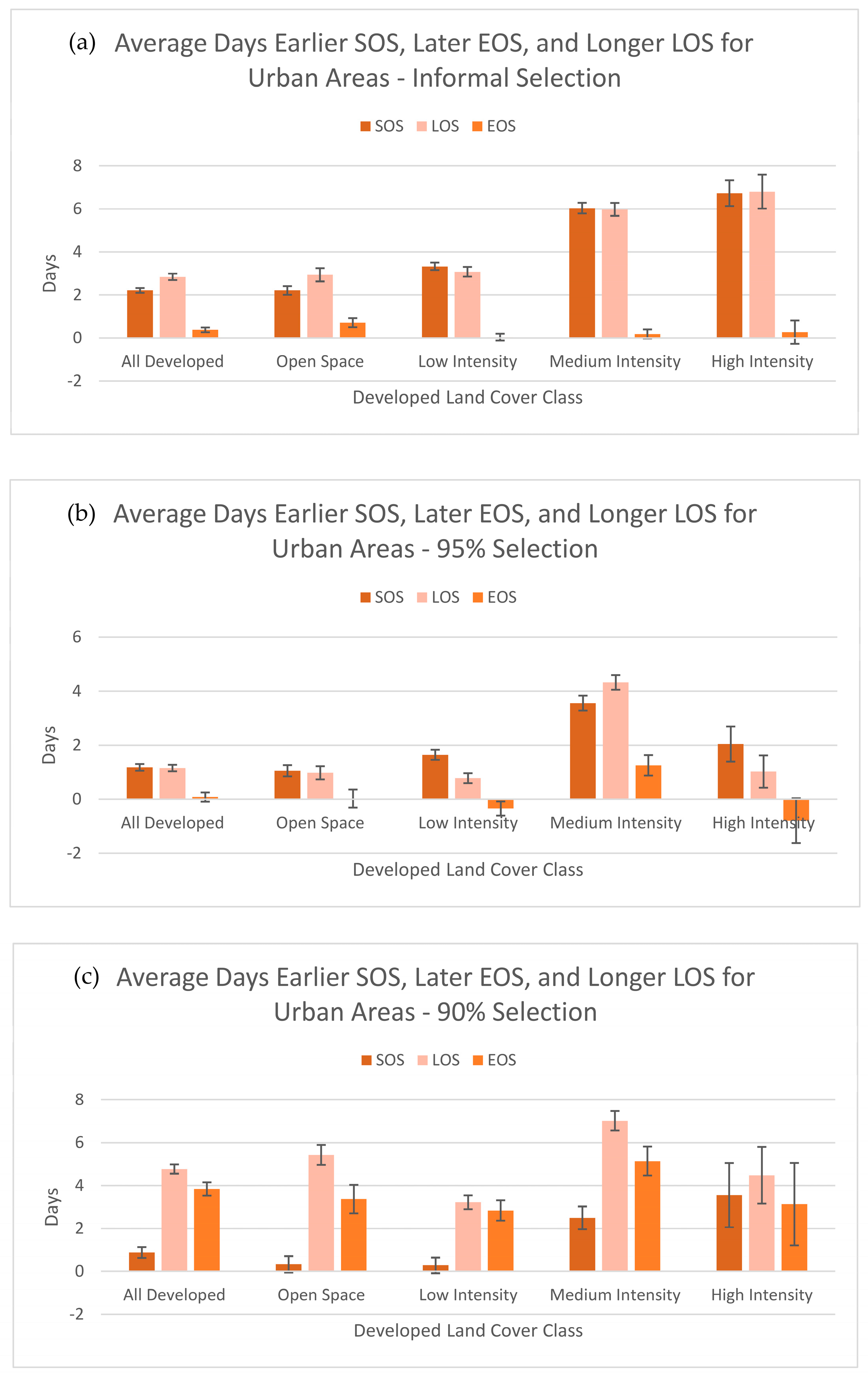
The normalized data of the informal selection show an earlier SOS for urban areas by a factor of 2.21 to 6.73 days on average, depending on the class. The more developed classes had the biggest difference in SOS and the least developed classes along with all of the classes together had the smallest difference. Although the developed areas as a whole and individual classes both show a later EOS for the urban areas, the number of days between the mean EOS for the urban and the exurban area had a lower range that was from 0.04 to 0.71 days. Lastly, the difference in the average length of season was longer in urban areas and ranges from being 2.84 days for all developed areas up to 6.8 days longer for the most developed areas, with the difference increasing for each class with percent imperviousness (Figure 6a). Standard deviations for the years were generally largest for the LOS parameter (

Table 4. Standard deviations for the normalized data.

		All Developed	Open Space	Low Intensity	Medium Intensity	High Intensity
Informal Base Pair Selection	SOS Urban	18.4	16.6	16.3	17.7	21.7
	SOS Exurban	17.7	16.0	16.4	17.6	22.9
	EOS Urban	17.6	17.9	16.1	16.5	22.0
	EOS Exurban	19.7	19.3	18.6	20.2	25.3
	LOS Urban	24.5	24.9	22.3	23.3	29.9
	LOS Exurban	26.2	25.8	24.5	25.9	35.1
95% Clear Base Pair Selection	SOS Urban	19.0	16.4	16.8	18.6	26.0
	SOS Exurban	19.2	17.5	18.4	19.8	22.3
	EOS Urban	19.1	20.1	17.6	17.9	23.7
	EOS Exurban	21.7	21.7	20.8	22.4	24.1
	LOS Urban	26.1	25.7	23.7	25.2	34.0
	LOS Exurban	29.4	29.5	28.5	29.9	31.9
90% Clear Base Pair Selection	SOS Urban	28.3	22.7	27.3	28.8	35.5
	SOS Exurban	24.6	22.0	24.3	26.1	29.4
	EOS Urban	24.4	26.3	23.8	22.9	30.4
	EOS Exurban	27.3	27.3	26.3	28.4	31.9
	LOS Urban	36.8	36.6	35.9	36.5	47.3
	LOS Exurban	36.9	36.5	35.8	38.6	42.8

).

The normalized data of the 95% statistical selection threshold show an earlier SOS for urban areas by a factor of 1.05 to 3.56 days on average. Although the developed areas as a whole and the two classes of developed open space and developed medium intensity show a later EOS for the urban areas up to 1.25 days, the other two classes show a later EOS for the exurban area of 0.35 and 0.79 days. Again, the difference in the average length of season was longer in urban areas and ranges from being 0.78 days up to 4.32 days longer. The difference for each class does not consistently increase with percent imperviousness (Figure 6b).

The normalized data of the 90% statistical selection threshold on STARFM version 1.2.1 also show an earlier SOS for all urban areas ranging from 0.28 to 3.55 days. All developed areas as a whole and all four classes show a later EOS for the urban areas ranging from 2.84 to 5.15 days. Again, the difference in the average length of season was longer in urban areas and ranges from being 3.22 and 7.02 days longer (Figure 6c).

To see how consistent these overall findings were from year to year between classes, one can also look at the 11 years separately. This showed that the average urban SOS date was earlier for up to all of the 11 years for developed high intensity urban areas when using informal base pair selection criteria, but also earlier in only six years when using 90% selection criteria for developed low intensity areas. The average EOS date was later for the urban areas from as few as three out of the 11 years to as many as nine, with all three selection methods showing the least amount of years in the developed high intensity class. The average LOS was longer in the urban areas for 10 out of 10 years for developed open space with an informal selection and for only six years for various classes with both the 90% and 95% selection criteria (

Table 5. Frequencies of years where mean SOS was earlier, EOS was later, and LOS was longer in the urban areas according to base pair selection.

Years with Earlier Urban SOS	Informal Selection	95% Selection	90% Selection
All Developed Areas	9	8	7
Developed Open Space	9	8	8
Developed Low Intensity	8	8	6
Developed Medium Intensity	10	7	7
Developed High Intensity	11	8	8
Years with Later Urban EOS
All Developed Areas	7	6	8
Developed Open Space	9	7	8
Developed Low Intensity	6	7	8
Developed Medium Intensity	7	8	9
Developed High Intensity	3	3	6
Years with longer Urban LOS
All Developed Areas	7	7	6
Developed Open Space	10	6	8
Developed Low Intensity	9	6	6
Developed Medium Intensity	8	7	7
Developed High Intensity	8	6	6

).

3.3. Tests for Variance Equality and Normality

Based on the results of the F-tests, almost all land cover classes and the developed areas as a whole had statistically unequal variances between the urban and exurban areas. The exceptions to this were the informal selection developed medium intensity land cover class for the SOS and the 90% selection criteria’s LOS for all developed areas, developed open space and developed low intensity, where all p-value were above 0.1. Visual inspection of all histograms showed an approximate normal distribution (see Supplementary Materials for the histograms). This method was chosen over a statistical test due to small deviations from normality being marked as significant even though they should not affect parametric test results [53].

3.4. Tests for Inequality of Phenological Parameters

RStudio performed a two-tailed and two-sample t-test for each parameter and each developed area as a whole as well as each land cover class separately to see if the mean of the urban area was statistically different from the mean of the exurban area. The t-test assumed unequal variances in all cases except when the F-test could not show an unequal variance. The tests showed that for the SOS, both the informal and 95% selection criteria show a statistical difference between the urban and exurban areas at the 99.9% level for all areas together and all classes separately, with all observed p-values of <2.2 × 10⁻¹⁶. However, after applying a Bonferroni correction, the 90% selection criteria only shows a 99.9% significant difference for all developed areas, developed medium intensity, and developed high intensity areas, with p-values of <2.2 × 10⁻¹⁶ for all developed areas and medium developed areas and 4.91 × 10⁻¹⁵ for developed high intensity areas. It also shows an insignificant difference in the SOS for both developed open space and developed low intensity with p-values of 0.0045 and 0.013, respectively.

The EOS results were all statistically significant at the 99.9% level, with all observed p-values of <2.2 × 10⁻¹⁶, for the 90% selection criteria. However, they were mixed for both the informal and 95% selection criteria. With the informal selection criteria, both developed areas as a whole and developed open space had an observed p-value of <2.2 × 10⁻¹⁶. After applying a Bonferroni correction for the remaining classes, the results show no statistical difference for EOS in the developed low intensity, developed medium intensity, and developed high intensity classes with observed p-values of 0.448, 0.011, and 0.107, respectively. With the 95% selection criteria, both developed low intensity and medium intensity were statistically significant with p-values of 6.5 × 10⁻¹⁰ and <2.2 × 10⁻¹⁶, respectively, and after the Bonferroni correction developed high intensity was significant at the 99% level with an observed p-value of 0.000012. There was no significance for the remaining classes after a Bonferroni correction with all developed areas having a p-value of 0.03 and developed open space having a p-value of 0.75.

The length of season showed the most consistent results with most classes for all methods having an observed p-value of <2.2 × 10⁻¹⁶ making them significant at the 99.9% level. The only exceptions to this were the developed high intensity results for both the 95% and 90% selection methods. The 90% selection criteria results were still significant at the 99.9% level but the observed p-value was 1.5 × 10⁻¹⁴. The 95% selection method still did show significance at the 99% level after a Bonferroni correction with an observed p-value of 0.000049.

4. Discussion

4.1. Start of Season

Our study analyzed the effects of UHI on phenology in urban areas, although we did not attempt to measure temperature for each land cover per se. Instead, we used percent imperviousness to understand the spatial variability of temperature in cities. Since UHI is the direct product of the transformation of natural landscapes into an impervious man-made urban texture [3] and a strong linear relationship between the percent impervious surface area and land surface temperature has been shown [54], it is reasonable to assume that the areas we defined as urban are warmer than the areas we defined as exurban. Based on previous findings suggesting that leaves appear earlier during a warmer spring [11] and that leaves develop earlier in cities [6], we reasonably expected our urbanized areas to exhibit an earlier SOS, which was supported by the results of this study, although not statistically when using STARFM v1.2.1 and a 90% selection criteria for all classes. Therefore, base pair selection and software version may make a difference when observing SOS of the urban environment. In addition, it has been shown that temporal gradients in leaf onset varies [55], which coincides with our findings of a large standard deviation for SOS (Table 4).

Interestingly, our results do not show a similar magnitude of differences in the SOS between classes throughout the urban and exurban area. This coincides with the case study by Melaas et al. [56], which showed that the amount of impervious surface area in surrounding vegetation patches influences the timing of SOS. Although we do not show a clear trend with the difference in SOS growing as mean percent imperviousness does, for all three selection methods the difference in mean days becomes larger between urban and exurban areas for the two most developed classes when compared to the two least developed classes. In addition, out of all 11 years where SOS was calculated, all methods showed an earlier urban SOS for all classes more times than a later urban SOS. However, there is a range to the number of years where urban SOS is earlier. Based on this, there is not a uniform effect on the SOS throughout the entire urban area. In addition, it is reasonable to assume that we may lose some information if we generalize entire municipalities as having an earlier SOS. For this reason, having a spatial resolution finer than that of MODIS, such as that produced by fused data, would allow for a better understanding of the complex relationships between heterogeneous urban and exurban environments.

4.2. End of Season

The EOS results were not as conclusive as the SOS results, which is not surprising since previous research also found an unclear association between the urban-exurban differences and autumn phenophases [6] and high variability in the difference [57]. Even though the mean EOS was later for urban areas in 13 out of 15 of the stacked datasets, the statistical significance across all classes was present only when the 90% criteria was used. This also indicates that base pair and software selection may lead to different results than when looking at features or specific locations within the municipality. This supports previous findings that EOS in urban vegetation patches is influenced by the percent impervious surface of surrounding patches [56].

There are two potential reasons for such findings of EOS inconsistency between base pair selection and software. First, there could be a consistent and large difference in the EOS, as the 90% selection criteria with STARFM v 1.2.1 showed, but our methods were too simplistic or introduced excessive errors so the difference was improperly observed with using an informal and 95% selection criteria and STARFM v1.1.2. Second, there are potentially other environmental factors that are similar between the urban and exurban area, which are the main cues for trees to start growth cessation. For example, Perry [12] points to the shortening of the photoperiod. If this were true, we would not expect the UHI to change EOS. In addition, this would mean that the difference in EOS shown when using the 90% criteria is a result of observing a sample of the EOS under control of another environmental factor such as, for example, photoperiod.

4.3. Length of Season

Although LOS is the only phenological parameter that is consistently statistically significant, we are cautious of these results. Both the SOS and EOS contribute to the LOS, and under an informal and 95% selection criteria the most reliable contributor to the statistically longer growing season in the urban area is the earlier start in the spring. As shown in Figure 6a,b, the difference in the SOS for the urban and exurban area is proportionally larger than the EOS, thus contributing more to the difference in the LOS. In addition, even without statistically different EOS dates for all of the classes with these two methods, the difference in the LOS is still statistically significant for all classes. However, when we look at LOS derived from the 90% criteria, the opposite is true that without all statistically different SOS dates, the difference in the LOS is still statistically significant for all classes. Therefore, since there is uncertainty with why LOS is longer in the urban areas, it is difficult to support that it is true.

Moreover, when looking at the mean LOS for each class, a similar trend appears as we see with the SOS, which is that there is a difference in the LOS across classes. Once again, this observation suggests to look at intra-city features and not just the urban area as a whole to be able to describe better the effects of the urban environment on phenology.

4.4. Study Assumptions and Potential Limitations

The method we used for normalization ensures that all data obtained are used. It also corrects for interannual shifts in phenological parameters by placing the event at each location in relation to the expected date of the same exurban event for the same year. This allows for the comparison of the difference in time between an event at each location and the timing of the corresponding expected exurban area’s event and not a comparison of the actual dates, which may not be comparable from one year to the next due to changing weather patterns. Thus, after normalization, one can compare the urban and exurban data to show the differences within each separate year and also among all years together. Importantly, the approach accounts for the uneven and inconsistent sample proportions between the urban and exurban environments from year to year. Simply normalizing according to the mean value of all urban and exurban pixels would pull the normalized value in different amounts, based on the proportional size, toward the sample with the larger size and not centering the normalized values at the same value from year to year. For example, if one year had one exurban point for every two urban points and the next year this ratio decreased to 1:4, the normalized values of the second year would be pulled closer to zero for the urban areas and further from zero for the exurban areas, making them incomparable.

However, an underlying assumption of this normalization method is that if a shift in dates does occur from one year to the next, the amount of the shift is the same for both the urban and exurban environment. If this assumption is violated, any disproportional interannual shifts would skew the results to either be over or under represented depending on if the urban sample size was large or small for that year.

A second underlying assumption of this study is that the expected vegetation type and management practices were similar between like land cover classes for both the urban and rural environments. For example, it was assumed that any influences a homeowner may have on phenology due to landscaping practices (i.e., watering the lawn in the spring) and vegetation transplanting (i.e., planting grass for a lawn) were just as likely to occur regardless if the individual lives in a rural and urban settings. This is an important assumption, as it has been observed that phenological traits can differ between vegetation types [51]. However, making comparisons between the urban and rural environments of developed areas with the same land cover classes controlled for this, as opposed to comparing dissimilar land cover classes that may have dissimilar landscape management techniques.

The third assumption is that changes in NVDI values accurately represent changes in phenological parameters. The current study used changes in NDVI as a proxy for growing season parameters. However, it is not well understood how well these values, derived from fused imagery, correspond to the actual ground events of SOS, EOS, and LOS. The Collection 5 MODIS NBAR data used in this study were the 8-day overlapping product that is collected over 16 days. Depending on the data availability during the 16-day period especially around the SOS and EOS dates, we could miss or smooth the small changes from the multi-date data products.

The fourth limitation is that we did not attempt to resolve any potential errors with the NLCD classifications. Although overall accuracies were 79% and 78% for the previous Level II NLCD versions from 2001 and 2006, respectively, they did have difficulty distinguishing the context of grass. In relation to the land cover classes we looked at, the 2006 NLCD had a producer’s accuracy of 42%, 70%, 80%, and 26% for classes 21, 22, 23, and 24, respectively. The user’s accuracies for these classes were 52%, 59%, 69%, and 83%, respectively. The 2001 NLCD accuracy was similar (within 5%) to the 2006 accuracies except for the producer’s accuracy for class 24, which was 81% [58].

The last assumption is that our sample was representative of the conditions of the entire urban and exurban areas. We had a very large sample, so this is reasonable to assume. However, the areas of no data predictions could be biased due to some uniform trait and therefor underrepresented. For example, the proportion of the sample remaining toward the center of the urban and exurban areas was similar for the informal and 95% selection criteria. However, for the 90% selection criteria the central areas were disproportionally under represented (

Table 6. Total original sample size for all developed areas based on base pair selection and the percent of the original sample remaining 500 m and 1500 m inward away from the urban and exurban edges.

	Parameter	Total Sample Size	Percent Remaining at 500 m Inward	Percent Remaining at 1500 m Inward
Informal Selection	SOS	1,241,726	56	12
	EOS	1,681,156	56	13
>95% Selection	SOS	1,263,499	56	13
	EOS	1,632,057	57	13
>90% Selection	SOS	511,615	45	5
	EOS	634,573	44	5

). Previous research [21] has shown a relationship between the UHI and distance to urban core area and should be considered.

In addition, selecting Landsat images with less than 10% cloud cover as an initial screening process could potentially omit additional dates of clear Landsat images for the study area, thus reducing the number of base pairs used. Based on previous research [59], the risk of omitting these scenes potentially leads to a less than optimal quality of fused image since there could have been a potential base date nearer to some of our predicted dates than what we used for prediction. Adding to this, using a visual inspection to remove Landsat images could introduce human error.

4.5. Future Work

Future research should attempt to identify the source of variation that caused inconsistent results, being cautious of how input data would affect their sample distribution and validity of predictions. Evaluating base pair selection should include not only ensuring a valid fused image, but also taking into account how the distribution will affect the location of no data and how this in turn affects TIMESAT. Since the difference in base pair selection method does not produce large differences in the validity of our fused images, how the data and parameters can affect the ability of TIMESAT to make predictions is important to consider.

The MODIS collection 6 now provides daily NBAR product at 500 m resolution which could be utilized in data fusion. The BRDF corrected daily surface reflectance is another option to use in the future. The daily MODIS products may be able to reduce uncertainties in extracting phenological parameters. This study used Landsat 5 TM data for data consistency. Landsat 7 ETM+ data even with the Scan-Line-Corrector errors can still be used to increase the frequency of high resolution data. Other recent high resolution data such as Landsat 8 and Sentinel-2 can be included in the future. The Landsat and MODIS pair images may be gap-filled first before data fusion to increase valid prediction. Different weights from original and the fused data sources may be considered similar to the strategy used in mapping crop phenology [30].

The results of future work should also validate the predicted phenological dates derived from STARFM synthetic imagery against in situ observations of phenological parameters for the urban and exurban environments, preferably for a variety of land cover classes. In addition, our study was confined to a very specific environment and may not be generalizable to a variety of areas. Expanding the prediction to a variety of climates and cities would help to overcome this. Last, the value of using a fusion model over one source of satellite data to predict the differences in the urban and exurban growing seasons should be explored. Our next steps will be to attempt to model LSP parameters with high resolution/low frequency and low resolution/high frequency data alone. This will allow making conclusions about the amount of information gained from fusing the data in regards to observing the effects of the UHI on phenology.

Beyond lacking in comparisons to other data sources and locations, the current study did not aim to explore in depth how different land cover classes affect phenological events. Although this paper described the difference in mean urban and exurban values among land cover classes, it was limited to a simple descriptive analysis. In addition, it may be interesting to see if there is a shift in calendar dates of phenological events for both urban and exurban environments, rather than just look at the shift in the number of days of the normalized difference between the two as we did.

5. Conclusions

This study has uncertainties, but it offers encouragement that STARFM can be sensitive enough to detect the change in phenological parameters of vegetation that we would expect to see because of the UHI effect in urbanized landscapes. Although base pair selection for image fusion did not strongly affect the validity of fused images, it did have a noticeable effect on the phenology results. We suspect that this is in part due to the changing distribution of where no data are available for TIMESAT to fit. As the number of base pairs increases, so will the potential locations of no data from Landsat that is masked out from a prediction. As we saw with disproportional distribution of no data in one instance, these no data points might not be randomly distributed and therefore skew any results. We believe that this could have skewed the results for the 90% base pair selection because we not only added in the potential for an additional 5% unclear pixel coverage, but also due to the software change. STARFM v1.2.1 added in a strict validation that may potentially not allow a prediction to be made in areas where it did before, thus compromising a lesser sample size for an increase in overall prediction quality and not covering up any bias distribution in no data.

Our statistical results are mixed, but generally, they support the notion that the UHI leads to an early start of growing season (SOS) and an overall increase in the length of the growing season (LOS). Conversely, the results show that depending on the methods used to select base pairs and the software version used to make the predictions, the effects urban areas have on the timing of the end of the growing season (EOS) can fluctuate. By using the fusion method, we were able to work toward understanding some of the advantages and challenges of modeling the heterogeneous urban landscape while preserving temporal accuracy. Overall, it allowed us to not only see a difference in phenological parameters between urban and exurban areas, but also to see that regardless of fusion method, there is variability among phenological parameters according to the land cover class at 30 m resolution. Depending on the base pair selection and version of STARFM, the differences in mean earlier urban SOS between land cover classes within each selection criteria ranged from as many as 4.5 to as few as 2.5 days, the differences in mean EOS urban delay between land cover classes ranged from 0.67 to 2.3 days, and the differences in mean longer urban LOS ranged from 3.6 to 3.9 days. Without having the temporal and spatial resolution of a fused image, these intercity variations in phenological parameters might not be observable.

However, how well the changes detected correlate to actual in situ conditions and the actual timing of phenological events is unknown. Lastly, it has yet to be determined how much information that describes phenology is gained by fusing the data and to what extent errors are introduced into these estimations.

References

1. United Nations. United Nations World Urbanization Prospects; the 2014 Revision; United Nations: New York, NY, USA, 2014. [Google Scholar]
2. Oke, T.R. The energetic basis of the urban heat island. Q. J. R. Meteorol. Soc. 1982, 108, 1–24. [Google Scholar] [CrossRef]
3. Luo, Z.; Asproudi, C. Subsurface urban heat island and its effects on horizontal ground-source heat pump potential under climate change. Appl. Therm. Eng. 2015, 90, 530–537. [Google Scholar] [CrossRef]
4. Hartmann, D.L.; Klein Tank, A.M.G.; Rusticucci, M.; Alexander, L.V.; Brönnimann, S.; Charabi, Y.; Dentener, F.J.; Dlugokencky, E.J.; Easterling, D.R.; Kaplan, A.; et al. Observations: Atmosphere and Surface. In Climate Change 2013: The Physical Science Basis. Contribution of Working Group I to the Fifth Assessment Report of the Intergovernmental Panel on Climate Change; Stocker, T.F., Qin, D., Plattner, G.-K., Tignor, M., Allen, S.K., Boschung, J., Nauels, A., Xia, Y., Bex, V., Midgley, P.M., Eds.; Cambridge University Press: Cambridge, UK; New York, NY, USA, 2013; pp. 159–254. [Google Scholar]
5. Tan, M.; Li, X. Quantifying the effects of settlement size on urban heat islands in fairly uniform geographic areas. Habitat Int. 2015, 49, 100–106. [Google Scholar] [CrossRef]
6. Jochner, S.; Menzel, A. Urban phenological studies—Past, present, future. Environ. Pollut. 2015, 203, 250–261. [Google Scholar] [CrossRef] [PubMed]
7. Ziska, L.H.; Gebhard, D.E.; Frenz, D.A.; Faulkner, S.; Singer, B.D.; Straka, J.G. Cities as harbingers of climate change: Common ragweed, urbanization, and public health. J. Allergy Clin. Immunol. 2003, 111, 290–295. [Google Scholar] [CrossRef] [PubMed]
8. Walker, J.J.; de Beurs, K.M.; Henebry, G.M. Land surface phenology along urban to rural gradients in the U.S. Great Plains. Remote Sens. Environ. 2015, 165, 42–52. [Google Scholar] [CrossRef]
9. Badeck, F.-W.; Bondeau, A.; Böttcher, K.; Doktor, D.; Lucht, W.; Schaber, J.; Sitch, S. Responses of spring phenology to climate change. New Phytol. 2004, 162, 295–309. [Google Scholar] [CrossRef]
10. Häkkinen, R.; Linkosalo, T.; Hari, P. Effects of dormancy and environmental factors on timing of bud burst in Betula pendula. Tree Physiol. 1998, 18, 707–712. [Google Scholar] [CrossRef] [PubMed]
11. Wesołowski, T.; Rowiński, P. Timing of bud burst and tree-leaf development in a multispecies temperate forest. For. Ecol. Manag. 2006, 237, 387–393. [Google Scholar] [CrossRef]
12. Perry, T.O. Dormancy of trees in winter. Science 1971, 171, 29–36. [Google Scholar] [CrossRef] [PubMed]
13. Heide, O.M. Growth and dormancy in Norway Spruce Ecotypes (Picea abies) I. Interaction of photoperiod and temperature. Physiol. Plant. 1974, 30, 1–12. [Google Scholar] [CrossRef]
14. Peñuelas, J.; Rutishauser, T.; Filella, I. Phenology feedbacks on climate change. Science 2009, 324, 887–888. [Google Scholar] [CrossRef] [PubMed]
15. Richardson, A.D.; Keenan, T.F.; Migliavacca, M.; Ryu, Y.; Sonnentag, O.; Toomey, M. Climate change, phenology, and phenological control of vegetation feedbacks to the climate system. Agric. For. Meteorol. 2013, 169, 156–173. [Google Scholar] [CrossRef]
16. Schwartz, M.D.; Karl, T.R. Spring phenology: Nature’s experiment to detect the effect of “green-up” on surface maximum temperatures. Mon. Weather Rev. 1990, 118, 883–890. [Google Scholar] [CrossRef]
17. Peñuelas, J.; Filella, I. Responses to a warming world. Science 2001, 294, 793–795. [Google Scholar] [CrossRef] [PubMed]
18. Richardson, A.D.; Hollinger, D.Y.; Dail, D.B.; Lee, J.T.; Munger, J.W.; O’keefe, J. Influence of spring phenology on seasonal and annual carbon balance in two contrasting New England forests. Tree Physiol. 2009, 29, 321–331. [Google Scholar] [CrossRef] [PubMed]
19. Primack, R.B.; Ibáñez, I.; Higuchi, H.; Lee, S.D.; Miller-Rushing, A.J.; Wilson, A.M.; Silander, J.A., Jr. Spatial and interspecific variability in phenological responses to warming temperatures. Biol. Conserv. 2009, 142, 2569–2577. [Google Scholar] [CrossRef]
20. De Beurs, K.M.; Henebry, G.M. Land surface phenology, climatic variation, and institutional change: Analyzing agricultural land cover change in Kazakhstan. Remote Sens. Environ. 2004, 89, 497–509. [Google Scholar] [CrossRef]
21. Zhang, X.; Friedl, M.A.; Schaaf, C.B.; Strahler, A.H.; Schneider, A. The footprint of urban climates on vegetation phenology. Geophys. Res. Lett. 2004, 31, L12209. [Google Scholar] [CrossRef]
22. Holben, B.N. Characteristics of maximum-value composite images from temporal AVHRR data. Int. J. Remote Sens. 1986, 7, 1417–1434. [Google Scholar] [CrossRef]
23. Liang, S.; Fang, H.; Chen, M. Atmospheric correction of Landsat ETM+ land surface imagery—Part I: Methods. IEEE Trans. Geosci. Remote Sens. 2001, 39, 2490–2498. [Google Scholar] [CrossRef]
24. Van de Voorde, T.; Jacquet, W.; Canters, F. Mapping form and function in urban areas: An approach based on urban metrics and continuous impervious surface data. Landsc. Urban Plan. 2011, 102, 143–155. [Google Scholar] [CrossRef]
25. Zhang, X.; Friedl, M.A.; Schaaf, C.B. Sensitivity of vegetation phenology detection to the temporal resolution of satellite data. Int. J. Remote Sens. 2009, 30, 2061–2074. [Google Scholar] [CrossRef]
26. Pohl, C.; Van Genderen, J.L. Multisensor image fusion in remote sensing: Concepts, methods and applications. Int. J. Remote Sens. 1998, 19, 823–854. [Google Scholar] [CrossRef]
27. Emelyanova, I.V.; McVicar, T.R.; Van Niel, T.G.; Li, L.T.; van Dijk, A.I.J.M. Assessing the accuracy of blending Landsat-MODIS surface reflectances in two landscapes with contrasting spatial and temporal dynamics: A framework for algorithm selection. Remote Sens. Environ. 2013, 133, 193–209. [Google Scholar] [CrossRef]
28. Gao, F.; Masek, J.; Schwaller, M.; Hall, F. On the blending of the Landsat and MODIS surface reflectance: Predicting daily Landsat surface reflectance. IEEE Trans. Geosci. Remote Sens. 2006, 44, 2207–2218. [Google Scholar]
29. Liang, L.; Schwartz, M.D.; Wang, Z.; Gao, F.; Schaaf, C.B.; Tan, B.; Morisette, J.T.; Zhang, X. A Cross Comparison of spatiotemporally enhanced springtime phenological measurements from satellites and ground in a Northern U.S. mixed forest. IEEE Trans. Geosci. Remote Sens. 2014, 52, 7513–7526. [Google Scholar] [CrossRef]
30. Gao, F.; Anderson, M.C.; Zhang, X.; Yang, Z.; Alfieri, J.G.; Kustas, W.P.; Mueller, R.; Johnson, D.M.; Prueger, J.H. Toward mapping crop progress at field scales through fusion of Landsat and MODIS imagery. Remote Sens. Environ. 2017, 188, 9–25. [Google Scholar] [CrossRef]
31. Shen, H.; Huang, L.; Zhang, L.; Wu, P.; Zeng, C. Long-term and fine-scale satellite monitoring of the urban heat island effect by the fusion of multi-temporal and multi-sensor remote sensed data: A 26-year case study of the city of Wuhan in China. Remote Sens. Environ. 2016, 172, 109–125. [Google Scholar] [CrossRef]
32. Olexa, E.M.; Lawrence, R.L. Performance and effects of land cover type on synthetic surface reflectance data and NDVI estimates for assessment and monitoring of semi-arid rangeland. Int. J. Appl. Earth Obs. Geoinf. 2014, 30, 30–41. [Google Scholar] [CrossRef]
33. National Land Cover Database 2011 (NLCD2011). Available online: https://www.mrlc.gov/nlcd11_data.php (accessed on 19 January 2017).
34. Imhoff, M.L.; Zhang, P.; Wolfe, R.E.; Bounoua, L. Remote sensing of the urban heat island effect across biomes in the continental USA. Remote Sens. Environ. 2010, 114, 504–513. [Google Scholar] [CrossRef]
35. Artis, D.A.; Carnahan, W.H. Survey of emissivity variability in thermography of urban areas. Remote Sens. Environ. 1982, 12, 313–329. [Google Scholar] [CrossRef]
36. Sobrino, J.A.; Jiménez-Muñoz, J.C.; Paolini, L. Land surface temperature retrieval from LANDSAT TM 5. Remote Sens. Environ. 2004, 90, 434–440. [Google Scholar] [CrossRef]
37. USGS. Query Form for the United States and Its Territories. Available online: http://geonames.usgs.gov/apex/f?p=gnispq (accessed on 29 August 2016).
38. NOAA. Salt Lake City Climate Book. Available online: http://www.wrh.noaa.gov/slc/climate/slcclimate/SLC/index.php (accessed on 29 August 2016).
39. Walker, J.J.; de Beurs, K.M.; Wynne, R.H.; Gao, F. Evaluation of Landsat and MODIS data fusion products for analysis of dryland forest phenology. Remote Sens. Environ. 2012, 117, 381–393. [Google Scholar] [CrossRef]
40. United States Geological Survey (USGS). USGS Product Guide: Landsat 4-7 Climate Data record (CDR) Surface Reflectance; version 6.0; United States Geological Survey: Sioux Falls, SD, USA, 2015.
41. ArcGIS Desktop, Release 10; Environmental Systems Research Institute: Redlands, CA, USA, 2010.
42. Martonchik, J.V.; Bruegge, C.J.; Strahler, A.H. A review of reflectance nomenclature used in remote sensing. Remote Sens. Rev. 2000, 19, 9–20. [Google Scholar] [CrossRef]
43. Masek, J.G.; Vermote, E.F.; Saleous, N.E.; Wolfe, R.; Hall, F.G.; Huemmrich, K.F.; Gao, F.; Kutler, J.; Lim, T.-K. A Landsat surface reflectance dataset for North America, 1990–2000. IEEE Geosci. Remote Sens. Lett. 2006, 3, 68–72. [Google Scholar] [CrossRef]
44. NASA. MODIS/Terra Data Outages. Available online: http://modaps.nascom.nasa.gov/services/production/outages_terra.html (accessed on 29 August 2016).
45. Tucker, C.J. Red and photographic infrared linear combinations for monitoring vegetation. Remote Sens. Environ. 1979, 8, 127–150. [Google Scholar] [CrossRef]
46. Myneni, R.B.; Hall, F.G.; Sellers, P.J.; Marshak, A.L. The interpretation of spectral vegetation indexes. IEEE Trans. Geosci. Remote Sens. 1995, 33, 481–486. [Google Scholar] [CrossRef]
47. Marchetti, Z.Y.; Minotti, P.G.; Ramonell, C.G.; Schivo, F.; Kandus, P. NDVI patterns as indicator of morphodynamic activity in the middle Paraná River floodplain. Geomorphology 2016, 253, 146–158. [Google Scholar] [CrossRef]
48. Jönsson, P.; Eklundh, L. Seasonality extraction by function fitting to time-series of satellite sensor data. IEEE Trans. Geosci. Remote Sens. 2002, 40, 1824–1832. [Google Scholar] [CrossRef]
49. Jönsson, P.; Eklundh, L. TIMESAT—A program for analyzing time-series of satellite sensor data. Comput. Geosci. 2004, 30, 833–845. [Google Scholar] [CrossRef]
50. Eklundh, L.; Jönsson, P. TIMESAT 3.2 with Parallel Processing Software Manual; Lund University: Lund, Sweden, 2015. [Google Scholar]
51. Zipper, S.C.; Schatz, J.; Singh, A.; Kucharik, C.J.; Townsend, P.A.; Loheide II, S.P. Urban heat island impacts on plant phenology: Intra-urban variability and response to land cover. Environ. Res. Lett. 2016, 11, 054023. [Google Scholar] [CrossRef]
52. RStudio Team. RStudio: Integrated Development for R; RStudio, Inc.: Boston, MA, USA, 2015. [Google Scholar]
53. Öztuna, D.; Elhan, A.H.; Tüccar, E. Investigation of Four different normality tests in terms of type 1 error rate and power under different distributions. Turk. J. Med. Sci. 2006, 36, 171–176. [Google Scholar]
54. Yuan, F.; Bauer, M.E. Comparison of impervious surface area and normalized difference vegetation index as indicators of surface urban heat island effects in Landsat imagery. Remote Sens. Environ. 2007, 106, 375–386. [Google Scholar] [CrossRef]
55. Fisher, J.I.; Mustard, J.F.; Vadeboncoeur, M.A. Green leaf phenology at Landsat resolution: Scaling from the field to the satellite. Remote Sens. Environ. 2006, 100, 265–279. [Google Scholar] [CrossRef]
56. Melaas, E.K.; Wang, J.A.; Miller, D.L.; Friedl, M.A. Interactions between urban vegetation and surface urban heat islands: A case study in the Boston metropolitan region. Environ. Res. Lett. 2016, 11, 054020. [Google Scholar] [CrossRef]
57. White, M.A.; Nemani, R.R.; Thornton, P.E.; Running, S.W. Satellite evidence of phenological differences between urbanized and rural areas of the Eastern United States deciduous broadleaf forest. Ecosystems 2002, 5, 260–273. [Google Scholar] [CrossRef]
58. Wickham, J.D.; Stehman, S.V.; Gass, L.; Dewitz, J.; Fry, J.A.; Wade, T.G. Accuracy assessment of NLCD 2006 land cover and impervious surface. Remote Sens. Environ. 2013, 130, 294–304. [Google Scholar] [CrossRef]
59. Fu, D.; Zhang, L.; Chen, H.; Wang, J.; Sun, X.; Wu, T. Assessing the effect of temporal interval length on the blending of Landsat-MODIS surface reflectance for different land cover types in Southwestern Continental United States. ISPRS Int. J. GeoInf. 2015, 4, 2542–2560. [Google Scholar] [CrossRef]
Figure 1. Location map of the study area within the contiguous United States and mean impervious surface and urban/exurban classification by municipality.
Remotesensing 09 00099 g001
Figure 2. The steps contained in the python script to process the MODIS and Landsat data for input into STARFM.
Remotesensing 09 00099 g002
Figure 3. The temporal distribution of the Landsat scenes used in the base pairing.
Remotesensing 09 00099 g003
Figure 4. The steps contained in the python script to match MODIS scenes without a corresponding Landsat scene with the appropriate MODIS/Landsat base pair and create the STARFM input texts reflecting this.
Remotesensing 09 00099 g004
Figure 5. Example synthetic NDVI image.
Remotesensing 09 00099 g005
Figure 6. Three bar charts showing the approximate average number of days the SOS is earlier, EOS is later, and LOS is longer in the urban area for (a) the informal selection criteria, (b) the 95% statistical criteria, and (c) the 90% statistical selection criteria. Error bars represent a 99.9% confidence interval.
Remotesensing 09 00099 g006