3D Monitoring of Buildings Using TerraSAR-X InSAR, DInSAR and PolSAR Capacities

1
School of Geosciences, The University of Edinburgh, Edinburgh EH8 9XP, UK
2
The French Aerospace Lab, ONERA, 91120 Palaiseau, France
3
Telecom ParisTech, 75013 Paris, France
*
Author to whom correspondence should be addressed.
Remote Sens. 2017, 9(10), 1010; https://doi.org/10.3390/rs9101010
Submission received: 30 June 2017
/
Revised: 21 August 2017
/
Accepted: 22 September 2017
/
Published: 29 September 2017
(This article belongs to the Special Issue Recent Advances in Polarimetric SAR Interferometry)
Abstract
:The rapid expansion of cities increases the need of urban remote sensing for a large scale monitoring. This paper provides greater understanding of how TerraSAR-X (TSX) high-resolution abilities enable to reach the spatial precision required to monitor individual buildings, through the use of a 4 year temporal stack of 100 images over Paris (France). Three different SAR modes are investigated for this purpose. First a method involving a whole time-series is proposed to measure realistic heights of buildings. Then, we show that the small wavelength of TSX makes the interferometric products very sensitive to the ordinary building-deformation, and that daily deformation can be measured over the entire building with a centimetric accuracy, and without any a priori on the deformation evolution, even when neglecting the impact of the atmosphere. Deformations up to 4 cm were estimated for the Eiffel Tower and up to 1 cm for other lower buildings. These deformations were analyzed and validated with weather and in situ local data. Finally, four TSX polarimetric images were used to investigate geometric and dielectric properties of buildings under the deterministic framework. Despite of the resolution loss of this mode, the possibility to estimate the structural elements of a building orientations and their relative complexity in the spatial organization are demonstrated.
1. Introduction
Cities play a major role in society. They are rather complex and evolve rapidly, therefore they need dedicated reliable monitoring techniques. For example, it can be needed for urban managers to update a land-use map to plan infrastructures improvement or make a diagnosis after natural disaster to help rescuers or plan the rebuild of the city. Remote sensing, and more specifically radar images might successfully address these needs. Hence, radar imaging is a reference tool for the monitoring of land use, thanks to its unfailing availability, regardless of the weather or sun illumination conditions. Multi-temporal radar backscattering is very stable over time and thus can be efficiently used to detected changes.
Several applications have already been well developed with different radar modes, with convincing results. Among these applications is the estimation of scatterers heights by interferometry or InSAR, the terrain stability analysis by differential interferometry or DInSAR, and the classification of land use by polarimetry or PolSAR. However, for the monitoring of the urban environment, its use remains relatively recent, mainly because the resolutions were insufficient to match the needs. With the recent launches of the TerraSAR-X and TanDEM-X, SARLupe and CosmoSkyMed satellites, radar satellites can offer meter resolution, which were not previously available. This evolution opens the opportunity of building-scale monitoring for a large number of applications.
The purpose of this article is to analyze three common complementary techniques for building-scale monitoring: the across-track interferometry SAR (InSAR) for building height estimation, differential interferometry SAR (DInSAR) for deformation monitoring, and polarimetry SAR (PolSAR) for analysis of materials and structures.
In this paper, 96 Very High Resolution (VHR) TerraSAR-X images acquired over more than 4 years are considered for the InSAR and DInSAR study. This dataset is extended with 2 PolInSAR images acquired 3 years after the end of the interferometric time serie, leading to the longest monitoring of urban structure using SAR images.
Using X-band images allows first to access meter resolution images. It can also improve the monitoring of deformation through DInSAR since the precision of this technique is inversely proportional to the wavelength as pointed out in [1]. However, these progresses should not obscure the fact that relatively little knowledge exists on the phenomenology of the X-band wave scattering in urban areas especially for these resolutions.
Among the pioneer works for building monitoring, the height of buildings using interferometric techniques has already been estimated. When airborne data with a sub-metric resolution are available, 3D-model of buildings can be computed, as already demonstrated in [2,3,4]. In all these papers, 3D estimation have been made using single-pass acquisitions. Repeat pass across-track interferometry enabled to measure the height of emblematic buildings such as the Eiffel Tower [5,6].
As part of the subsidence of cities, the notion of subsidence has also been extended to the estimation of deformations distributed over a structure [7]. When images with a coarse resolution are used to this aim, the deformation measurement is based on very few pixels [8,9] . In [10], this limitation has been overcome using images with one-meter resolution, but deformation is measured assuming a linear evolution through time, that constraints a priori the deformation causes. Most of the earlier works related to building deformation by DinSAR uses a selection of pixels before deformation estimation, and a priori over deformation evolutions [9,11]. Finally, Ref. [12] presents first-time DinSAR measurements of deformations of the Eiffel Tower, over a time period of some weeks, without deformation hypothesis.
The polarimetric SAR (PolSAR) images raise the level of information on scattering processes, and thus can enhance the quality of urban classification schemes [13]. It has already been shown that it could help the information extraction ability for material scene in the observation area [14], or the information on the geometry of scatterers [15,16]. PolSAR data have also been used in DInSAR applications to maximize the quality and number of pixels selected as reliable, by optimising the parameters used as selection criterion [17,18].
In our paper, we propose to address building monitoring through these different techniques, but with additional constraints, which have not been dealt with in the literature up to now:
- We do not want to use a priori information about the elevation or the evolution of the deformations through time.
- We want to avoid spatial average, as far as possible to preserve the high resolution of the data. No selection of pixels is used, and polarimetric parameters are derived under the deterministic hypothesis.
- Temporal stack can be used to make estimations more robust, when possible, both for InSAR and PolSAR modes.
Another major challenge is the evaluation of the relevance of the traditional algorithm for this VHR images, and the precise assessment of the results. As pointed out also in [11], previous research using InSAR data on building deformation was analyzed from a qualitative viewpoint using only field survey results; and before the above mentioned work, no quantitative analyses have been performed comparing the InSAR accuracy for monitoring buildings with in situ leveling records. In order to have a validation as reliable as possible of the different products obtained, we selected a site well mastered. The chosen site of interest is the neighborhood around the Eiffel Tower called Front de Seine. Besides the mythic Eiffel Tower, three buildings are considered in the interferometry study and two others are added specifically for the polarimetric study. Information about the buildings material, 3D maps of the buildings and weather data have been collected. Finally, in situ measurements were used to validate the Eiffel Tower deformations.
Thus, Section 2 presents the whole dataset. The studied buildings are also presented, as well as the meteorological causes of the daily deformations of these buildings and their respective influence on the structures. Finally, conventions used in this paper to handle the different observables are described. The following sections are dedicated to each of the three analyzed modes. The measure of the height using across-track InSAR techniques is detailed in Section 3. Section 4 deals with the DInSAR deformation measurement based on the previously estimated height. The estimated deformations are validated against weather data and in situ measurements. The accuracy limit caused by atmospheric effects is discussed. Finally, Section 5 addresses the benefit of the polarimetric information, and conclusions are summarized in the last section.
2. The Dataset and the Studied Buildings
2.1. The TerraSAR-X InSAR/DInSAR and PolSAR Temporal Stacks
The studied InSAR temporal stack is composed of ninety-eight spotlight very high-resolution images acquired by the satellites TerraSAR-X and its clone TanDEM-X over Paris from 2008 to 2012. The Table 1 summarizes all the parameters needed to compute the height and the deformation of the scatterers.
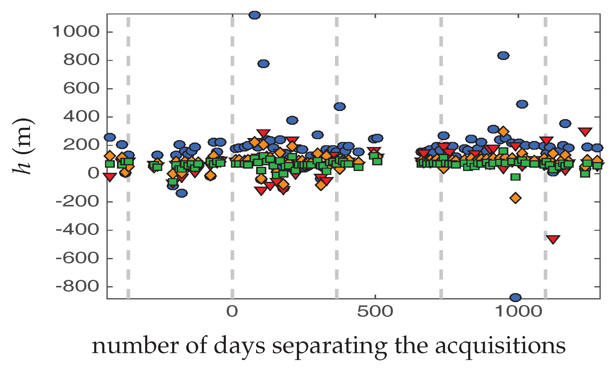
Figure 1 shows the variation in the baselines through time. The master image is the first image of the temporal stack that was studied in [12]. It has been acquired on the 24 January 2009 and is showed in red in Figure 1. After the launch of TanDEM-X (in June 2010), the maximal absolute baseline increases from 400 m to 900 m since both satellites acquired the images.
Two TSX-TDX PolInSAR images acquired over the same area supplement this dataset. They have been acquired on the 7 December 2015 and on the 18 December 2015 with the same acquisition parameters that can be found in Table 1, excepted in Stripmap Dual Receive Antennas (DRA) mode. The ground-pixel size is thus = 2.1 m and = 1.59 m and the resolution = 3 m and = 2 m in azimuth and ground range respectively. The PolInSAR baselines is −256 m for the 7 December 2015 image and −252 m for the 18 December 2015 image while the baseline between the two master images is 386 m.
2.2. The Studied Buildings
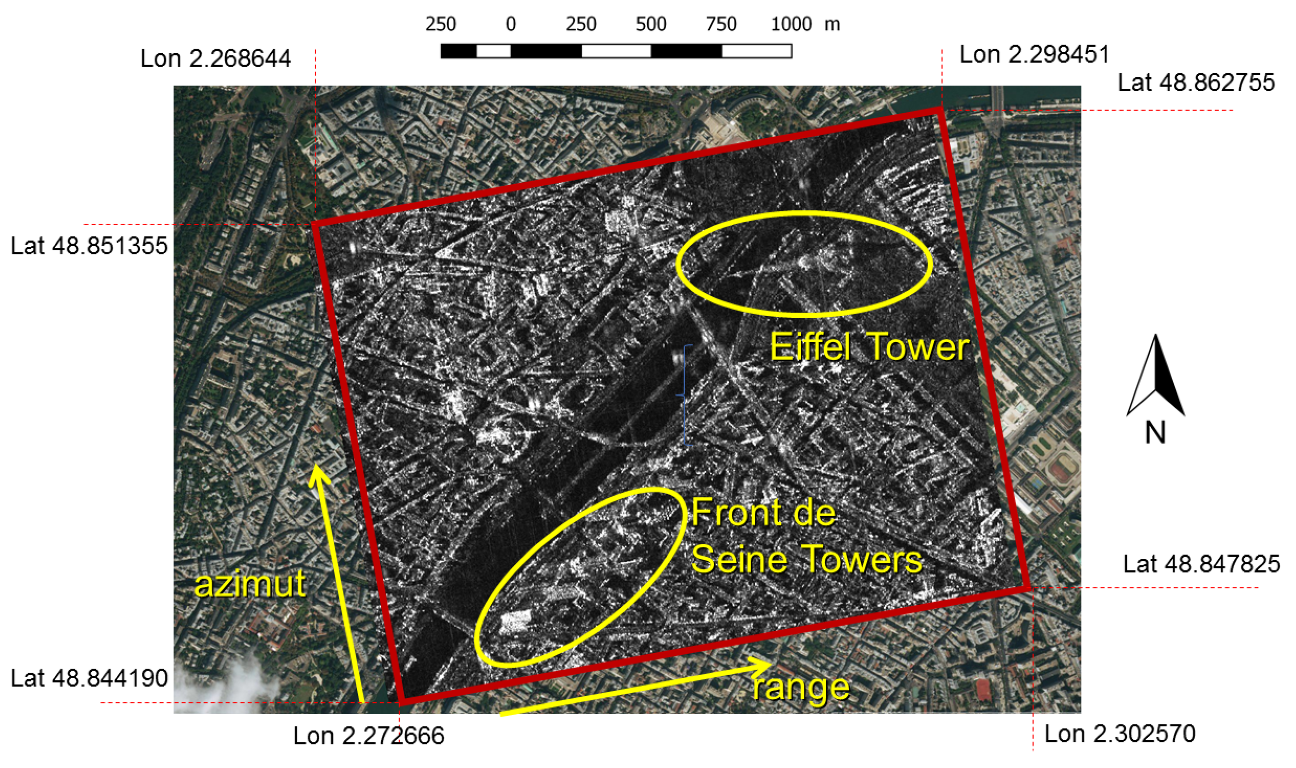
The buildings studied in this paper are known as Front de Seine elements. Front de Seine is a district in Paris, France, located along the river Seine in the 15th arrondissement at the south of the Eiffel Tower. It is one of the few districts in the city of Paris containing high rise buildings as they have mostly been constructed outside the city. It includes about 20 towers with varied designs, reaching nearly 100 m of height. The geographical location of the studied area is represented in Figure 2. This figure also links the SAR image azimuth/range geometry, in which all our SAR image extracts are represented with the geographical coordinates of the area.
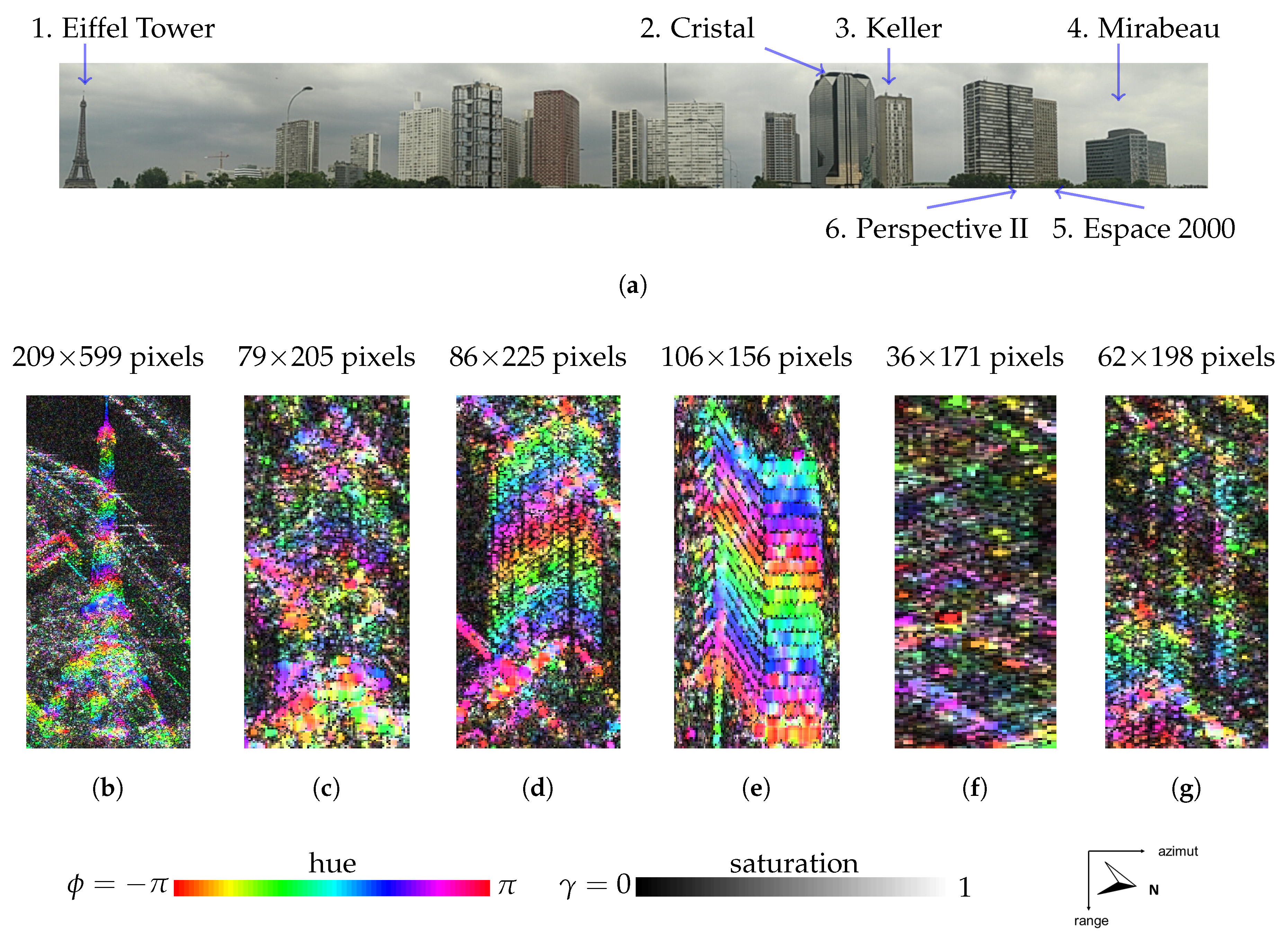
Six buildings were monitored during study: the emblematic Eiffel Tower and the Cristal, Keller, Mirabeau, Espace 2000 and Perspective II Towers. An optical images of the Front the Seine and the interferometric fringes over these buildings are represented in Figure 3. The SAR sensor images the layover between the south-west facade of the buildings and the ground.
As it can be seen in Figure 3, the studied buildings have different facade structure and material. The characteristics of these buildings is listed in Table 2. The Eiffel, Cristal, Keller and Mirabeau Tower are test buildings for the interferometric and the polarimetric experiences. In order to get buildings with the same orientation but different facade characteristics, the Espace 2000 and Perspective II Towers have been added to the polarimetric analysis. Due to the high variability in their facade, these two towers have a lower backscattered signal, as it can be seen in Figure 3f for the Espace 2000 Tower and in Figure 3g for the Perspective II Tower, on which interferometric fringes can mostly be seen in the middle and the extremities of the facade. Nevertheless, the Espace 2000 Tower has the same orientation than the Keller Tower even if the proportions of the buildings differ. The main facade of Perspective II Tower and the Cristal Tower have the same orientation, modulated by the varying shape of their facade.
For the Eiffel Tower, we can benefit from the comprehensive and expert knowledge of architects and structural engineers responsible for looking after and maintaining the monument and its facilities. La Société d’Exploitation de la Tour Eiffel (SETE) is the company running and maintaining the Eiffel Tower building. It has mandated the company OSMOS to monitor in situ the daily deformations.
It appears that the Eiffel tower is subjected to very complex deformation depending on weather conditions, mainly caused by three factors:
- The wind that makes the buildings oscillate in the perpendicular direction to the wind flow. Gustave Eiffel sized structure for the lateral oscillations due to wind up to 70 cm. However, oscillation amplitude records did not exceed 18 cm amplitude reached during the violent storm of December 1999. Hence, wind is not the most important deformation factor for this structure.
- The air temperature, that makes the iron and the concrete expend. The whole structures have then a vertical deformation. Depending on the temperature, the tower can elongate or shrink several centimeters. Given that the thermal expansion coefficient is approximately 10 m/(mK) for iron and concrete, buildings with a height of 100 m will have a 1 cm thermal expansion by 10 C temperature difference.
- The sunlight, that makes the side of the structures exposed to the sun expends more that the side of the structure that is in the shadow. The whole structures are thus bended in the direction opposite to the sun. The top of the Eiffel Tower can be shifted by 20 cm on a sunny day. This is thus the prevalent deformation effect for the studied buildings.
2.3. Multi-Channel SAR Estimation
InSAR and DInSAR images can be considered as multi-channel images after their corregistration. Four channels are acquired for PolSAR images, by the successive emission of wave in the H and V polarizations and the simultaneous reception of the two polarizations.
Thus, for these acquisition modes, each pixel of these images can be described by the scattering vector whose dimension N depends on the number of images constituting the dataset.
In the case of speckle, follows a circular-centered-normal distribution of covariance matrix [19]. The diagonal elements of the matrix is the power of the channel , while the off-diagonal element also depends on the degree of coherence between the k and j channel and the phase difference .
To estimate the covariance matrix, we use the maximum-likelihood estimator where the number of views L is the size of the sample used for the estimation. In the case of speckle, the rank of the covariance matrix is full and . The estimation sample can be chosen from neighborhood pixels, using non-local methods [20] or a temporal estimation [21] depending on the spatial and temporal variability of the studied targets.
If targets are deterministic as some very bright point-target present in urban areas, the rank of the covariance is 1. No averaging are needed to estimate the power or the phase difference, except to reduce the impact of residual thermal noise.
3. Measuring the Height by Interferometry
3.1. Methodology
3.1.1. SAR Interferometry Principle
Across-track SAR interferometry is based on the measurement of the phase difference between two SAR images acquired from different point of views, separated by a baseline . This phase difference is linked to the height of the scatterers h.
Single-pass interferometry enables to avoid temporal decorrelation effects and thus to limit the noise on the phase difference estimation. To perform single-pass acquisitions, two antennas have to be used conjointly, one emitting and the two receiving. This type of image can be acquired by satellite constellation composed of TSX and TDX, such as for the PolInSAR images used in this study. On the contrary, the same satellite can be used to acquired two images at two different moments. In this case, the acquisition corresponds to repeat-pass interferometry.
Single-pass interferometry is needed to guaranteed a high degree of coherence over vegetation and soils that decorrelate rapidly at X-band. Nevertheless, single-pass interferometry is very costly since the two satellites have to acquire conjointly. Due to operational constraint, TSX and TDX do not always flight in close formation. Moreover, the degree of coherence on urban structures and buildings is very high, even for acquisitions separated by more than four years: buildings are very stable structures leading to a very steady phase difference. Thus, it is possible to monitor buildings using repeat-pass interferometry, taking advantage of the long time series available.
In repeat-pass mode, the unwrapped phase difference can be linked to the height using the following equation [22]:
where is the repeat-pass interferometric factor. The minus sign account for the fact that the buildings are imaged in layover.
3.1.2. Unwrapping the Fringes
To obtain an interferometric result, the phase difference from the bottom to the top of the buildings, has to be estimated. Since the height of the studied buildings is often higher than the ambiguity height , the phase difference needs to be unwrapped.
In this study, the unwrapping has been performed on the whole building at ones by a comparison between the measured phase and a modeled phase [23]. The phase to unwrap is modeled by a linear phase having the same starting and ending point but a different number of fringes, and thus a different slope. The estimated number of fringes is then selected as the one maximizing the correlation between the measured and the modeled phases
This methodology enables to take into account the whole building during the phase estimation and not only some selected pixels in the image as it can be done in Permanent Scatterers (PS) framework [24]. Nevertheless, to guarantee a high accuracy of the phase, reference point at the bottom and the top of each building are chosen as Permanent Scatterers (PS), using a 0.5 threshold on the dispersion index for all the buildings. The dispersion index has been computed on the 98 images composing our inteferometric dataset.
Due to the lack of PS at the very bottom or very top of buildings, we have restricted the monitoring of the interferometric phase over a range of 85 m for the Cristal Tower, 90 m for the Keller Tower, and 68 m for the Mirabeau Tower. The Eiffel Tower is only monitored between the second floor and the antenna leading to a monitored height of 177 m. These heights are obtained by a monoscopic projection, defined by the vertical projection of the number of pixels between the PS: . They will be refereed as monoscopic reference to be compared by the inferferometric estimation. For the Cristal Tower, the limitation of the monitored height is due to the strong echoes at the base of the building whose secondary lobes leak the other pixels as it can been seen in Figure 3c. The base of the Keller Tower, represented in Figure 3d, has a different structure with a very low backscattering leading to the absence of PS.
Except 3 dates for the Eiffel Tower and 5 dates for the Cristal Tower, the phase could be unwrapped without user intervention (for the Eiffel Tower, the dates are the 15 November 2010, 20 January 2011 and 23 July 2012. For the Mirabeau Tower the 5 January 2010, 19 November 2008, 16 December 2011, 24 March 2013 and 23 July 2012). No averaging was needed, for the Eiffel, Keller and Mirabeau Towers. For the Cristal Tower, a five pixels azimuth boxcar filter has been used to estimate the phase. Avoiding averaging preserve the phase precision of the very bright scatterers present on the buildings.
3.2. Height Estimation Results for Two-Images-Repeat-Pass Interferometry
The height estimates are presented in Figure 4. This figure demonstrates that some estimated heights have very unrealistic values: the height of the Eiffel Tower has been estimated to more than one kilometer and negative heights are sometimes obtained for all the buildings. These unrealistic results show that the phase can not always be modeled alone by Equation (1), even if some previous studies have used it for measuring the exact height of the Eiffel Tower using only one repeat-pass interferometric pair [5,6].
After finer analysis of the results, these aberrant values appear are found for absolute values of below 0.2, when the baseline is smaller than 170 m and the phase difference is more sensible to deformation. Therefore, it can be assumed that the erroneous estimates come from the very small deformations that we have neglected in Equation (1). These very small deformations, of the order of millimeters, can exist on most structures and impact the repeat-pass interferometric phase, as already put forward for the Mirabeau bridge in [5]. This hypothesis is analyzed in Section 4 where the impact of the atmosphere on the phase will also be discussed.
This study shows nevertheless that an estimation of heights from a single repeat-pass couple of images can lead to false results. It is therefore necessary to use a more robust method for the elevation estimation from repeat-pass acquisitions as presented in the next section.
3.3. Height Estimation Results for Time-Series-Repeat-Pass Interferometry
As stated in Section 2.2, the studied building are deforming daily, in particular because of weather changes. Therefore, a deformation impacting the shape of the buildings between two difference acquisition date will impact the phase difference following:
For our data set, the term is constant and equal to whereas ranges between about 0.01 and 0.66. Neglecting 1 cm of deformation will generate between a 6 m error when and a 375 m error when . This can explain the unrealistic heights obtained in the previous section. It is, however, possible to measure the height of the buildings using the whole temporal stack in a different - and arguably more robust-way.
To this aim, the deformations at the different dates are assumed to be independent and to result in a Gaussian noise on the phase. Figure 5 shows the unwrapped phase difference given the multi-pass interferometric factor for the four buildings. The linear relationship between and is clearly visible. Using a linear regression between the unwrapped phase and , the height can be retrieved with a high degree of fit, as presented in Table 3. The heights estimated by linear regression show a good agreement with the reference heights of the buildings.
Only the unwrapped phases of the Cristal Tower seems to deviate from linear model: this buildings has the biggest difference between the reference and the regression height, and its coefficient of determination is the smallest. However, the deviation from the linear model occurs when the orthogonal baseline (and thus ) is small, as expected from Equation (2).
Since the phase is more impacted by the deformation when is small, large baselines could be considered as an easy way to measure the height without any impact of the deformation. However, when is high and thus the ambiguity height small, more fringes are visible on buildings and the phases are more difficult to unwrap automatically with the needed accuracy.
In this method, the fact that the height and the deformation account conjointly in the interferometric phase is overcome by the diversity in the baseline values. The linear regression based on nearly 100 images enables to limit errors in the height estimation.
4. Measuring the Deformation Trough Differential Interferometry
4.1. Methodology
Section 3.2 has demonstrated the non-negligible impact of deformations in height evaluations. This impact is due to the combination of the TSX 3 cm wavelength with the small baselines obtained with TSX orbital pattern. With the chosen master image, more than 90% of the baselines have an absolute value bellow 300 m.
This configuration enables a high accuracy on the measure of deformation using Equation (2) on an image by image basis. The phase difference is again measured using the methodology presented in Section 3.1.2. Equation (2) requires nevertheless the knowledge of the building height to measure the deformation. Thanks to our large time series, the height was estimated using only information contained in the SAR images, as presented in Section 3.3.
Even if the measured height are in good agreement with the reference height, Table 3 shows some noticeable difference. However, with the acquisition configuration, a one meter error on this height introduces an error on the deformation of m when and 1 mm when leading to centimeter precision in the worst case of the Cristal Tower. These centimeter precisions obtained with X-band images are a valuable assets for the remote monitoring of deformations.
The next section presents the results of the daily deformation estimation. Due to the multiple deformation factors presented in Section 2.2 and the time extend of our dataset, it is not possible to justify any temporal a priori on deformation, especially on a structure as complex as the Eiffel Tower. Thanks to the high accuracy obtainable with this dataset, deformations are computed for each acquisition date independently, in regard of the state of the buildings during the acquisition of the master image.
Since is the phase difference between the bottom and to top of the buildings, unwrapped globally on the whole building facades, it is implicitly assumed that the deformation is constant along the vertical axis of the building. Note that the deformation are measured in the Line of Sight direction and here are not reprojected since we do not assume any direction for the deformations.
4.2. Deformation Estimation Results
The estimated deformations are represented in Figure 6. The deformations of the Eiffel Tower show a very high variability as presented in Figure 6a. On the contrary, Figure 6d shows the annual periodicity of the deformations of the Mirabeau Tower. Except for some date, an annual periodicity can be seen in Figure 6b, for the deformations of the Cristal Tower for the years 2008 and 2009. This periodicity is unclear for the other years even if the deformation are smaller in winter than in summer. The deformations of the Keller Tower are also minimal in winter and maximal in summer but the variability of the measured deformation that can be observed in Figure 6c lead to an unclear annual cycle.
The annual periodicity of the deformation measured on the Mirabeau Towers would indicate thermal expansion due to the temperature as the major cause of the deformation. The more important dispersion observed in the deformation of the other towers underline the numerous deformation sources For example, under the sun light action, the buildings bend in direction the opposite to the sun. The sunshine can change the amplitude and the direction of the deformation on a daily basis. Moreover, even a small rain shower reset the buildings back in their original position, changing their deformation state at the time of the acquisition.
On top of the several sources of deformation that can co-exist, the measurement can still be impacted by noise. The low backscattering on the Cristal Tower required some averaging and to increase the threshold value on the PS selection. This is why a special effort has been made to validate and cross-check our measurements with other data, the first of which are weather parameters.
4.3. Analysis of the Estimated Deformation
4.3.1. Comparison with Weather Data
All parameter values have been collected from the archives of the Meteo France weather data [25,26]. They have been recorded by the Paris weather station situated in the parc Montsouris, south east from the studied area. Four weather parameters have been used to validate our deformation measurements:
- The time between the acquisition and sun set , which enables to account for the periodicity in the measured deformations.
- The minimal temperature the day of the acquisition , linked to the thermal expansion in the measured deformation.
- The number of sunny hours during the acquisition day , that can be linked to the bending of the building caused by sunlight.
- The maximal gust during the hour of the acquisition , that can account for the deformation due to wind.
The normalized correlation between the weather data and the deformations, listed in Table 4, shows different result for the Mirabeau tower compared to the three other structures.
For the Mirabeau Tower, the high normalized correlation between the measured deformation and the duration between the acquisition time and the sunset shows well the periodicity of the measured deformations. The sign minus is explained by the fact that the deformation are minimal in winter, when the sunset occurs before the acquisition and thus . These deformations seem mainly due to the thermal expansion and the sunlight, given the high correlation with and the medium correlation with . There is no correlation with . Indeed, structures respond very quickly to wind forcing and no records of the wind information precisely at the acquisition time are available.
For the other buildings, the correlation with the time between the acquisition and the sunset is low, highlighting the absence of periodicity in the measured deformations. Thermal expansion seems to be the major origin of the measured deformation. However, the normalized correlation between the measured deformation and minimal temperature is around 0.5, meaning that the temperature does not explain alone the deformations. The correlation with the sunlight values is smaller than expected especially for the Eiffel Tower for which it is the principal deformation cause according to experts. The difference between the behavior of the Mirabeau Tower and the other towers can be explained by internal structure informations to which we do not have access, or by the different impact of other buildings adjacent to the site and shadow effects.
The measured correlations underline the exogenous nature of the phase anomaly leading the unrealistic InSAR heights. However, the validation process does not allow to separate atmospheric changes impacting the phase and recorded through weather parameters from buildings deformations due to weather modifications. The estimated deformations have thus been compared to in situ measurements in Section 4.3.2 and the maximum error potentially induced by the atmosphere is assessed in Section 4.4.
4.3.2. Comparison with In Situ Measurements
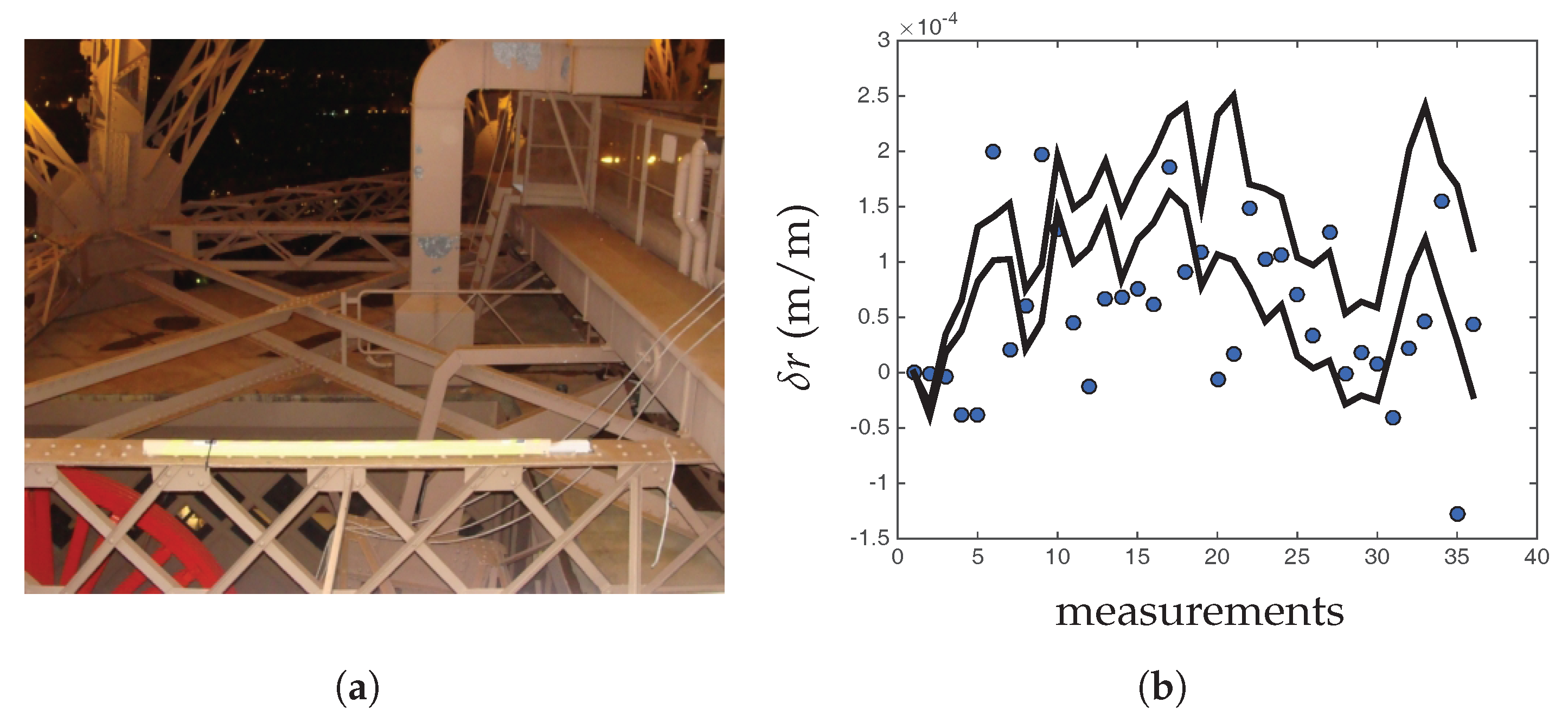
The Societe d’Exploitation de la Tour Eiffel (SETE) has charged the company OSMOS to monitor routinely the deformations of the Eiffel Tower thanks to their optical strand system pictured in Figure 7a. This process is based on the principle of the modulation of light intensity by measuring analog attenuation along an optical fibre coil. The deformation are average on a measurement interval leading a very low variability of the measurement. For over 20 years, OSMOS has monitored the stability of the main structural elements of the Eiffel towers, through several local deformation measurements, performed at numerous locations on the structure.
The SETE granted us access to 36 deformation measures for 8 optical strands installed at the first floor of the Eiffel Tower, at the specific times of SAR acquisitions. Two optical strands are installed horizontally on each side of the tower, one on the exterior part of the first floor and one on the interior part. The minimum and the maximum values for the optical strands are represented in Figure 7b. The observed variation are caused to anisotropic deformation leading to bigger deformation on some sides of the Eiffel Tower than the others. These differences are more likely to be due to deformation induced by the sunlight, since only one side of the structure is illuminated.
In order to compare the same physical quantities, we have converted our measurements into linear deformation, assuming that the main deformation axis is vertical, and dividing the total deformation by the height of the turn portion on which deformation is estimated. Figure 7b represents the mean linear deformation measured by DInSAR, as well as the maximal and minimal linear deformation measured by the optical strands.
Even if the chosen strands are not in the studied area, Figure 7b shows that the order of magnitude of the DInSAR deformations agree with the optical strands measurements. A quarter of the DInSAR deformation are between the minimal and the maximal optical strand measured deformations.
The comparison of our global deformation with the local deformation obtained by the optical strand is not an individual validation of our measurement. However, the orders of magnitude are valid, although this comparison has been performed on the Eiffel Tower, which is the building showing the largest and the most chaotic deformation pattern. Moreover, we measured linear deformations by making a very coarse hypothesis on the deformation, assuming that it is linear, and oriented along a vertical axis. However, we know that is certainly not the case, and that it is difficult to extrapolate a point measure to a global homoegenous linear measure. Therefore, the relatively good agreement between the values of the DInSAR deformations and the optical-strand deformations validate the developed process chain. It also support our hypothesis that the unrealistic-InSAR height are due to deformations of the buildings between the acquisitions.
Neglecting the impact of the atmosphere limits however the accuracy of the estimated DInSAR deformation since variation in the optical path length due to the atmosphere can wrongly be attributed to scatterers deformation [27]. The impact of the atmosphere is thus discussed in the next section.
4.4. Discussion on the Impact of the Atmosphere on the Precision of the Estimated Deformation
The fact that waves backscattered by the base of the buildings propagate trough different atmospheric conditions than the waves backscattered by the top of the buildings will impact the phase difference. The unwrapped phase differences as computed in this study will thus depend on the height and the deformation of the buildings, but also on the atmospheric delay. In this section, we estimate the maximum deformation error introduced by neglecting the changes in atmospheric condition.
Two layers of the atmosphere can impact our deformation measurement: the ionosphere and the troposphere. At X-band, the ionospheric delay is very small and the ionosphere variation have a large spatial extend, impacting the same way waves backscattered by the base and the top of the buildings. The error induced by the ionosphere can thus be neglected.
To assess the tropospheric delay variation between the top and the ground of the studied buildings, we model the tropospheric delay as exponentially decreasing with the height:
where is the global tropospheric delay, also called Zenith Path Delay (ZPD), the look angle and H is the height of the troposphere. As the DLR teams in [28], we are taking H = 6000 m. The Zenith path delay can be measured from ground stations of the Global Navigation Satellite System. For the EUREF Permanent Network station at Marne la Vallée ( = 160 m), the smallest ZPD is 2340 mm and occurs in winter while the biggest ZPD is 2440 mm and occurs in summer.
For the Eiffel Tower, the residual delay between the pole and the second floor is:
For the Mirabeau Tower, located at an altitude of 33 m with a height of 70 m, the residual tropospheric delay is −1.6 mm. The atmospheric delay results in millimeter error for the DInSAR deformation measurement.
This error on the deformation measurement has the same order of magnitude than the one induced by a one meter error on the height. Along with the residual error on the PS phases, the precision of the estimated deformation is below 5 mm, which is below the deformation variations illustrated in Figure 6.
This section demonstrates that the X-band is favorable to the measurement of complex structural deformations at different points of a building, given its height. This height can be assumed to be known elsewhere, or calculated using the whole data stack according to the method of the previous section. Errors of 1 m on the building height lead to negligible inaccuracies in the final deformation estimate, as well as the noncompensation of atmospheric effects locally between the top and bottom of the building.
The deformation measured using SAR images is linked with the scattering mechanisms involved. However, in urban area and particularly at X-band, these mechanisms can be difficult to interpret. The next section investigates the contribution of polarimetry to refine the analysis of the scattering mechanisms in urban area that could lead to a better understanding of the structure of buildings as seen by the SAR sensor.
5. Polarimetric Analysis
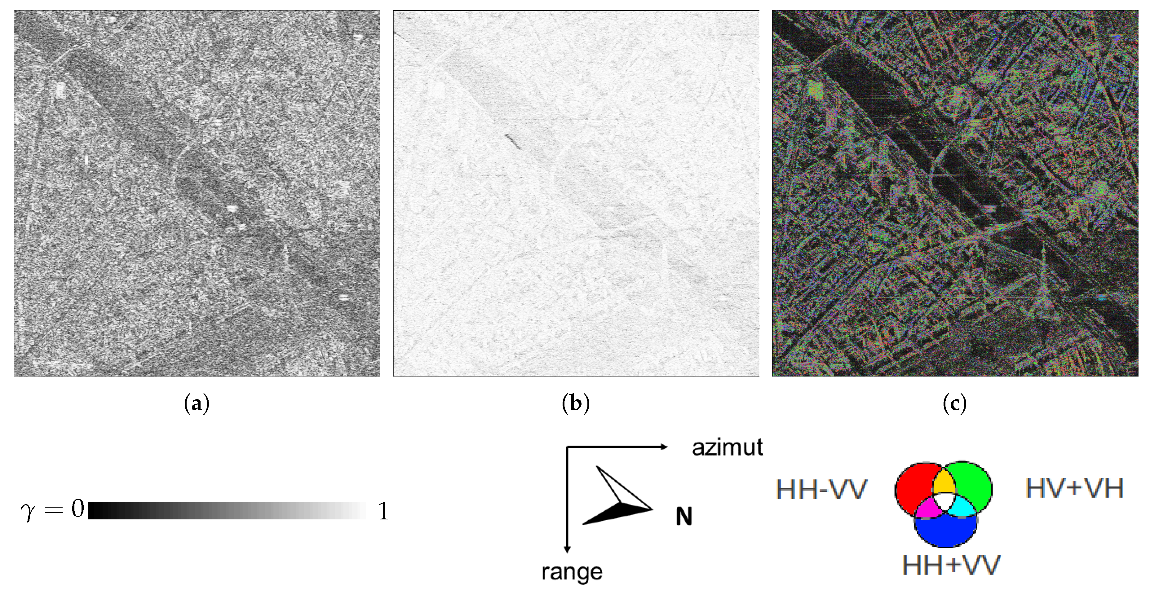
Polarimetric mode provides valuable information on scene materials, geometry and the nature of the electromagnetic scattering mechanism involved. However, polarimetric images are often acquired at coarser resolutions. Up to now, polarimetry has been used for classification and analysis purpose, or in combination with interferometry, mainly trough coherence optimization for estimating different scattering phase centers in a given resolution cell, or for increasing the number of permanent scatterers selected to estimate deformations. Today, studies on benefits of polarimetry over urban areas have been limited, mainly by the lack of real polarimetric data at high resolution. Here, our data set includes two PolInSAR Tandem-X acquisitions in a stripmap 2 × 3 m resolution. Thus, the dataset corresponds to four polarimetric images. Only one temporal baseline is available, and therefore, analysis is limited to first investigations. This study concerns first the benefit of polarimetry for repeat-pass interferometry, then the polarimetric analysis of buildings. One of the polarimetric image is represented in the Pauli basis in Figure 8 on the left, and one of the corresponding interferogram acquired in the repeat pass mode is shown on the right.
5.1. Benefit of Polarimetry for Repeat-Pass Interferometry
Both image couples of Tandem-X have been co-registered together, and orbital fringes have been removed between the two dates. Then, coherence matrices have been estimated. Since ambiguity height is very small, about 20 m, interferometric phase variations along range are very fast. Since a range average would mix together very different interferometric phases, coherence matrices have been estimated by an average only in the azimuth direction over 5 pixels. Optimization of coherence has then been applied according to [29]. This coherence leads to find very higher coherence levels. The resulting coherence distributions are plotted in Figure 9. Coherence are estimated using the same estimation of only five pixels. In HV and VH polarimetric channels, coherence are very slightly below what is obtained with co-polarimetric channels for coherence values higher than 0.7. The reverse of this can be seen for low coherence values, for which HV and VH lead to coherence slightly higher than HH and VV.
However, what is clear on this figure is that optimized coherence is considerably greater than all original polarimetric channels. That means that for a given threshold on the coherence level, the corresponding numbers of selected scatterers will be greatly improved.
Unfortunately, it is very difficult to prove that the differential interferometric phase is better estimated, due to the strong variations. It is nevertheless interesting to know which kind of polarimetric mechanism lead to the highest coherence. To this aim, we have represented as a colored composition the absolute value of the optimal polarimetric mechanism components in the Pauli basis. Thus, the interferometric coherence in HH polarization is represented in Figure 10 on the left, interferometric coherence obtained in the optimal polarization if shown on the middle; on the right, an intensity image is colored with the three component magnitude of the optimal mechanism, expressed in the Pauli basis.
In this figure, it appears that the optimal mechanisms are not necessarily those that lead to the maximum intensities. The strong mechanisms in HV and VH are often visible; Moreover, the optimal mechanisms vary greatly from one building to another. On the Mirabeau tower, the green color is predominant; On the Keller tower one face appears mostly in HH−VV and the other in HH+VV.
5.2. Benefit of Polarimetry for Building Monitoring
5.2.1. Main Investigation: Orientations and Materials
Most polarimetric classification methods rely on the study of second-order parameters, estimated from several statistical samples.
Generally, a spatial estimation is made by choosing the samples either in an immediate neighbourhood or in other areas of the image. Recently, it has been demonstrated that for metric resolution images, a polarimetric spatial estimation, even if carried out carefully, leads to a very high entropy, whereas temporal estimation makes it possible to find low entropies on bright point-like scatterers [21]. This means that for these pixels, only a temporal estimation is able to characterize the scattering process on a deterministic point of view. Since we are interested in parameters for industrial structures, or building elements, we restrain the analysis of these deterministic processes.
Two properties are of interest in the analysis of structures and their possible deformation:
- The orientation of buildings. Indeed, our measurements of local deformations on buildings presuppose that this deformation is mainly in the vertical direction. However, if a scattering structure element has a different orientation, the axis of deformation will also be different. It is interesting firstly to be able to identify these cases and in a second step to use this information to project the measured deformation in the structure direction.
- Building materials. Again, this is crucial for a potential deformation measure: the effects of thermal expansion which seems to be predominant deformation effect measured with DInSAR data, depend on the material.
Several studies are concerned with the contribution of polarimetry to the evaluation of these characteristics. In particular, the potential of polarimetry to extract orientation and dielectric propertied of individual coherent scatterers has been investigated in [30]. However, up to now, due to the lack of real polarimetric data at high resolution, they mainly concern simulation [31]. Generic behaviours were deduced, in particular the backscattering seems to be sensitive to the dielectric permittivity of the buildings [32].
Several deterministic approaches are possible, for example but not exhaustive, Huynen parameters, Cameron’s classification, or research efforts in optical ellipsometry, for example polar decompositions. The later are interesting because they do not consider the metallic hypothesis: they are adapted equally well to dielectric structures, which is not the case for the first two which more specifically address the geometry of the PEC targets and do not take into consideration the effects on materials. Note that ellipsometry has been more applied to surface scattering, but has already been used frequently to determine the effects of orientations, such as those present in biological tissue fibers [33].
Therefore, in order to investigate the potential of polarimetry in the characterization of deformations, our approach is as follows:
- First, the both polarimetric acquisitions have been co-registered together at a sub-pixel precision, using [34].
- For each pixel, we applied to the Sinclair matrix the polar decomposition described in [35], to be able to describe diattenuation and retardance properties. Diattenuation concerns only the change in the amplitudes of the components of the electric field vector, whereas the retarder changes only the phases of components of the electric-field vector.
- We extract the two main parameters, retardance and diattenuation, as well as the orientation of the axes of the two main Stokes vectors (maximum retardance axis and maximum diattenuation axis).
The resulting parameters are analyzed for the four available polarimetric images.
5.2.2. Dedicated Ground Truth
This study has been performed on all buildings presented in Section 2. The five Front-de-Seine buildings are represented in Figure 11. The towers are represented first by their faces in the line of sight of the radar in Figure 11a. In Figure 11b, we represent the faces that are not seen by the radar. In this view, the buildings appear in the same order of appearance as in the polarimetric radar image represented in Figure 11c.
The particularities of these polarimetric images reside in the wavelength and the particular spatial resolution. These features create new processing difficulties. At this wavelength of 3 cm, scattering mechanisms are very anisotropic, and it is very hard to predict which kind of elements will dominate the signal response, because several interactions can occur with very small objects. However, it is interesting to check how and to what extent we can deduce information about the orientation of the main structuring element such as main beams of the Eiffel Tower or main fronts of more conventional towers, from the TerraSAR-X polarimetric mode.
To this aim, 3D representation of the structures under study were used to constitute a ground truth of the orientations of our structures. From these models, we extract the orientation vector of uni-axial object:
- For the five towers, we consider any horizontal vectors belonging to each vertical face including window sills, vertical ducts, floor separations, balcony edging profile, etc.
- For the Eiffel tower, we consider all principal beams of the structure.
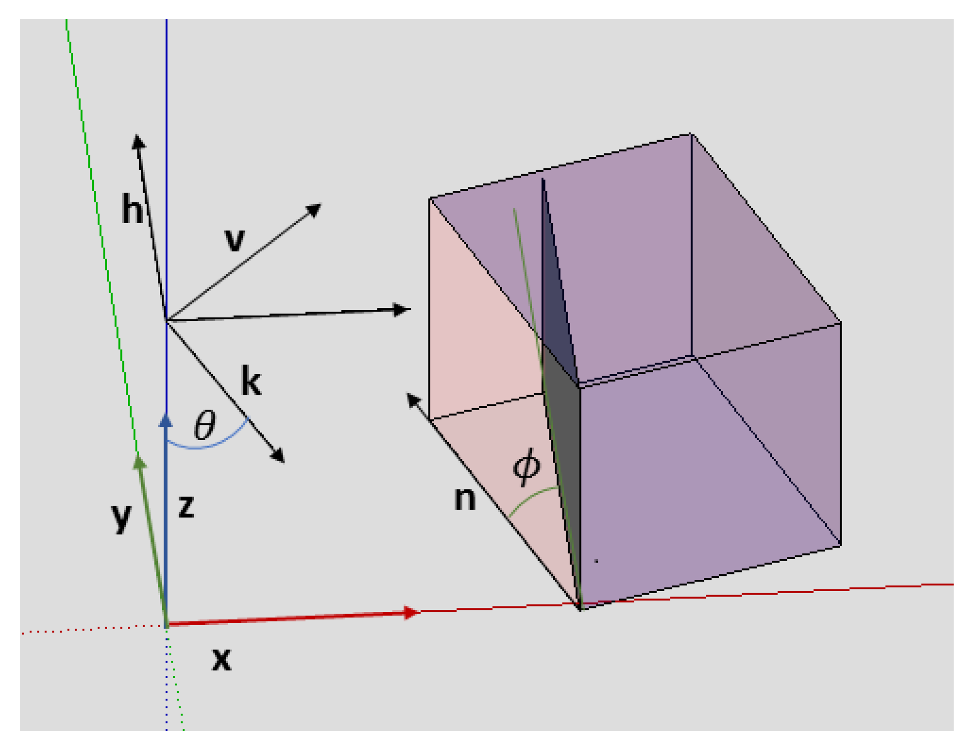
In Figure 12, we explain the notations for a horizontal element of a wall oriented with an angle with respect to the trajectory.
To calculate the theoretical orientation of any vector of our ground truth in the wave plane, it is sufficient to first calculate its projection in this wave-plane by . In the particular case represented in Figure 12 where is horizontal:
Then the orientation angle formed between this projection and the horizontal polarimetric vector , can be found by . It should be noted that only a vertical vector has a simple expression of its orientation, which remains vertical. The orientation of any horizontal vector projected in the wave plane is not exactly its azimuth angle, as soon as the incidence is not zero. Indeed, the literal expression leads to an influence of the angle of incidence :
However, the difference between azimuth and polarimetric angle is not very important for low incidence we are considering. The relation between and has been plotted in Figure 13 for several incidence angles ; the incidence angle of the images is 34.
5.2.3. Results
We present now the orientation distributions found over main fronts of our five buidings, and compare them with the true orientations found for horizontal elements of the walls.
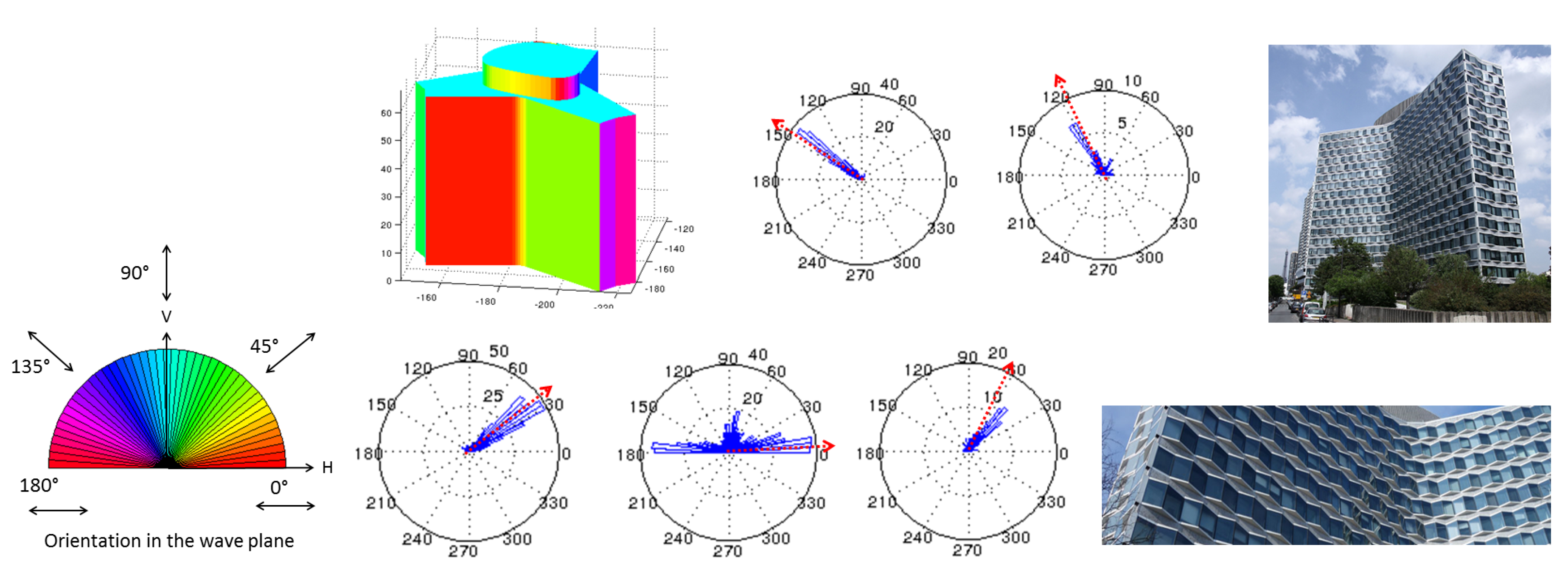
Mirabeau Tower
First, results obtained on the Mirabeau Tower are shown in Figure 14. Five different facades with different orientations are visible on the image. Resulting orientation angles are very well correlated with our ground truth, represented by the red arrows in the charts, and by the colored representation of the 3D model. They show clearly the influence of facade orientation respective to azimuth direction. The orientations have been computed for the four polarimetric images. They do not differ a lot from one polarimetric to the other one, except for the wall exactly aligned with the azimuth. Only in this case, small differences can be noticed between the strictly monostatic acquisitions, and the quasi-monostatic ones where transmitter and receiver belong to the two different sensors TSX and TDX.
Note that the facades are not strictly plane, as the picture shows: the faces therefore have a variability of orientations that can explain the variance of our estimates.
Espace 2000 and Keller Towers
In Figure 15, we analyze two different buildings, the Espace 2000 Tower (Building 5) and the Keller (Building 3) Tower which facade have very similar global orientations, but different scattering. Estimations made on the Keller Tower show that both facades include the two main orientations found in the ground truth. The facade photo reveals that window frames include both directions. They are probably the cause of trihedral effects and could explain the strong signal scattered by this building. In any case, both main directions are retrieved in the polarimetric angle estimation. Orientation values estimated over the Espace 2000 Tower are more dispersed. Picture reveals that the small balconies have much more complex shapes. Principal orientations remain, but with more variability.
Perspective II and Cristal Towers
Figure 16 shows results for more complex buildings: the Perspective II and Cristal towers. Once again, the main orientations are retrieved. The Cristal tower is the one that generates the bigger variability. This is probably due to the fact that the Cristal tower has also a very low backscattered signal, because it is made on glass that exhibits a very high absorptivity at X-band. Thus, the estimation of the orientation is very noisy. For Perspective II, one of the privileged orientations is found for both main facades.
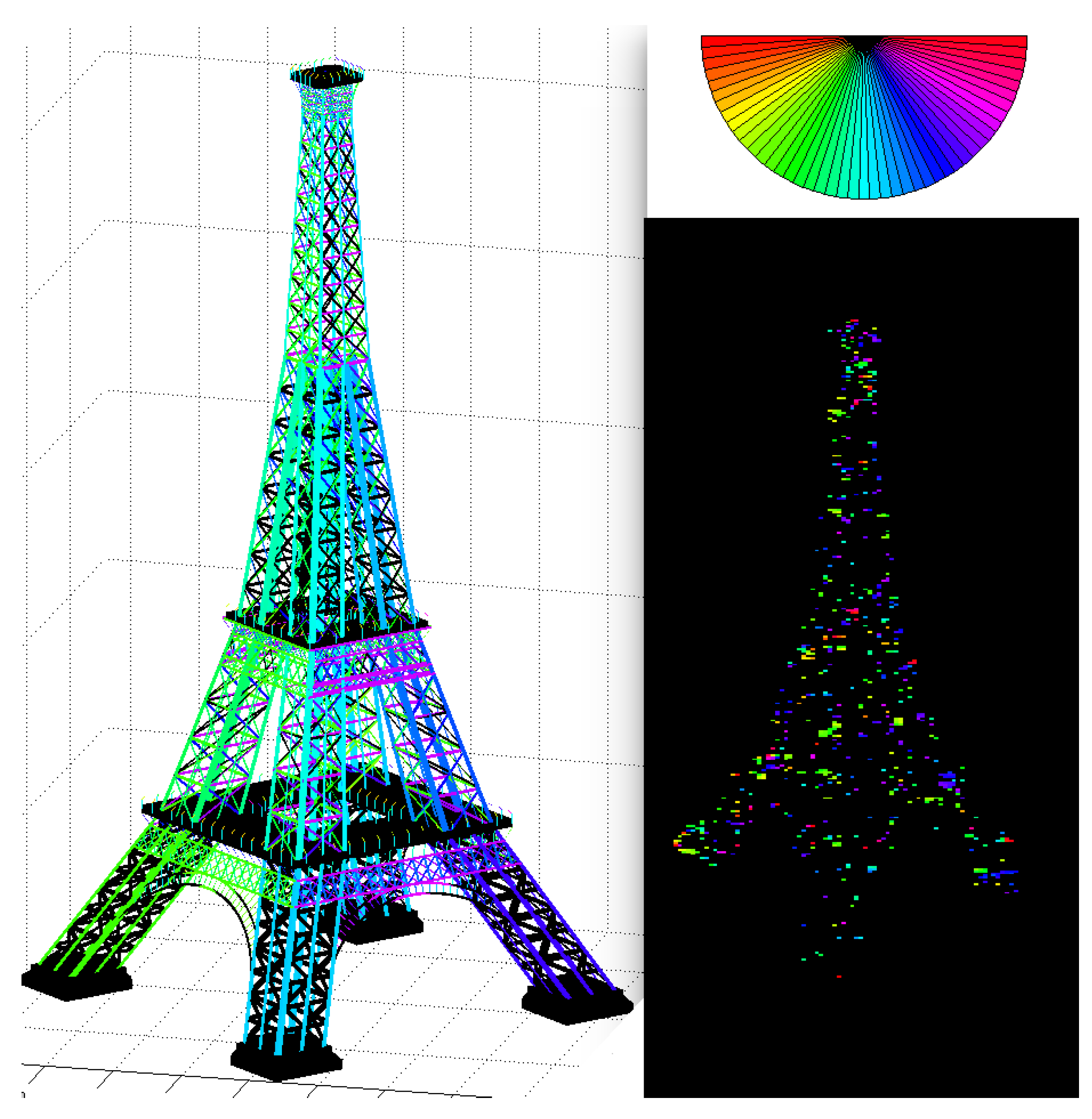
Eiffel Tower
For the Eiffel Tower, orientation effects are very chaotic. The structure is very difficult to describe, and as mentioned previously, polarimetric return is hard to anticipate. We have thus restricted comparison with ground truth to pixels whose estimated orientation are very similar among the four acquisitions. To check this point, we have computed the second circular statistical moment to select only pixels whose orientation homogeneity is at least 80%. At a coarse scale, these estimations are correlated to those of the ground truth. Results are shown on Figure 17.
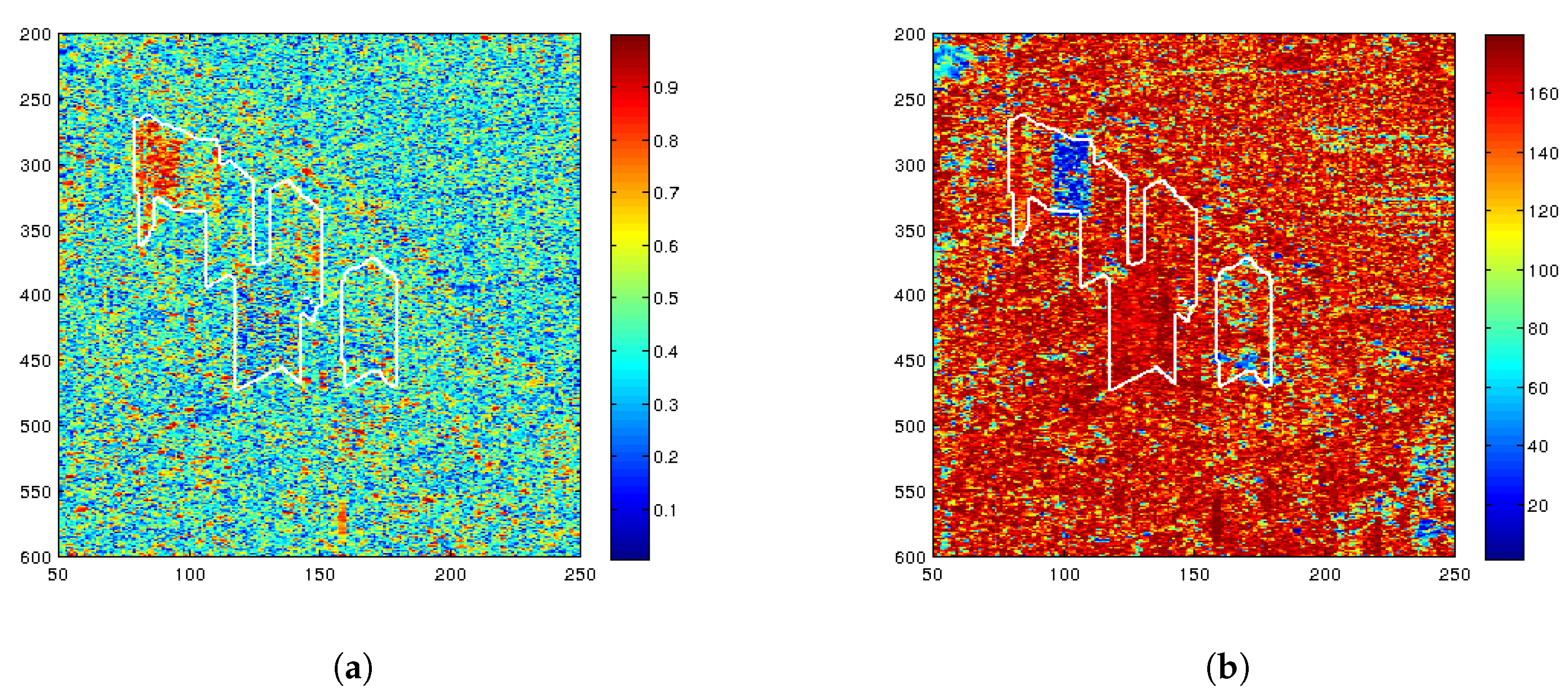
Finally, diattenuation and retardance have been computed. They are represented in Figure 18. Retardance is very sensible to the parity of number of bounces involved in the scattering process. It shows that the facade of the Mirabeau tower aligned with the azimuth involves a lot of local double-bounce scattering on the windowsills. These double bounce mechanisms disappear when an angle is introduced between the facade and the azimuth axis. The value of the diattenuation differs even for buildings having the same general orientations. This difference may be due either to differences in materials and permittivity, or to differences in local geometries in structures.
6. Conclusions
A careful analysis of a TerraSAR-X dataset over urban area has been presented in this article. The major assets of this sensor for urban area are its fine resolution and its agility enabling to acquired images in different modes. The studied dataset combines 98 for InSAR/DInSAR images acquired during four years and two PolInSAR acquisitions. Using this dataset we could quantify the contributions, as well as the underlying difficulties, of each mode.
Concerning the updating of building elevations, we showed that the repeat-pass InSAR mode leads to a coherence high enough to use the interferometric phase on the buildings, even with three years separating the acquisitions. However, more than one repeat-pass pair is needed to get reliable height estimated since even the slight daily building deformations can have a great impact of elevation measurement. We have proposed an efficient method to make the height measurement more robust by using the entire time series.
Thanks to this sensibility to buildings deformation due to the TSX wavelength and resolution, we have also demonstrated that it becomes possible to use the DInSAR mode to monitor the building deformations. This has been done without making any assumption on the deformation processes. This was particularly useful to estimate non-linear deformations, such as for the Eiffel Tower, whose deformation behavior is very complex to model. For the Eiffel Tower, we measured deformation up to 4 cm over the time series and we estimated deformation about 1 cm for the three other studied buildings. Our deformation estimations were compared with local in situ measurements and were of the same order of magnitude. Our estimations were also correlated to weather data. This validation has proven that a centimeter precision can be achieved even when neglecting the atmosphere. It has also shown that building deformation patterns observed differ widely between profiles.
Finally, we have investigated the benefit of the polarimetric mode for building monitoring. As in previous study, the polarimetric coherence optimization has been proven to be very effective to increase the coherence level. Nevertheless, the small polarimetric dataset and the small ambiguity height limit the use of the interferometric phase for repeat pass deformation measurement. In order to measure information about the geometry and the materials from polarimetric images, the deterministic analysis seems to be appropriate. Indeed, at this wavelength and resolution range, polarimeteric signals are stable among time but are not reproducible between neighboring pixels. The polarimetric return is large part dominated by orientation effects. We have shown that the orientations of the main attenuation axis are very well correlated with the orientation of the vertical facades with respect to the azimuth axis. Results are still limited by the resolution loss in the polarimetric mode, but are encouraging for future sensors. Indeed, the gains made by the increasing resolutions, already demonstrated in the single-pol modes, make it possible to envisage polarimetry for new kinds of applications: geometry and complexity of facades and structures.
This paper provides some reasons to be optimistic for the use of X-band very high resolution sensors for measuring and analysing the deformation of the structures. To improve the resolution scale of the deformation estimation, single-pass mode and repeat-pass mode could be combined. Deformations for every resolution cell at the different elevations of the buildings could be estimated, taking fully advantage of the TSX resolution. Ground and building deformations could thus be separated. By coupling the deformation measurement to the polarimetric analysis could first help to improve the robustness of the deformation estimation by giving the orientation of the scatterers as seen by the sensor and thus the direction of the measured deformation.
Acknowledgments
The first author was partially supported by a PhD grant from the DGA (Direction Generale de l’Armement). The authors want to acknowledge the SETE for their disclosure of optical strand data. Thanks to OSMOS and particularly to Constant Choqueuse and François-Baptiste Cartiaux for sharing their knowledge on the structure deformation and helped with the optical strand validation. The authors would also like to acknowledge Elise Nkassa for the collection of the weather data in Telecom Paris Tech.
Author Contributions
Flora Weissgerber and Elise Colin-Koeniguer were the main authors of the paper. Jean-Marie Nicolas conceived the InSAR and DInSAR experiment. Flora Weissgerber gathered the data, performed the InSAR and DInSAR experiments as well as the validation process for these results. Elise Colin-Koeniguer has conceived and performed the PolSAR experiments and analyzed the results conjointly with Nicolas Trouvé.
Conflicts of Interest
The authors declare no conflict of interest. The founding sponsors had no role in the design of the study; in the collection, analyses, or interpretation of data and in the writing of the manuscript. In accordance to the SETE guidelines, the dates of the comparison between the optical strands and the DInSAR deformations are not disclosed.
Abbreviations
The following abbreviations are used in this manuscript.
| InSAR | interferometric SAR |
| DInSAR | differential interferometric SAR |
| PolSAR | polarimetric SAR |
| PS | permanent scatterer |
| SETE | Société d’Exploitation de la Tour Eiffel |
| TSX | TerraSAR-X |
| TDX | TanDEM-X |
| VHR | Very High Resolution |
| ZPD | Zenith Path Delay |
References
- Bonano, M.; Manunta, M.; Pepe, A.; Paglia, L.; Lanari, R. From previous C-band to new X-band SAR systems: Assessment of the DInSAR mapping improvement for deformation time-series retrieval in urban areas. IEEE Trans. Geosci. Remote Sens. 2013, 51, 1973–1984. [Google Scholar] [CrossRef]
- Tison, C.; Tupin, F.; Maitre, H. Extraction of Urban Elevation Models form High Resolution Interferometric SAR Images. In Proceedings of the 5th European Conference on Synthetic Aperture Radar, Ulm, Germany, 25–27 May 2004; pp. 411–414. [Google Scholar]
- Thiele, A.; Thoennessen, U.; Cadario, E.; Schulz, K.; Soergel, U. Building recognition from multi-aspect high-resolution interferometric SAR data in urban areas. IEEE Trans. Geosci. Remote Sens. 2007, 45, 3583–3593. [Google Scholar] [CrossRef]
- Colin-Koeniguer, E.; Trouve, N. Performance of building height estimation using high-resolution PolInSAR images. IEEE Trans. Geosci. Remote Sens. 2014, 52, 5870–5879. [Google Scholar] [CrossRef]
- Bamler, R.; Eineder, M.; Adam, N.; Zhu, X.; Gernhardt, S. Interferometric potential of high resolution spaceborne SAR. Photogramm. Fernerkund. Geoinf. 2009, 2009, 407–419. [Google Scholar] [CrossRef]
- Brcic, R.; Eineder, M.; Bamler, R.; Steinbrecher, U.; Schulze, D.; Metzig, R.; Papathanassiou, K.P.; Nagler, T.; Mueller, F.; Suess, M. Delta-k wideband SAR interferometry for DEM generation and PSI using Terrasar-X. In Proceedings of the ESA Proc. FRINGE, Frascati, Italy, 30 November–4 December 2009. [Google Scholar]
- Ferretti, A.; Prati, C.; Rocca, F. Nonlinear Subsidence Rate Estimation Using Permanent Scatterers in Differential SAR Interferometry. IEEE Trans. Geosci. Remote Sens. 2000, 38, 2202–2212. [Google Scholar] [CrossRef]
- Ferretti, A.; Ferrucci, F.; Prati, C.; Rocca, F. SAR Analysis of Building Collapse by means of Permanent Scatterers Technique. In Proceedings of the IEEE 2000 International Geoscience and Remote Sensing Symposium. Taking the Pulse of the Planet: The Role of Remote Sensing in Managing the Environment, Honolulu, HI, USA, 24–28 July 2000; Volume 7, pp. 3219–3221. [Google Scholar]
- Zeni, G.; Bonano, M.; Casu, F.; Manunta, M.; Manzo, M.; Marsella, M.; Pepe, A.; Lanari, R. Long-term deformation analysis of historical buildings through the advanced SBAS-DInSAR technique: The case study of the city of Rome, Italy. J. Geophys. Eng. 2011, 8, S1. [Google Scholar] [CrossRef]
- Fornaro, G.; Pauciullo, A.; Reale, D.; Zhu, X.; Bamler, R. Peculiarities of Urban Area Analysis With Very High Resolution Interferometric SAR Data. In Proceedings of the JURSE 2011—Joint Urban Remote Sensing Event, Munich, Germany, 11–13 April 2011; pp. 185–188. [Google Scholar]
- Yang, K.; Yan, L.; Huang, G.; Chen, C.; Wu, Z. Monitoring building deformation with InSAR: Experiments and validation. Sensors 2016, 16, 2182. [Google Scholar] [CrossRef] [PubMed]
- Weissgerber, F.; Nicolas, J.M.; Colin-koeniguer, E.; Trouvé, N. Mesure de la dilatation thermique de la Tour Eiffel par interférométrie RSO differentielle. In Proceedings of the GRETSI, Lyon, France, 8–11 September 2015. [Google Scholar]
- Moriyama, T.; Yamaguchi, Y.; Uratsuka, S.; Umehara, T.; Maeno, H.; Satake, M.; Nadai, A.; Nakamura, K. A study on polarimetric correlation coefficient for feature extraction of polarimetric SAR data. IEICE Trans. Commun. 2005, 88, 2353–2361. [Google Scholar] [CrossRef]
- Cloude, S. Polarisation: Applications in Remote Sensing; Oxford University Press: Oxford, UK, 2010. [Google Scholar]
- Iribe, K.; Sato, M. Analysis of polarization orientation angle shifts by artificial structures. IEEE Trans. Geosci. Remote Sens. 2007, 45, 3417–3425. [Google Scholar] [CrossRef]
- Duquenoy, M.; Ovarlez, J.; Morisseau, C.; Vieillard, G.; Ferro-Famil, L.; Pottier, E. Supervised classification by neural networks using polarimetric time-frequency signatures. In Proceedings of the 2009 IEEE International Geoscience and Remote Sensing Symposium, Cape Town, South Africa, 12–17 July 2009; Volume 4, p. IV-438. [Google Scholar]
- Pipia, L.; Fabregas, X.; Aguasca, A.; López-Martínez, C. Polarimetric temporal analysis of urban environments with a ground-based SAR. IEEE Trans. Geosci. Remote Sens. 2013, 51, 2343–2360. [Google Scholar] [CrossRef]
- Navarro-Sanchez, V.D.; Lopez-Sanchez, J.M. Improvement of persistent-scatterer interferometry performance by means of a polarimetric optimization. IEEE Geosci. Remote Sens. Lett. 2012, 9, 609–613. [Google Scholar] [CrossRef]
- Goodman, J.W. Some fundamental properties of speckle. J. Opt. Soc. Am. 1976, 66, 1145–1150. [Google Scholar] [CrossRef]
- Deledalle, C.A.; Denis, L.; Tupin, F.; Reigber, A.; Jäger, M. NL-SAR: A unified Non-Local framework for resolution-preserving (Pol)(In)SAR denoising. IEEE Trans. Geosci. Remote Sens. 2015, 4, 2021–2038. [Google Scholar] [CrossRef]
- Weissgerber, F.; Colin-Koeniguer, E.; Trouvé, N.; Nicolas, J.M. A Temporal Estimation of Entropy and its Comparison with Spatial Estimations on PolSAR images. IEEE J. Sel. Top. Appl. Earth Obs. Remote Sens. 2016, 9, 3809–3820. [Google Scholar] [CrossRef]
- Bamler, R.; Hartl, P. Synthetic aperture radar interferometry. Inverse Probl. 1998, 14, 1–54. [Google Scholar] [CrossRef]
- Feigl, K.L.; Thurber, C.H. A method for modelling radar interferograms without phase unwrapping: Application to the M 5 Fawnskin, Carlifornia earthquake of 1992 December 4. Geophys. J. Int. 2009, 176, 491–501. [Google Scholar] [CrossRef]
- Ferretti, A.; Prati, C.; Rocca, F. Permanent scatterers in SAR interferometry. IEEE Trans. Geosci. Remote Sens. 2001, 39, 8–20. [Google Scholar] [CrossRef]
- Info Climat, Weather Archive. Available online: http://www.infoclimat.fr/observations-meteo/temps-reel/paris-montsouris/07156.html. (accessed on 18 January 2016).
- Meteo France Weather Archive. Available online: http://www.meteofrance.com/climat/meteo-date-passee. (accessed on 18 January 2016).
- Delacourt, C.; Briole, P.; Achache, J. Tropospheric corrections of SAR interferograms with strong topography. Application to Etna. Geophys. Res. Lett. 1998, 25, 2849–2852. [Google Scholar] [CrossRef]
- Eineder, M.; Minet, C.; Steigenberger, P.; Cong, X.; Fritz, T. Imaging Geodesy-Toward Centimeter-Level Ranging Accuracy With TerraSAR-X. IEEE Trans. Geosci. Remote Sens. 2011, 49, 661–671. [Google Scholar] [CrossRef]
- Colin, E.; Titin-Schnaider, C.; Tabbara, W. An interferometric coherence optimization method in radar polarimetry for high-resolution imagery. IEEE Trans. Geosci. Remote Sens. 2006, 44, 167–175. [Google Scholar] [CrossRef]
- Schneider, R.Z.; Papathanassiou, K.P.; Hajnsek, I.; Moreira, A. Polarimetric and interferometric characterization of coherent scatterers in urban areas. IEEE Trans. Geosci. Remote Sens. 2006, 44, 971–984. [Google Scholar] [CrossRef]
- Margarit, G.; Mallorqui, J.; Corney, I. Performance Evaluation of Polarimetric SAR Interferometry (PolIn-SAR) in Urban Scenarios: Analysis of Simulated Images and Cross-Correlation with Real Data; ESA Special Publication: Paris, France, 2009; Volume 668. [Google Scholar]
- Schiavon, G.; Solimini, D. Modeling polarimetric SAR response of urban dihedrons. In Proceedings of the 3rd International Workshop on Science and Applications of SAR Polarimetry and Polarimetric Interferometry, Frascati, Italy, 22–26 January 2007. [Google Scholar]
- Fanjul-Vélez, F.; Arce-Diego, J.L. Polarimetry of birefringent biological tissues with arbitrary fibril orientation and variable incidence angle. Opt. Lett. 2010, 35, 1163–1165. [Google Scholar] [CrossRef] [PubMed]
- Plyer, A.; Colin-Koeniguer, E.; Weissgerber, F. A New Coregistration Algorithm for Recent Applications on Urban SAR Images. IEEE Geosci. Remote Sens. Lett. 2015, 12, 2198–2202. [Google Scholar] [CrossRef]
- Lu, S.Y.; Chipman, R.A. Homogeneous and inhomogeneous Jones matrices. J. Opt. Soc. Am. A 1994, 11, 766–773. [Google Scholar] [CrossRef]
Figure 1.
Perpendicular baselines (in meter) between the master image ( ![Remotesensing 09 01010 i001]() ) and the other 97 images composing the interferometric dataset given the number of days between the acquisitions. The vertical dashed lines represent the years from the reference image.
) and the other 97 images composing the interferometric dataset given the number of days between the acquisitions. The vertical dashed lines represent the years from the reference image.
 ) and the other 97 images composing the interferometric dataset given the number of days between the acquisitions. The vertical dashed lines represent the years from the reference image.
Figure 1.
Perpendicular baselines (in meter) between the master image ( ![Remotesensing 09 01010 i001]() ) and the other 97 images composing the interferometric dataset given the number of days between the acquisitions. The vertical dashed lines represent the years from the reference image.
) and the other 97 images composing the interferometric dataset given the number of days between the acquisitions. The vertical dashed lines represent the years from the reference image.
) and the other 97 images composing the interferometric dataset given the number of days between the acquisitions. The vertical dashed lines represent the years from the reference image.
Figure 2.
Geographical location of the studied area and the SAR images.

Figure 3.
Optical image and interferometric fringes between the reference image and the 22-04-2009 image for the Eiffel, Cristal, Keller and Mirabeau Towers. (a) Front de Seine ©Sylvain Lobry (b) Eiffel Tower fringes; (c) Cristal Tower fringes; (d) Keller Tower fringes; (e) Mirabeau Tower fringes; (f) Espace 2000 Tower; (g) Perspective II Tower. The phase is coded by the hue while the degree of coherence is coded by the saturation. The value is the intensity of the reference image.

Figure 4.
Measured height given the number of days separating the acquisitions. ![Remotesensing 09 01010 i002]() Eiffel Tower,
Eiffel Tower, ![Remotesensing 09 01010 i003]() Cristal Tower,
Cristal Tower, ![Remotesensing 09 01010 i004]() Keller Tower,
Keller Tower, ![Remotesensing 09 01010 i005]() Mirabeau Tower. The vertical dashed lines represent the years from the master image acquired the 24 January 2009.
Mirabeau Tower. The vertical dashed lines represent the years from the master image acquired the 24 January 2009.
 Eiffel Tower,
  Cristal Tower,
  Keller Tower,
  Mirabeau Tower. The vertical dashed lines represent the years from the master image acquired the 24 January 2009.
Figure 4.
Measured height given the number of days separating the acquisitions. ![Remotesensing 09 01010 i002]() Eiffel Tower,
Eiffel Tower, ![Remotesensing 09 01010 i003]() Cristal Tower,
Cristal Tower, ![Remotesensing 09 01010 i004]() Keller Tower,
Keller Tower, ![Remotesensing 09 01010 i005]() Mirabeau Tower. The vertical dashed lines represent the years from the master image acquired the 24 January 2009.
Mirabeau Tower. The vertical dashed lines represent the years from the master image acquired the 24 January 2009.
Eiffel Tower, Cristal Tower, Keller Tower, Mirabeau Tower. The vertical dashed lines represent the years from the master image acquired the 24 January 2009.
Figure 5.
The unwrapped phase difference given the multi-pass interferometric factor . ![Remotesensing 09 01010 i002]() Eiffel Tower,
Eiffel Tower, ![Remotesensing 09 01010 i003]() Cristal Tower,
Cristal Tower, ![Remotesensing 09 01010 i004]() Keller Tower,
Keller Tower, ![Remotesensing 09 01010 i005]() Mirabeau Tower.
Mirabeau Tower.
Eiffel Tower, Cristal Tower, Keller Tower, Mirabeau Tower.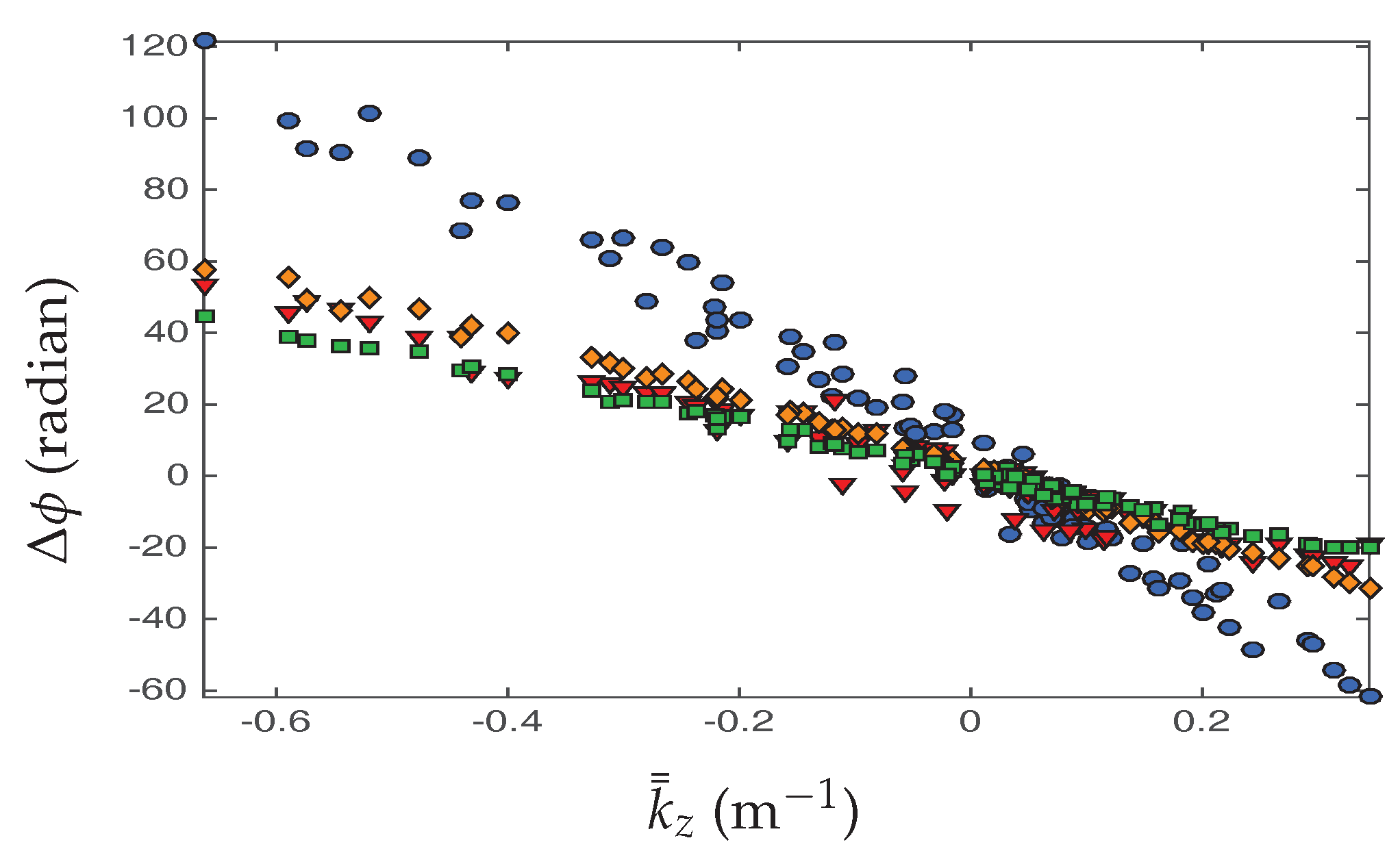
Figure 6.
Measured deformation given the number of days separating the acquisitions. (a) ![Remotesensing 09 01010 i002]() Eiffel Tower; (b)
Eiffel Tower; (b) ![Remotesensing 09 01010 i003]() Cristal Tower; (c)
Cristal Tower; (c) ![Remotesensing 09 01010 i004]() Keller Tower; (d)
Keller Tower; (d) ![Remotesensing 09 01010 i005]() Mirabeau Tower. The vertical dashed lines represent the years from the master image acquired the 24 January 2009.
Mirabeau Tower. The vertical dashed lines represent the years from the master image acquired the 24 January 2009.
Eiffel Tower; (b) Cristal Tower; (c) Keller Tower; (d) Mirabeau Tower. The vertical dashed lines represent the years from the master image acquired the 24 January 2009.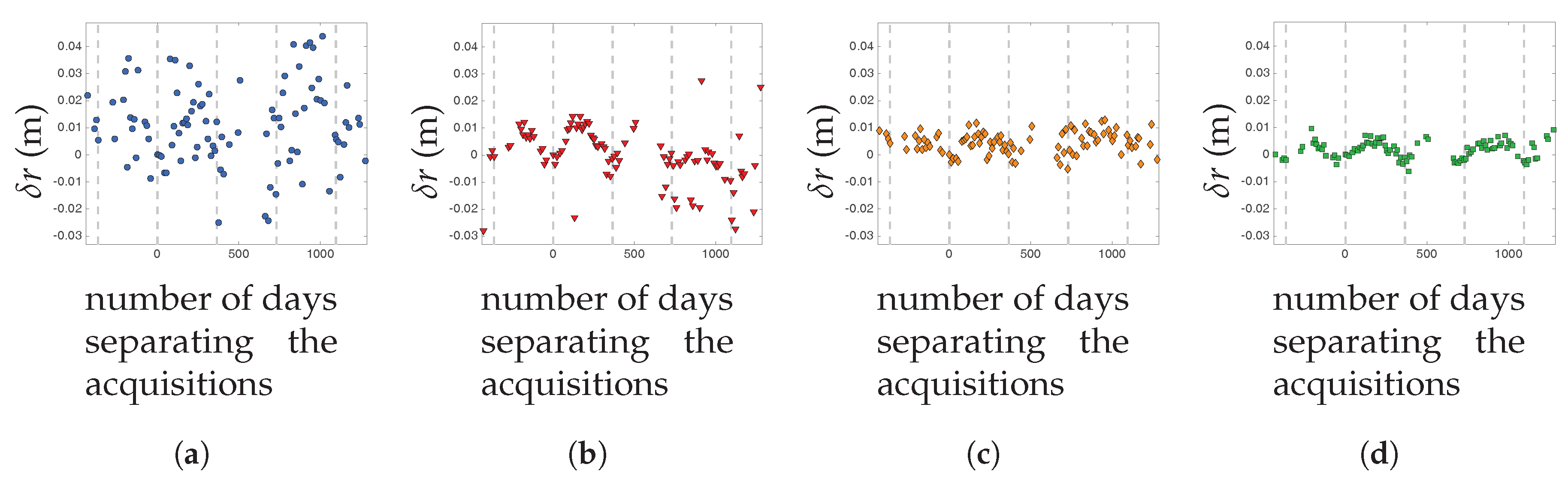
Figure 7.
Comparison between linear deformation measured by DInSAR ant the linear deformation measured by the optical strands installed on the Eiffel Tower by OSMOS. (a) Optical strand on the Eiffel Tower ©OSMOS (b) ![Remotesensing 09 01010 i002]() Lineic DInSAR deformation estimated for the Eiffel Tower — Minimal and Maximal lineic deformation measured by optical strands.
Lineic DInSAR deformation estimated for the Eiffel Tower — Minimal and Maximal lineic deformation measured by optical strands.
Lineic DInSAR deformation estimated for the Eiffel Tower — Minimal and Maximal lineic deformation measured by optical strands.
Figure 8.
(a) Polarimetric image in the Pauli basis; (b) interferometric image on the right in the HSV color space.
Figure 8.
(a) Polarimetric image in the Pauli basis; (b) interferometric image on the right in the HSV color space.
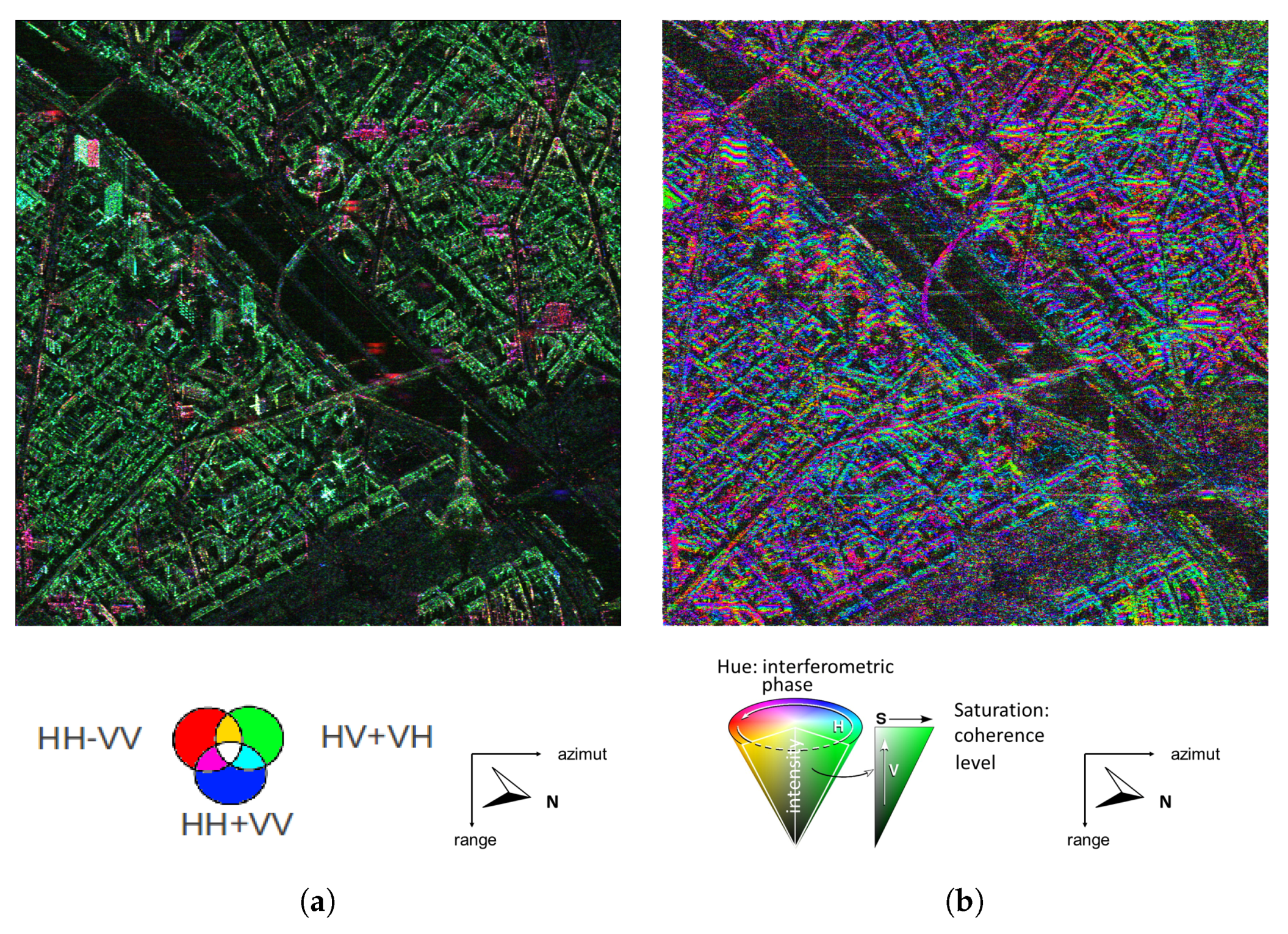
Figure 9.
Coherence optimization.

Figure 10.
Impact of the coherence optimization and optimum mechanisms (a) Interferometric coherence level in HH; (b) Interferometric level in optimal basis; (c) Colored composition where colors code the component magnitudes of the optimal mechanism.
Figure 10.
Impact of the coherence optimization and optimum mechanisms (a) Interferometric coherence level in HH; (b) Interferometric level in optimal basis; (c) Colored composition where colors code the component magnitudes of the optimal mechanism.

Figure 11.
The buildings analyzed using a dedicated 3D modeling (a) The ground Truth with the buildings as seens as the sensor; (b) The Ground Truth with the far side of the buildings; (c) Polarimetric images of the considered buildings.
Figure 11.
The buildings analyzed using a dedicated 3D modeling (a) The ground Truth with the buildings as seens as the sensor; (b) The Ground Truth with the far side of the buildings; (c) Polarimetric images of the considered buildings.
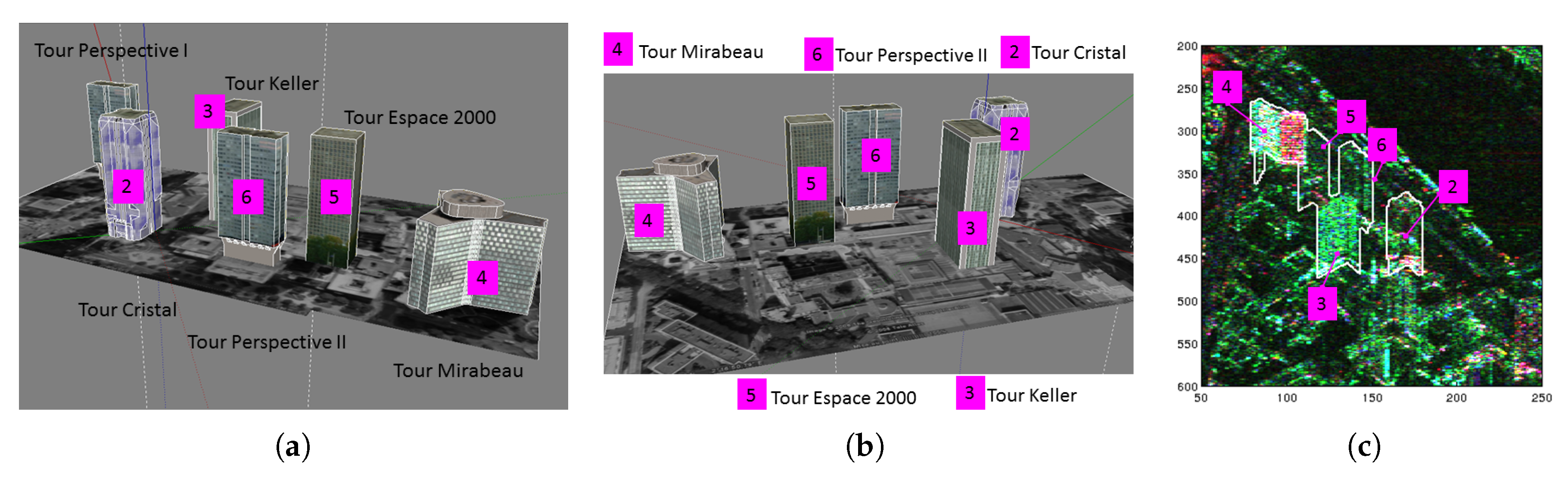
Figure 12.
Geometrical notation for computing the relation between azimuth orientation and polarimetric orientation.
Figure 12.
Geometrical notation for computing the relation between azimuth orientation and polarimetric orientation.

Figure 13.
Link between azimuth angle and polarimetric orientation angle for an horizontal vector and several incidence angles.
Figure 13.
Link between azimuth angle and polarimetric orientation angle for an horizontal vector and several incidence angles.
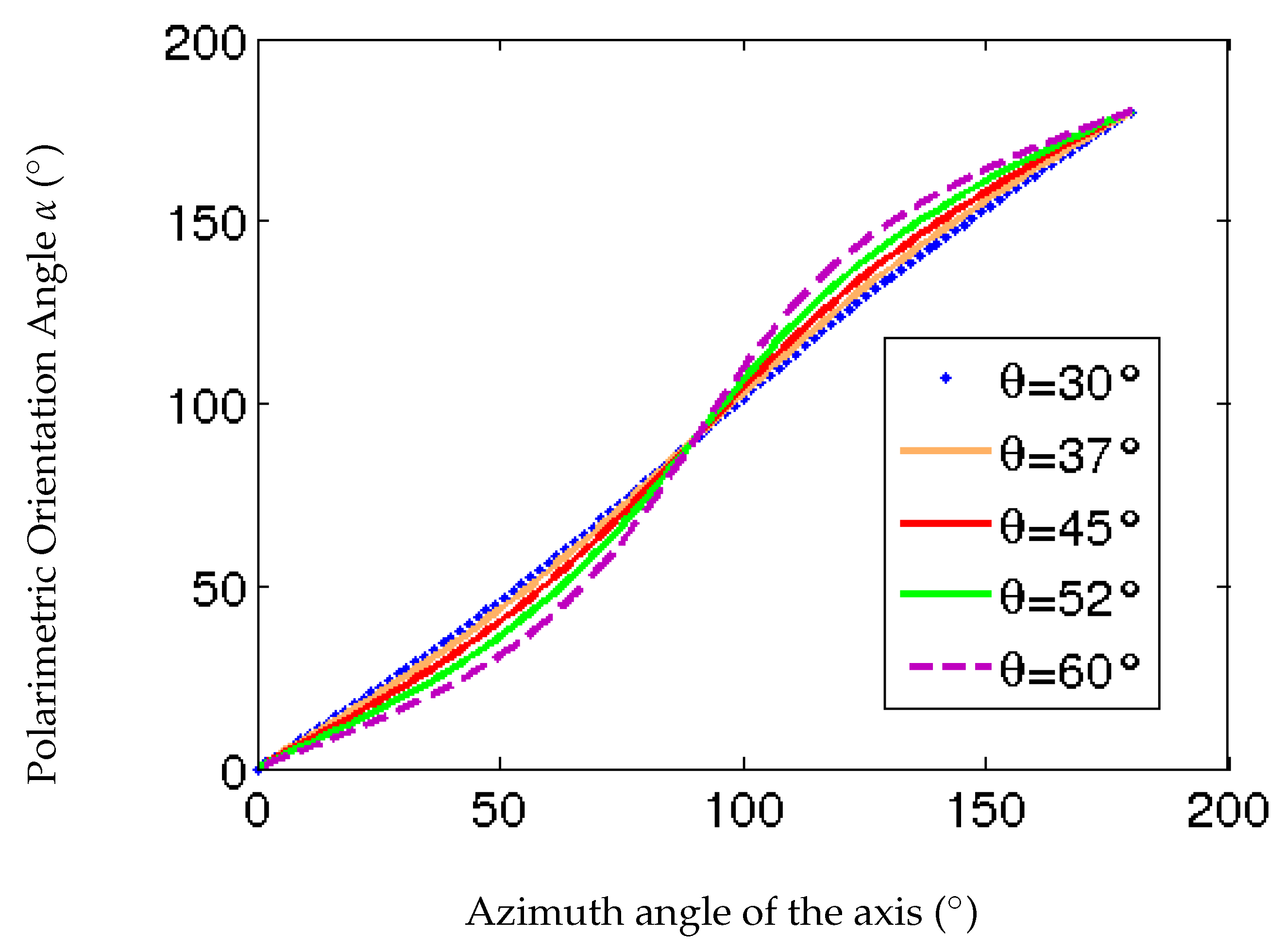
Figure 14.
Results of estimation of polarimetric orientation for the Mirabeau tower.

Figure 15.
Images of the buildings and detail of its facade, orientaion of the facade from the ground truth and results of estimation of polarimetric orientation. (a) Keller Tower (b) Espace 2000 Tower.
Figure 15.
Images of the buildings and detail of its facade, orientaion of the facade from the ground truth and results of estimation of polarimetric orientation. (a) Keller Tower (b) Espace 2000 Tower.
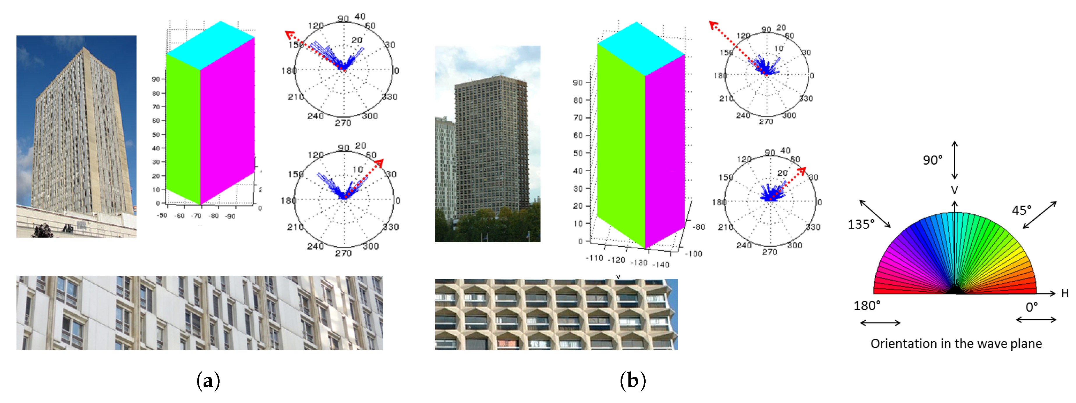
Figure 16.
Images of the buildings and detail of its facade, orientation of the facade from the ground truth and results of estimation of polarimetric orientation. (a) Cristal Tower (b) Perspective II Tower.
Figure 16.
Images of the buildings and detail of its facade, orientation of the facade from the ground truth and results of estimation of polarimetric orientation. (a) Cristal Tower (b) Perspective II Tower.
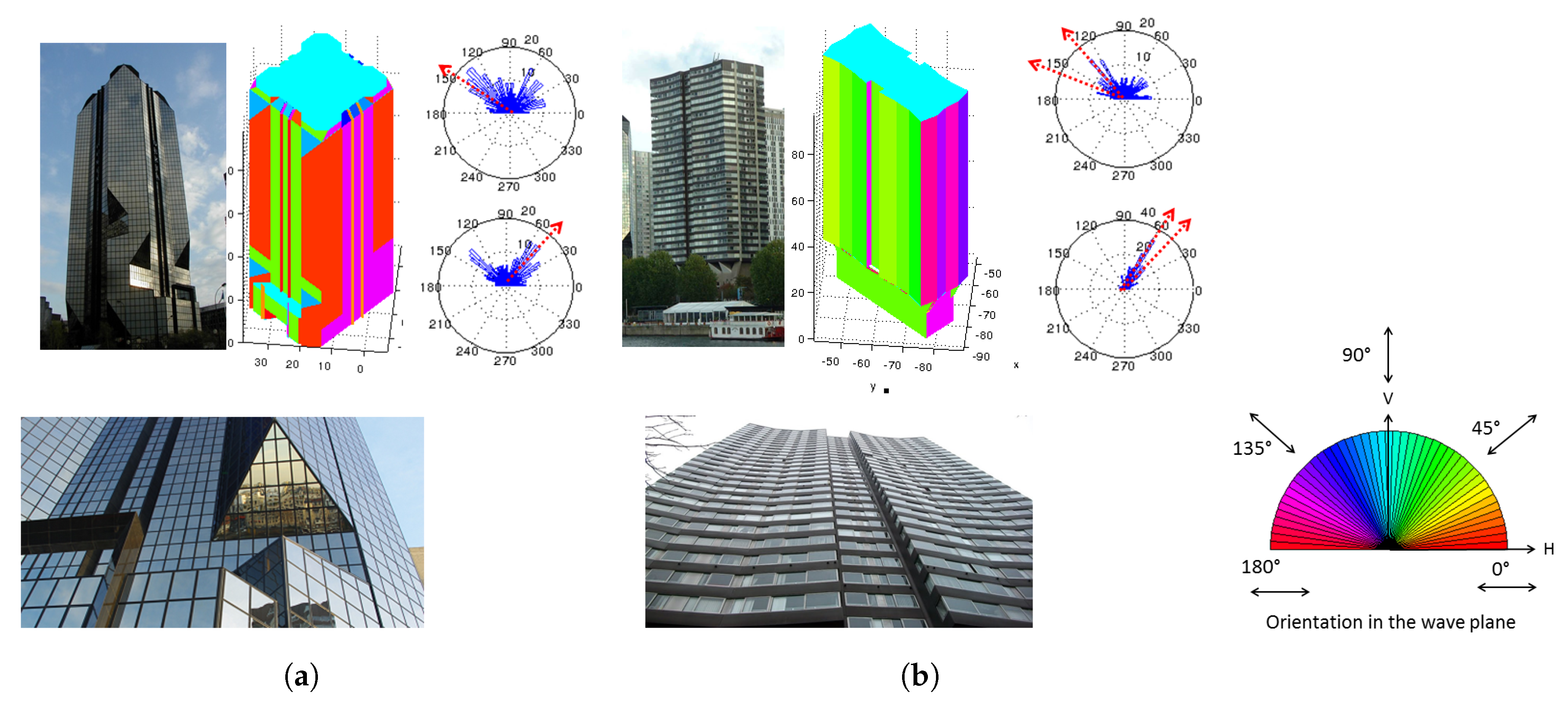
Figure 17.
Results of estimation of polarimetric orientation for the Tour Eiffel, compared with orientations of main beams, for stable orientations.
Figure 17.
Results of estimation of polarimetric orientation for the Tour Eiffel, compared with orientations of main beams, for stable orientations.

Figure 18.
Difference of (a) diattenuation and (b) retardance for the five different buildings.

Table 1.
Acquisition parameters of the TerraSAR-X temporal stack.
| Acquisition Parameters | Specifications |
|---|---|
| Satellite altitude | 514 km |
| Wavelength | 0.031 m |
| Look angle | 34.69 |
| Satellite-Earth distance R | 625 km |
| Ground-pixel size (azimuth and range) | = 0.87 m and = 0.71 m |
| Ground resolution (azimuth and range) | = 0.91 m and = 0.79 m |
| Slant range pixel size | 0.455 m |
| Acquisition time | 17:34 UTC |
Table 2.
Characteristics of the six studied buildings.
| Tower | Height | Facade Material | Facade Structure | Shape | |
|---|---|---|---|---|---|
| 1. | Eiffel | 321 m | Iron beams | ||
| 2. | Cristal | 98 m | Glass | Slanted corner | Rectangular cuboid |
| 3. | Keller | 98 m | Reinforced concrete | Concrete panels and windows | Rectangular cuboid |
| 4. | Mirabeau | 70 m | Reinforced concrete | Metallic window frame | Tripode |
| 5. | Espace 2000 | 98 m | Reinforced concrete | Small balconies | Rectangular cuboid |
| 6. | Perspective II | 94 m | Reinforced concrete | Concrete panels and windows | Butterfly-shape footprint |
Table 3.
Reference height, height measured by linear regression over the temporal stack and coefficient of determination of the regression.
Table 3.
Reference height, height measured by linear regression over the temporal stack and coefficient of determination of the regression.
| Eiffel Tower | Cristal Tower | Keller Tower | Mirabeau Tower | |
|---|---|---|---|---|
| h reference | 177.1 | 85.2 | 89.1 | 68.1 |
| h regression | 176.7 | 81.1 | 92.0 | 67.7 |
| 0.98 | 0.95 | 0.99 | 0.99 |
Table 4.
Normalized correlation with the deformation
| Eiffel Tower | −0.30 | 0.52 | −0.09 | −0.06 |
| Cristal Tower | −0.35 | 0.53 | 0.01 | −0.00 |
| Keller Tower | −0.27 | 0.48 | 0.02 | −0.15 |
| Mirabeau Tower | −0.73 | 0.81 | 0.53 | 0.08 |
© 2017 by the authors. Licensee MDPI, Basel, Switzerland. This article is an open access article distributed under the terms and conditions of the Creative Commons Attribution (CC BY) license (http://creativecommons.org/licenses/by/4.0/).
Share and Cite
MDPI and ACS Style
Weissgerber, F.; Colin-Koeniguer, E.; Nicolas, J.-M.; Trouvé, N. 3D Monitoring of Buildings Using TerraSAR-X InSAR, DInSAR and PolSAR Capacities. Remote Sens. 2017, 9, 1010. https://doi.org/10.3390/rs9101010
AMA Style
Weissgerber F, Colin-Koeniguer E, Nicolas J-M, Trouvé N. 3D Monitoring of Buildings Using TerraSAR-X InSAR, DInSAR and PolSAR Capacities. Remote Sensing. 2017; 9(10):1010. https://doi.org/10.3390/rs9101010
Chicago/Turabian StyleWeissgerber, Flora, Elise Colin-Koeniguer, Jean-Marie Nicolas, and Nicolas Trouvé. 2017. "3D Monitoring of Buildings Using TerraSAR-X InSAR, DInSAR and PolSAR Capacities" Remote Sensing 9, no. 10: 1010. https://doi.org/10.3390/rs9101010
Note that from the first issue of 2016, this journal uses article numbers instead of page numbers. See further details here.