Dimension Reduction of Multi-Spectral Satellite Image Time Series to Improve Deforestation Monitoring

Abstract

In recent years, sequential tests for detecting structural changes in time series have been adapted for deforestation monitoring using satellite data. The input time series of such sequential tests is typically a vegetation index (e.g., NDVI), which uses two or three bands and ignores all other bands. Being limited to a vegetation index will not benefit from the richer spectral information provided by newly launched satellites and will bring two bottle-necks for deforestation monitoring. Firstly, it is hard to select a suitable vegetation index a priori. Secondly, a single vegetation index is typically affected by seasonal signals, noise and other natural dynamics, which decrease its power for deforestation detection. A novel multispectral time series change monitoring method that combines dimension reduction methods with a sequential hypothesis test is proposed to address these limitations. For each location, the proposed method automatically chooses a “suitable” index for deforestation monitoring. To demonstrate our approach, we implemented it in two study areas: a dry tropical forest in Bolivia (time series length: 444) with strong seasonality and a moist tropical forest in Brazil (time series length: 225) with almost no seasonality. Our method significantly improves accuracy in the presence of strong seasonality, in particular the temporal lag between disturbance and its detection.

1. Introduction

Monitoring deforestation using satellite image time series has become an important component of forest management in recent years. Methods for monitoring deforestation from image time series in an automatic manner [1,2,3,4] were developed mainly based on a Monitoring of Empirical Fluctuation Process (MEFP) framework [5]. The MEFP framework consists of sequential hypothesis tests such as Cumulative Sum (CUSUM [6,7]) and Moving Cumulative Sum (MOSUM [8,9]) tests to monitor structural change. The MOSUM test is applied in a window moving over a time series and has been shown to be able to detect change more accurately than the CUSUM test [8,10]. The CUSUM or MOSUM test cumulatively aggregate the residuals of a linear model fitting to a time series to test the stability of the parameter estimates. A structural change is detected if newly-acquired observations deviate significantly from a model established on a stable time series. A time series thus is divided into two periods, a historical period consisting of stable time series and a monitoring period consisting of new observations. The observations in the historical period are called historical observations [11]. The input of the deforestation monitoring methods is typically a vegetation index, which is a spectral transformation of two or more spectral bands derived from satellite image scenes. Commonly-used vegetation indices for deforestation detection include NDVI (Normalized Difference Vegetation Index; [12]), NDMI (Normalized Difference Moisture Index; [13]), EVI (Enhanced Vegetation Index; [14,15]) and NBR (Normalized Burn Ratio; [16]). Furthermore, the TCT (Tasseled Cap Transformation; [17]) has been derived for MODIS [18] and Landsat sensors [19,20]. The TCT wetness component [21] was found to be related to forest structure [22] and has been applied to monitor deforestation [23]. Healey et al. [24] aggregated TCT components to contract the TCT brightness and other TCT components for change classification. These vegetation indices perform differently under different forest types, local climate and statistical models [25,26], thus causing the problem of selecting a proper vegetation index prior to deforestation monitoring.

Apart from vegetation index selection, a major challenge of using a single vegetation index is the separation of deforestation from multiple seasonality or climate effects. Seasonality can be modeled using time series spectral analysis (e.g., wavelet transform, Fourier analysis; [27,28]), time series modeling (e.g., autoregressive model; [27]) or smoothing methods (e.g., STL, the Seasonal-Trend decomposition procedure based on Loess; [29]). Hyndman and Khandakar [30] implemented exponential smoothing methods with a state-space modeling framework and ARIMA (Autoregressive Integrated Moving Average) models and applied an information criterion to automatically select models. The selected model can provide information about seasonality. Various forms of Fourier and wavelet transforms [31,32,33] were developed to flexibly model the seasonality of a time series. However, satellite imagery time series commonly contain missing data , which limits the application of these time series analysis tools. Verbesselt et al. [34] implemented a harmonic analysis model for time series breakpoint detection, which fits sine and cosine terms with a linear regression. This method is suitable for irregular time series and has been extensively applied to satellite image time series [1,3,4,23]. However, the model is limited to certain frequencies, as well as being restrained to using sine and cosine to describe seasonality. Therefore, it is difficult to construct a harmonic model to effectively capture the heterogeneity of forest ecosystems, the varying degree of forest cover change and complex climatic influences on the forest in a single vegetation index. Several studies attempt to better account for seasonality in the time series by normalizing the NDVI time series with the median of a spatial window [1], integrating spatial information into time series analysis with the SAR (spatial autoregressive) model [10] or introducing climate variables as independent variables in the regression model [4]. These studies utilized multi-dimensional information, but still constrain to using a single vegetation index.

The challenge associated with using a preselected vegetation index for deforestation detection can be addressed by using the whole spectral-temporal information in the satellite image time series. In this study, we propose to use PCA (Principle Component Analysis; [35]) directly on observations to automatically form an index for each location. PCA is a classical orthogonal dimension reduction method [36] to reduce the dimension from multi-spectral time series. PCA is known as a spectral decomposition (or transformation) method [37] in remote sensing. Its application ranges from noise removal in multi-spectral imagery to classification and land cover change detection [38,39,40,41]. In change detection, PCA has been most commonly applied to each image and detects change by comparing the PCA results of each image. In this study, we apply PCA to the time series of Landsat multi-spectral bands to improve the forest change monitoring capacity. We presume that PCA projects the multi-spectral time series to new axes, where the projected value of one axis measures forest presence, but is orthogonal to the axes that indicate brightness, seasonality and noise. The observations that are considered to be stable could be used to find such a dimension. The projected value in this axis forms the new index with reduced seasonality in its time series. We refer to the new index as SRI (Seasonality Reduced Index). Once the new index is formed, the MEFP is used to sequentially detect structural change in the time series. Our hypothesis test is that sequential test (e.g., [9]) on an index free from seasonality effects is more sensitive to change than a traditional index like NDVI, thus leading to accurate and timely detection of forest disturbances. We compared our method to the conventional vegetation indices and TCT components using Landsat TM and ETM+ data.

2. Study Area

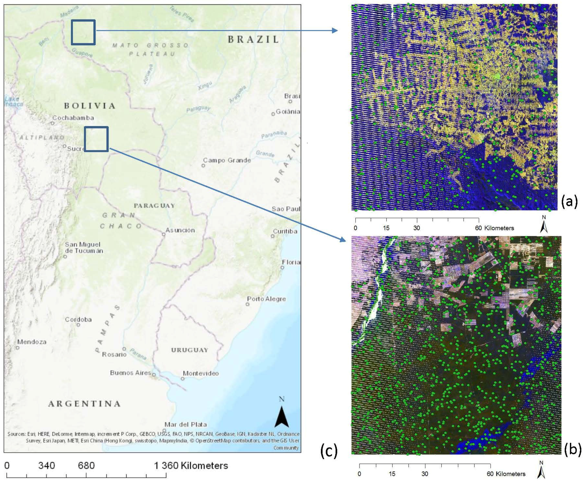
We evaluate our method at two study sites (Figure 1). One site is a dry tropical forest in the south east of Santa Cruz de la Sierra, Bolivia, South America (18.49${}^{\circ }$ S, 62.36${}^{\circ }$ W, $10,000$ km${}^2$), and the other is a moist tropical forest in the west of Ariquemes, Rondonia State, Brazil (centered at: 10.30${}^{\circ }$ S, 64.05${}^{\circ }$ W, $10,000$ km${}^2$). The Bolivian site is characterized by a dry season for several months of the year, and its forest is dominantly deciduous with strong seasonality. In contrast, the forest at the Brazilian site is evergreen and has almost no seasonality. A more detailed description of these two study sites can be found in Hamunyela et al. [1].

We used surface reflectance of all available terrain corrected (L1T) Landsat images (Thematic Mapper (TM) and Enhanced Thematic Mapper Plus (ETM+)), spanning from 1984–2014. A total of 444 images was available at the Bolivian site, and 225 images were available at the Brazilian site. We masked the pixels containing clouds and cloud shadows using an Fmask (Function of mask; [42]) as missing. The surface reflectance of the original L1T product is scaled by 10,000 [43]. The valid spectral reflectance range is therefore 1–10,000 [43]. The pixels with spectral reflectance outside this range are filtered out and considered missing. For each band, we removed extreme surface reflectance values from the time series using the method proposed by Hamunyela et al. [44]. The surface reflectances at time t that were less than 1% of both the reflectance at time $t-1$ and $t+1$ were considered as low extreme values and were therefore replaced by the mean of observations at time $t-1$ and time $t+1$.

3. Methods

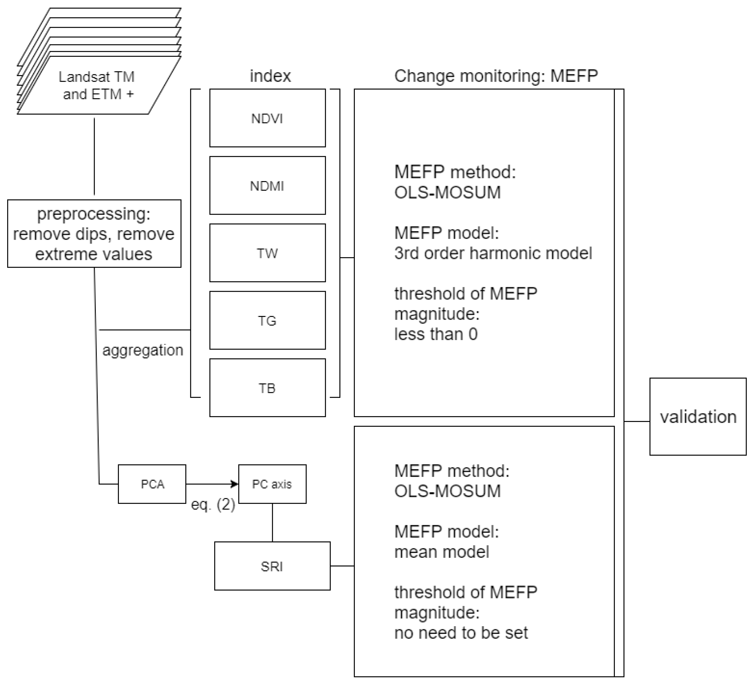
We propose a multispectral time series change monitoring method that combines PCA with sequential hypothesis tests to improve the detection of deforestation events. Section 3.1 explains the PCA. In this study, we used 6 (Bands 1–5 and 7) spectral bands of Landsat TM and ETM+ data; the PCA thus projects data to 6 PC axes. To fit into the univariate sequential test, at each pixel, a single PC axis needs to be selected. The proposed method uses a criterion to select a PC axis that is sensitive to the deforestation monitoring. The forming of the criterion and SRI is explained in Section 3.2. Once the SRI is derived, the MEFP framework is applied to SRI time series to detect deforestation events. The MEFP and how the SRI is monitored are described in Section 3.3. The seasonality assessment is described in Section 3.4. The comparison between SRI and the conventional vegetation indices is described in Section 3.5. We used a training dataset to explore the pattern of PC loadings and form the criterion and a separate testing dataset to validate the developed method.

3.1. PCA

Given a matrix X that contains n variables in its columns, PCA finds a projection matrix A of rank $q\le n$, so that the rotated data matrix $Y=XA$ is orthogonal, under the constraint that A is an orthogonal projector (i.e., $A^{\prime }A=I$). A can be found by eigenvalue decomposition of the covariance matrix of X (${\Sigma }_X$). Assuming X and Y are column centered, i.e., the mean of each variable (column) is subtracted from each observation, the covariance matrix of Y,

$$\begin{array}{cc}\hfill {\Sigma }_Y& =E\left(Y^{\prime }Y\right)\hfill \\ & =E\left(A^{\prime }{X}^{\prime }XA\right)\hfill \\ & =A^{\prime }{\Sigma }_{X}A\hfill \end{array}$$

(1)

is diagonal, and by convention, its variance ${\lambda }_1,\dots ,{\lambda }_n$ is arranged in descending order. The columns of A are the eigenvectors of ${\Sigma }_X$ and ${\lambda }_1,\dots ,{\lambda }_n$ the corresponding eigenvalues. The new variables (columns) in Y are the PC scores. We will call the eigenvectors the PC axes. We apply the PCA on the time series of Landsat spectral Bands 1–5 and 7 (for convenience, numbered as $j=1,\dots ,6$), at each pixel. Thus, at each pixel, $X={\left[\begin{array}{c}{X}_{ij}\end{array}\right]}_{(m\times 6)}$ contains the surface reflectance at times $i=1,\dots ,m$ for spectral bands $j=1,\dots ,6$, with m the length of a time series. The matrix A includes 6 columns, $a_i=\{a_{1,i},\dots ,a_{6,i}\}$ with the loadings for PC axis i; $a_{j,i}$ reveal how spectral band j relates to PC axis i. X is normalized (i.e., each spectral time series is centered to zero mean and standardized to unit variance), implying that we use the correlation matrix as the basis of the PCA.

3.2. Forming SRI

PCA is computed on the historical period of a multi-spectral time series array. The historical observations are projected to one of the PC axes and are used as the historical period for MEFP. The newly acquired data are projected to the same axis and are monitored by using the MEFP. The projected time series is:

$$y=X{a}_{\widehat{i}}$$

with $a_{\widehat{i}}$ the $\widehat{i}$-th column of A (i.e., the selected PC axis) and $X(m\times 6)$ the matrix of the original spectral time series after de-spiking.

To find the PC axis that is suitable for deforestation monitoring, we used an additional training dataset of 100 points sampled from non-deforested locations of each study site to explore the pattern of PC loadings. The data are organized as $X={\left[\begin{array}{c}{X}_{ij}\end{array}\right]}_{(N\times 6)}$, which contains surface reflectance at times $i=1,\dots ,N$ for spectral bands $j=1,\dots ,6$, now with N the sum of the lengths of all time series ($100\times 444=44,400$ for the Bolivian site and $100\times 225=25,500$ for the Brazilian site).

The first 3 PCs all together explain more than 90% of the correlation for both study sites. The first 4 PC loadings of the validation time series that contain no deforestation events are shown in Figure 2a for the Bolivian site and Figure 2b for the Brazilian site.

Based on the spectral reflectance of dry and green vegetation of different wavelength [45], we interpret the first PC (PC1, Figure 2) as the general brightness, the second PC (PC2) of the Bolivian site (Figure 2a) and the third PC (PC3) of the Brazilian site (Figure 2b) as the vegetation greenness fluctuation, which often contains seasonality that is affected by climate and can hinder the identification of deforestation. The PC3 of the Bolivian site (Figure 2a) and the PC2 of the Brazilian site (Figure 2b) indicates a contrast between visible and IR (near infrared and shortwave infrared) bands. As the IR bands are sensitive to water, the PC3 of Figure 2a and the PC2 of Figure 2b relate to the wetness. The seasonality effects and the general brightness explained by the other PCs are exempt from this PC. We thus hypothesize the PC that is related to the wetness (i.e., PC3 of Figure 2a and the PC2 of Figure 2b) to be suitable for deforestation monitoring.

Based on the PC loadings, a criterion is determined empirically to automatically select for each time series the PC axis that is hypothesized to be sensitive to deforestation. Based on the criterion, SRI is chosen as the PC axis i that maximizes contrast between visible bands and IR bands by:

$$\widehat{i}=\underset{i}{arg\; max}|(a_{i,1}+a_{i,2}+a_{i,3})-(a_{i,4}+a_{i,5}+a_{i,7})|$$

(2)

where $a_i$ indicates the i-th PC axis, and the $\widehat{i}$ indicates the PC axis that is chosen.

3.3. Monitoring Deforestation Using SRI

The proposed method is depicted in Figure 3. The MEFP is applied to the SRI once it is formed.

The MEFP considers the cumulative difference between the value of newly acquired data and the prediction of a model fitted to historical observations. The steps are as follows:

• The model is estimated on a stable historical period where the parameters are assumed to be stable.
• A fluctuation process is initialized and captures deviations from the model. Under the null hypothesis, the fluctuation process converges to a Gaussian stochastic process.
• For each incoming observation, the fluctuation process is updated. If the fluctuation process exceeds the threshold for the limiting Gaussian process, there is evidence that the structure of the time series has changed.

The historical period is assumed to be stable, i.e., it contains only forests, and no deforestation event has occurred during the historical period. A mean model is fitted to the SRI as the seasonality is assumed to be filtered out. Deforestation is declared if a structural change is detected in the SRI time series. We used the MOSUM-OLS (Ordinary Least Square) model of the MEFP [9] to detect structural changes in the SRI time series.

3.4. Seasonality Assessment

Our study hypothesizes that the seasonality is reduced in SRI. To test this hypothesis, we compared the seasonality between SRI and NDMI. The additional testing dataset of the Bolivian site from the forest stratum is used. We use the amount of variance that is explained in first-order harmonic model to quantify the annual seasonality of a time series. Firstly, a first-order harmonic model is fitted to a time series. Then, the coefficient of determination ($R^2$) of the fitted model is calculated to indicate the variance explained by the harmonic model.

3.5. Comparison of Different Indices

To determine how our method performs in comparison to the vegetation indices and the TCT components, we also detected deforestation from NDVI, NDMI, TCT Greenness (TG), TCT Brightness (TB) and TCT Wetness (TW) time series over the same period. The NDVI is calculated as $NDVI=(NIR-Red)/(NIR+Red)$. The NDMI is calculated as $NDMI=(NIR-SWIR)/(NIR+SWIR)$. The TCT indices are calculated using the bands’ weight given in Crist and Cicone [21] for Landsat TM 5 data and in Huang et al. [20] for Landsat ETM+ 7 data. Similar to SRI, we used the MOSUM-OLS (Ordinary Least Square) model to detect structural changes in the time series of vegetation indices and TCT components. Different from the SRI, we fitted the first-order harmonic model to the time series of vegetation indices and TCT components to account for seasonality effects. In addition, a magnitude of change, defined as the difference between the mean of the harmonic model fitted to the historical observations and the value at the change point, is required to be negative when a structural change is detected to declare deforestation. Figure 4 shows the procedure of our experiment comparing different indices.

4. Accuracy Assessment

Elaborate and reliable validation data for forest disturbances do not exist in many parts of the globe. As an alternative, here, we rely on the reference datasets (test dataset) acquired through visual interpretation of Landsat multispectral images to assess the accuracy of our analysis in space and time. To facilitate the collection of reference data, we first stratified each study area into two strata: forest and deforested. Forest and deforested areas were digitized manually from Landsat multispectral image time series. For the Bolivian site, we used 1136 reference sample pixels (deforested stratum = 103, forest stratum = 1033), whereas at the Brazilian site, we used 470 reference sample pixels (deforested stratum = 141, forest stratum = 329) to estimate the accuracy of our analysis. In addition to the test dataset, we used training sample pixels to explore the pattern of PC loadings, where 100 sample pixels were from forest stratum at each study site. All sample pixels where selected through stratified proportional random sampling. For the validation points from deforested stratum, we documented the date of deforestation by identifying the first image on which the deforestation event was visible. Those dates were subsequently used as surrogate dates for deforestation. It should be noted however that reference datasets acquired through visual interpretation of satellite images have limitations. For example, disturbed areas that are not visually visible from multispectral images might be wrongly classified as forest, thus resulting in underestimation of the area that has been disturbed. To minimize this problem, we complemented the interpretation of dense Landsat time series with visual interpretation of high resolution images from Google Earth.

We used an accuracy measure suggested in Pontius et al. [46], the figure of merit [47], as a measure to assess the overall results in space, so that an overly high overall accuracy caused by large amounts of unchanged pixels can be avoided. The figure of merit is defined as: $TP/(TP+FN+FP)$, where TP, FN and FPindicate True Positive, False Negative and False Positive, respectively. In addition, we calculated the producer’s accuracy and the user’s accuracy to assess if the errors are dominated by FNs or FPs. The user’s accuracy is calculated as $TP/(TP+FP)$ and the producer’s accuracy as $TP/(TP+FN)$. In some cases, the change is signaled earlier (early detection) than the real change. We counted such detection as an FP. 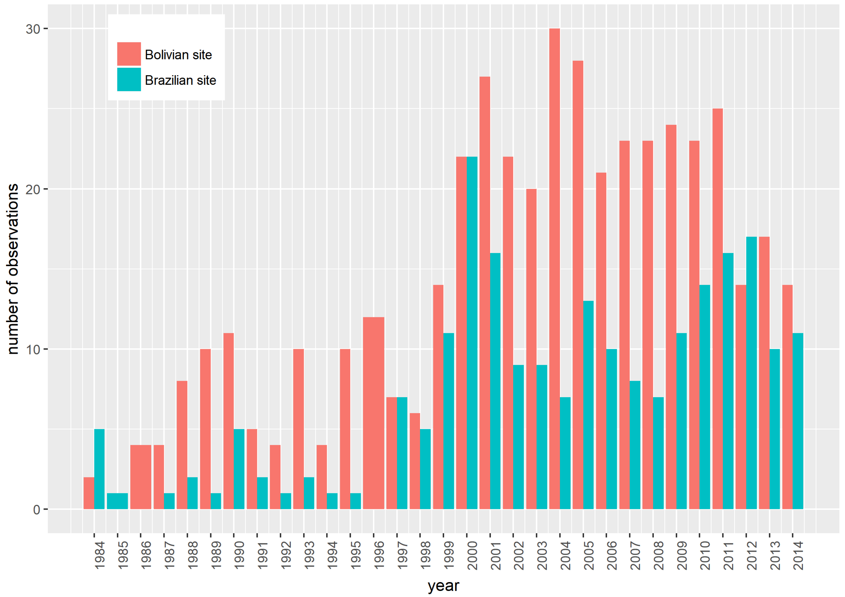To compare with other change monitoring studies, the overall accuracy ($(TP+TN)/(TP+FN+FP+TN)$) is computed. The temporal delay was calculated as the number of observations between the image in which MEFP detected change and the image in which the deforestation event was first visible as per reference data. A median temporal delay was calculated from validation points where deforestation events were detected correctly. Because of the irregularity of Landsat data, using the number of observations is a more straightforward measure compared to using the difference in time. The number of available Landsat TM and ETM+ images of each year from 1984–2014 is shown in Figure 5

5. Results

The deforestation detection results are reported in

Table 1. Figure Of Merit (FOM, %), Producer’s Accuracy (PA, %), User’s Accuracy (UA, %), Overall Accuracy (OA, %) and Temporal Delay (TD, observation) at the Bolivian site. A mean model is used in the MEFP for the method introduced here (SRI), and a first-order harmonic model is used for the other indices.

	FOM	PA	UA	OA	TD
SRI	39.4	87.5	41.8	88.6	6
NDMI	19.9	81.3	20.8	73.8	19
NDVI	21.5	54.6	26.2	83	24
TB	15.8	18.4	52.8	91.1	41
TG	21.5	79.6	22.7	74.9	17
TW	22	99	22	70.3	5

and

Table 2. FOM (%), PA (%), UA (%), OA (%) and (observation) at the Brazilian site. A mean model is used in the MEFP for the method introduced here (SRI), and a first-order harmonic model is used for the other indices.

	FOM	PA	UA	OA	TD
SRI	17.7	64.6	19.6	47.4	11
NDMI	22.4	62.5	25.9	59.6	17
NDVI	18.4	44.3	23.9	63.2	16
TB	9.5	13.9	23	65.5	27
TG	21.1	54.9	25.6	55.5	24
TW	20.3	87.1	20.9	38.1	30

for each study area. At the Bolivian site, the accuracy measures indicate that using the SRI outperforms other vegetation indices (i.e., TW, TG, TB, NDMI and NDVI). The SRI and the TW improved temporal delay greatly compared to the NDVI, NDMI, TG and TB. However, the TW achieved a relatively low user’s accuracy. Both NDVI and NDMI detected change with long temporal lags.

The results of the Brazilian site show a low figure of merit achieved in general. The SRI still achieved the shortest temporal lag, but less significant than in the Bolivian case. Contrary to the Bolivian case, the TW resulted in the longest temporal lags among other indices. The NDMI and the SRI achieved relatively high producer’s accuracy. This may indicate that the NDMI and the SRI are more noise-resistant.

In both cases, NDMI shows a higher producer’s accuracy compared to NDVI. In addition, the relatively low user’s accuracy compared to the producer’s accuracy for all the indices indicates that the FPs dominate the total error.

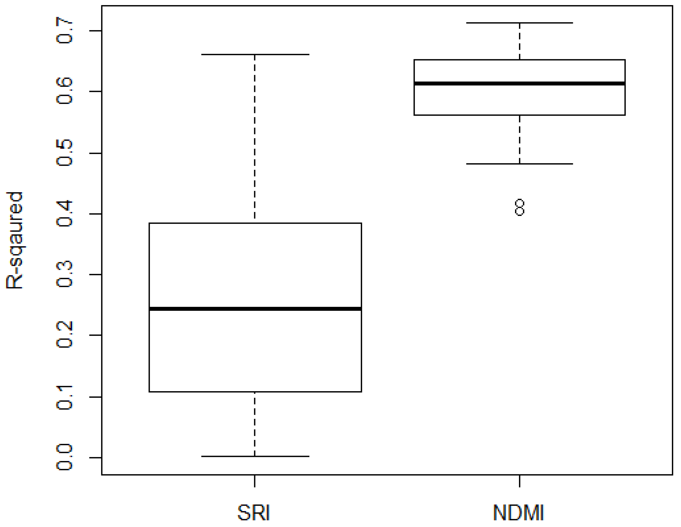
Comparison of Seasonality in SRI and NDMI

We assess the seasonality of SRI and compare it with the seasonality in the corresponding NDMI, which obtained slightly better results comparing to NDVI in our experiment. The result is summarized in the boxplot (Figure 6), which indicates more variance is explained by harmonic terms in NDMI (median: 0.61) than in SRI (median: 0.24). This confirms our hypothesis that the SRI contains reduced seasonality.

6. Discussion

We applied PCA to multispectral time series to substitute the use of a single vegetation index, which by filtering the seasonality of a time series improves the detection of forest disturbances from satellite image time series.

The developed method was tested on a dry forest with strong seasonality and on a moist forest with mild seasonality. The major contribution of this study is to go beyond using a pre-selected vegetation index and develop a data-driven method to extract information from all the optical spectral bands of each pixel. Considering the spatial heterogeneity of forests, our study is a step towards a fully-automatic deforestation monitoring system, which has an important implication for global-scale deforestation monitoring. In addition, our study shows transforming all the optical spectral bands may integrate more information and deal with the seasonality effects. At last, we provided a simple criterion (Equation (2)) to tackle the challenge that PC axes are only ordered by their eigenvalues.

The discussion begins with an explanation of the achieved accuracy by comparing example time series of all indices (Section 6.1). Then, we discuss the method of applying PCA to the entire time series (Section 6.2). Finally, the advantages, limitations and future works of the developed method are discussed (Section 6.3).

6.1. Indices Comparison

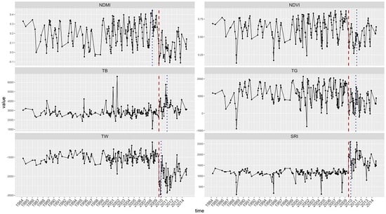
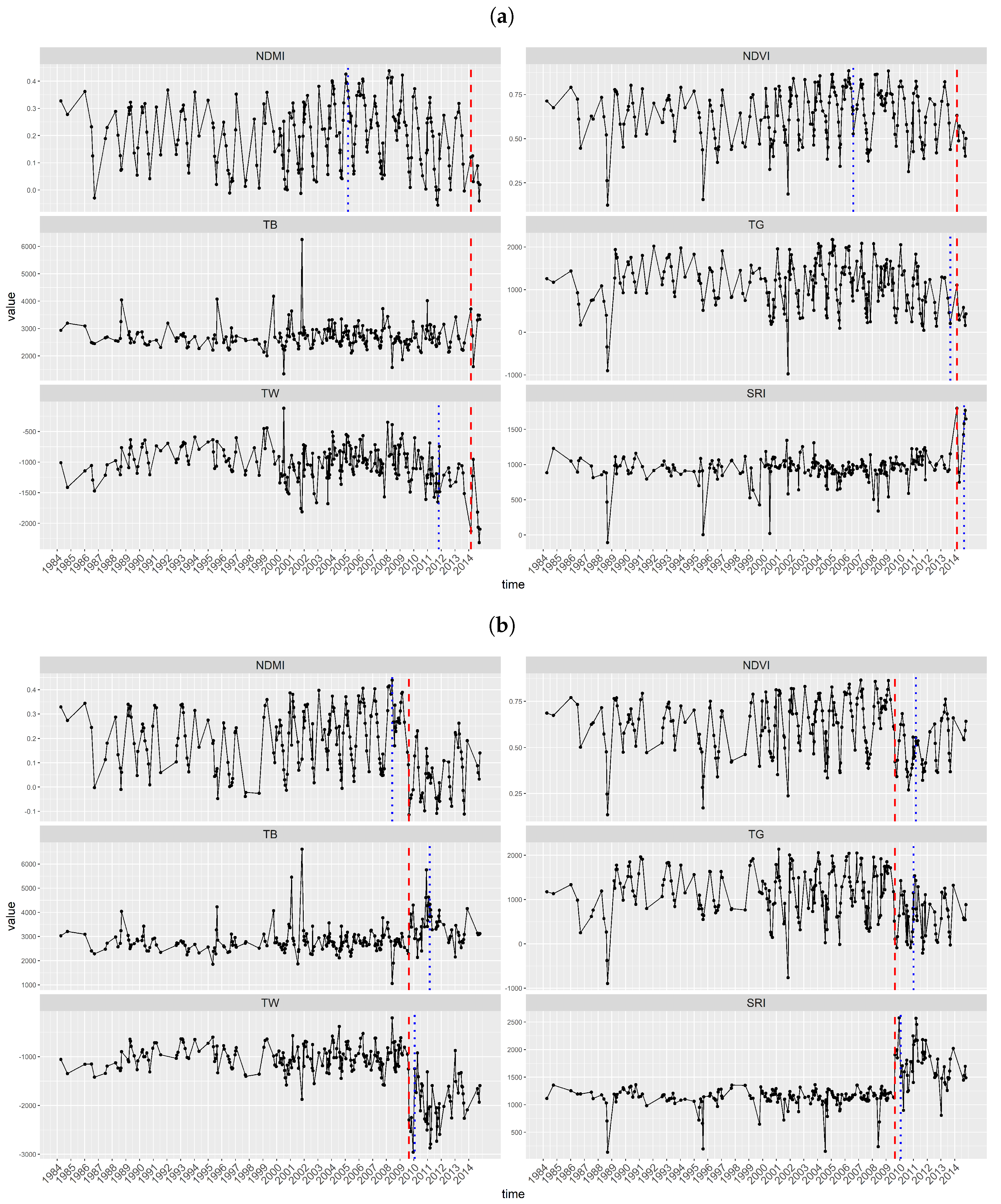
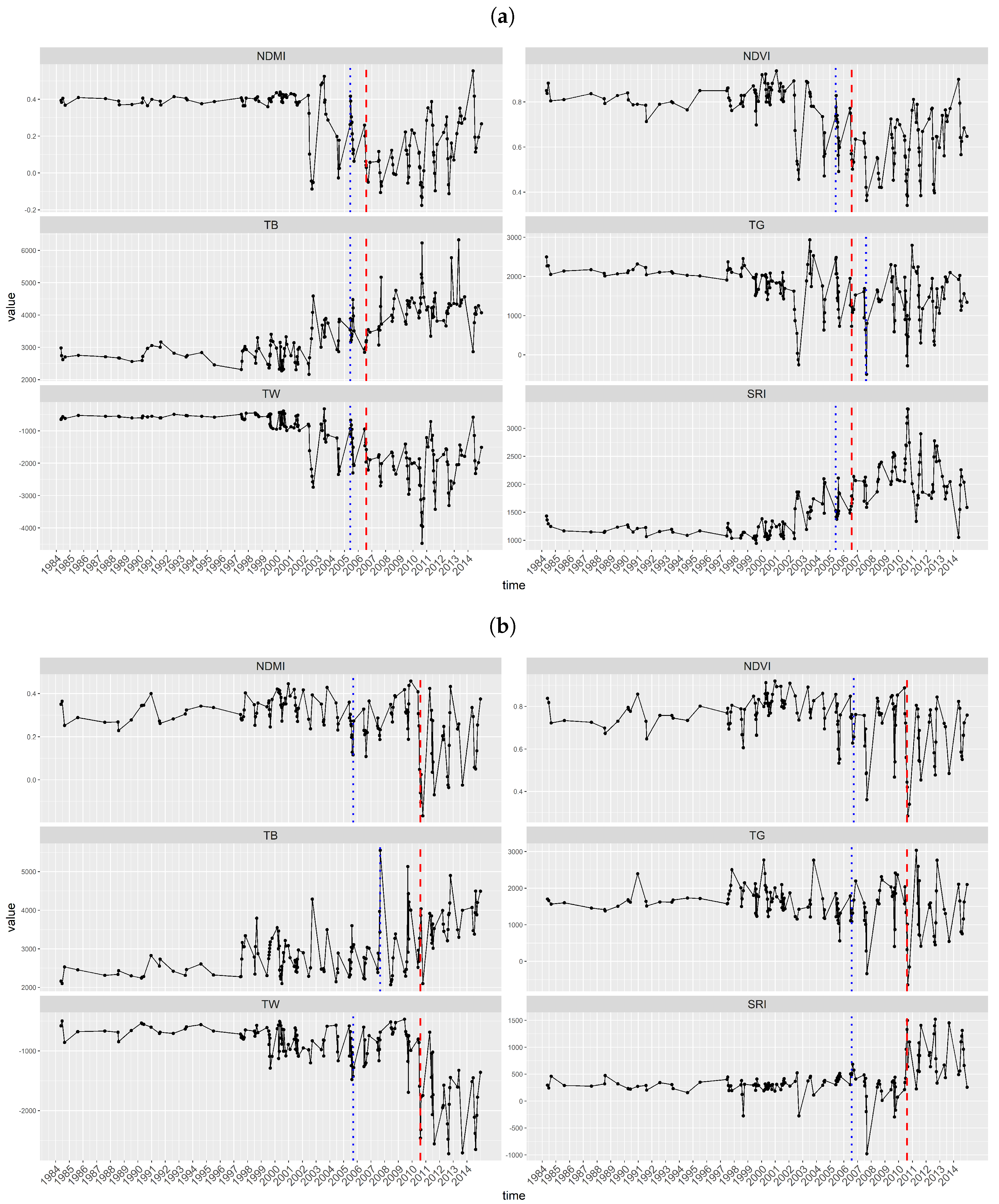
Our results indicate a significantly improved accuracy with the SRI at the Bolivian site (Figure 1) where the seasonality is strong. Compared to those from the Bolivian site, all the indices from the Brazilian site (Figure 2) received similarly inferior results in space, especially low user’s accuracy. To better understand the behavior of each index, we observed the time series of NDMI, NDVI, TG, TB, TW and SRI. For each study site, two examples are shown for illustration (Figure 7 and Figure 8).

Several factors could have led to the unsatisfactory results obtained for the Brazilian site. First, the time series are less dense than the Bolivian site. The deforestation information may have been missed especially under fast regrowth. Secondly, both randomly selected locations of the Brazilian site (Figure 8a,b) show early detection with every vegetation index. The early detection is likely caused by a severe drought that happened in 2005. When creating the validation dataset, the deforestation events are less obvious and harder to identify for the Brazilian site from the Landsat images due to a larger amount of low quality images and because deforestation events are typically smaller when compared to the Bolivian site. Figure 8a shows a drop of reflectance in 2002 for NDVI, NDMI, TG and TW. However, from the Landsat time series, not until 2005 could a deforestation event be identified. This resulted in early detection (FP) with all the indices at the location. To test if the FPs at the Brazilian site are due to early detection, we set the changes that were detected early as TPs in the validation process. Compared to the results when the early detected changes were set as FPs, the figures of merit obtained by SRI, NDVI, NDMI and TW are much higher (37.3%, 44.7%, 44.9% and 36%, respectively). This test indicates early detections as an important source of FPs, which are likely to be caused by the above factors.

At the Bolivian site, the NDVI and NDMI indices show seasonal dynamics, which can lead to false change detection as in Figure 7a, NDMI, NDVI, and Figure 7b, NDMI, as well as disguising the change signal, which then leads to late change detection as in Figure 7b, NDVI. The SRI shows less seasonality and a clear structural change close to the time of deforestation. At the Brazilian site (Figure 8), the NDMI and NDVI time series show almost no seasonality. With almost no seasonality, the change signal is likely to be pronounced in the signal of a vegetation index. This might be the reason that using the proposed method does not improve the spatial accuracy. The time series of TW is similar to the time series of SRI at 18.364${}^{\circ }$ S, 62.584${}^{\circ }$ W (Figure 7b), but it is different from the time series of SRI at 18.341${}^{\circ }$ S, 62.541${}^{\circ }$ W (Figure 7a). The reason is that the TCT was calibrated, and the weight is fixed for each component, while SRI is formed per pixel by selecting the PC component that is the most sensitive to deforestation (Equation (2)). The use of TW obtained similarly short temporal delay as SRI at the Bolivian site, but the longest temporal delay at the Brazilian site, which may indicate more steady performance of SRI. TW is subjected to vegetation type and other environmental factors; therefore, it may be less reliable for deforestation monitoring. This can be observed in the two examples (Figure 7) of the Bolivian site; a false positive is detected using the TW in Figure 7a TW, whereas the change is detected at an optimal time in Figure 7b TW.

6.2. Applying PCA to the Whole Time Series

Instead of applying PCA to a stable historical period only, PCA could be applied to the whole time series to account for change information from new observations, taking each recomputed PC score as the input to MEFP. If there is a change in the seasonality of newly acquired data, this information is analyzed in PCA. We have applied PCA to the whole time series and obtained very similar results to the SRI. The implementation and reproducible codes of this method can be found in the multibandsBFAST R package mentioned at the end of Section 1.

6.3. Advantages, Limitations and Future Studies

The complex seasonality in forests hinders an accurate automated deforestation monitoring process. Kennedy et al. [48] apply time series segmentation methods to annual data to avoid seasonality. A harmonic model may not be flexible enough to identify the seasonality and is not adaptable to heterogeneous forest cover types. Higher order harmonic models can cause over-fitting of sparse time series [3]. Dutrieux et al. [4] integrate a precipitation variable in the regression model of MEFP, which improved the overall accuracy, but did not completely remove the seasonality effects. This may be due to the complex interactions between climate and the forest system. We demonstrate here that by applying PCA to multiple spectral time series, the seasonality effects and noise could be reduced for change monitoring purposes. In our study, the SRI is related to the wetness; the wetness seasonality that is correlated to the vegetation greenness seasonality is also filtered out from the SRI.

Zhu and Woodcock [49] proposed a method that uses all the spectral bands of Landsat data. However, Zhu and Woodcock [49] analyzed each band independently and did not solve the aforementioned problem of seasonality effect. In addition, Zhu and Woodcock [49] detected change using a ratio of the differences between new observations and the predictions of a linear regression model estimated from historical records vs. the residuals of the linear regression model. Comparing to Zhu and Woodcock [49], the MEFP uses more information from the historical record and may be more stable and robust against noise. Moreover, the SRI reduces the multiple spectral bands into a single index and is computationally more feasible. The SRI is related to the TW component in our study cases. The TCT is also an orthogonal transformation. The difference is that the PCA forms the index based on the behavior of spectral bands time series, while the TCT components were derived by transforming preselected features of satellite scenes [21]. The forming of SRI is based on the spectral time series characteristics of the application area. For natural forest systems where the vegetation types are heterogeneous, the SRI is computed for each pixel time series, and the accuracy of the methods may be improved with higher spatial resolution data. In a homogeneous region, the PCA can be applied to one or a few sampled pixels to form the SRI for the whole region.

Spectral bands contain redundant information. PCA is able to extract non-redundant information without the need to choose wavelength bands. For example, though the blue band is highly correlated with the green and red bands and is known to contain much noise for forest study, the PCA result will not be negatively influenced. The dimensional reduction method is particularly useful as the difficulty of manually choosing a proper band combination increases with higher spectral resolution.

In addition to reduced seasonality effects and noise, SRI may reduce the influence from orbit drifting [50] and sensor degradation [51]. The long-term spectral band trends caused by the orbit drifting [50] may lead to weakening of the deforestation signal. Further investigations are needed to quantify the effects of orbit drifting and sensor degradation on SRI and to adjust the proposed method to reduce the orbit drifting and sensor degradation effects to the minimum.

The method presented in Section 2 has the advantage that it is easy to understand and to apply. We did not evaluate the particular component selection criterion (Equation (2)) or the decision to use principle components in general. The coefficients of Equation (2) (now: $(1,1,1,-1,-1,-1)$) could be optimized to ensure the PC axis that is sensitive to deforestation will be correctly selected when other remote sensing products (e.g., Sentinel 2) are used. Another alternative involves dropping principle components altogether in favor of linear combinations of the bands that are directly optimized to predict forest change. The current study should be seen as a first step in this direction; the computational challenges that are involved in both of these optimizations prohibited their implementation.

We form the SRI based on the hypothesis that by orthogonally decomposing data, the seasonality contained in other PC components can be filtered out. Besides the seasonality analysis in the manuscript, this hypothesis is further supported with a seasonality analysis of PC components; the method and results are described in the Supplementary Material “Seasonality Analysis”. The potential of the proposed method with the increased number of spectral bands needs to be studied. For example, Sentinel-2 has 13 spectral bands, and the PCA may transform the data in a direction that is more related to some forest features and sensitive to deforestation. With the SRI, the time series that is needed for the historical period can be shorter than the conventional vegetation indices as the modeling of the seasonality (e.g., annual cyclic) of a time series is unnecessary. In addition, this approach may be applied to data from different sensors to further improve the spatial and temporal accuracy in deforestation detection. Furthermore, the proposed method can be extended for the PC to point to meaningful directions: (1) the PCA input matrix may be formed with different bands normalizations and spatial information; (2) the kernel PCA [52] may be used to find more interesting information from higher dimensions.

An R package multibandsBFAST that contains all the functions and data that were used in this study was created. All the results and figures in this paper are reproducible using the scripts found at https://github.com/mengluchu/multibandsBFAST.

7. Conclusions

This paper introduces the Seasonality Reduced Index (SRI) that combines multispectral bands and reduces the seasonality in the input time series of change monitoring models. A new approach is presented here to show how PCA can be used to integrate pixel time series of multispectral bands to improve pixel-based deforestation monitoring. The developed approach is evaluated in two study areas, a dry and a moist forest, and it was compared to widely-used vegetation indices. The SRI outperforms the NDVI, NDWI and TCT components at the Bolivian site, where strong seasonality dominates the forest dynamics. The TW shares the same origin as the SRI, but is less flexible and produced less favorable and reliable results. At the Brazilian site, the SRI yielded slightly worse spatial accuracy compared to NDVI and NDMI, but was able to detect deforestation events early; the use of TW led to a long temporal delay. Our study is a first step toward utilizing multispectral time series to overcome the problems of single vegetation indices, which ignore most spectral information. Further work is required to investigate the application of PCA to larger sets of spectral bands, optimize the numeric criterion to automatically select the PC, integrate spatial and other thematic information and use PCA extensions or other alternatives to PCA to investigate the full potential of dimension reduction methods in change monitoring.