A Modified Multi-Source Parallel Model for Estimating Urban Surface Evapotranspiration Based on ASTER Thermal Infrared Data

 ,
,  ,
,
Abstract
:
1. Introduction
- (i)
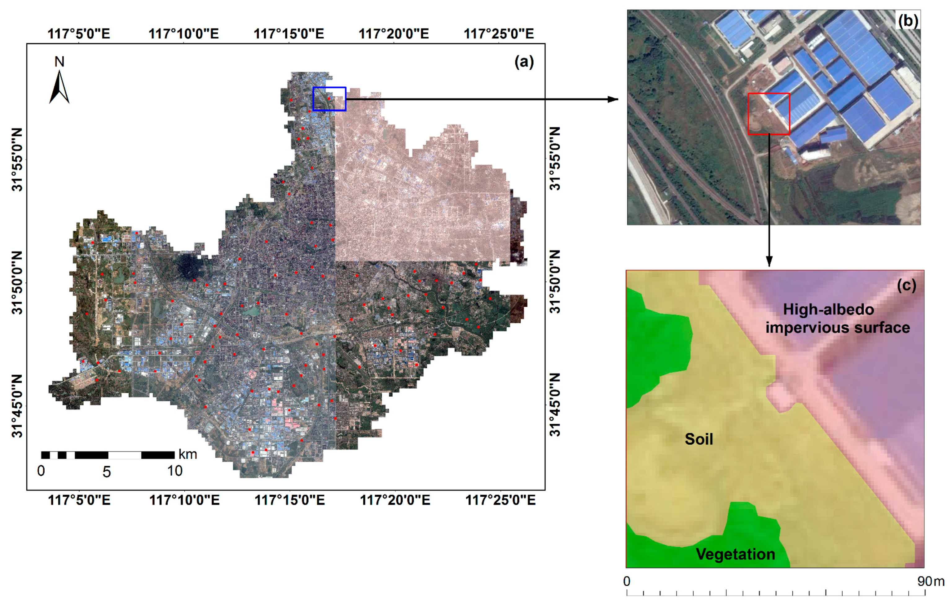
- Characterizing spectrally heterogeneous urban impervious surfaces with two spectral endmembers (high- and low-albedo);
- (ii)
- Revising the methods of deriving roughness length for each land surface component;
- (iii)
- Recalculating the component net radiant flux with a full consideration of the fraction and the characteristic of each land surface component.
2. Study Area and Data
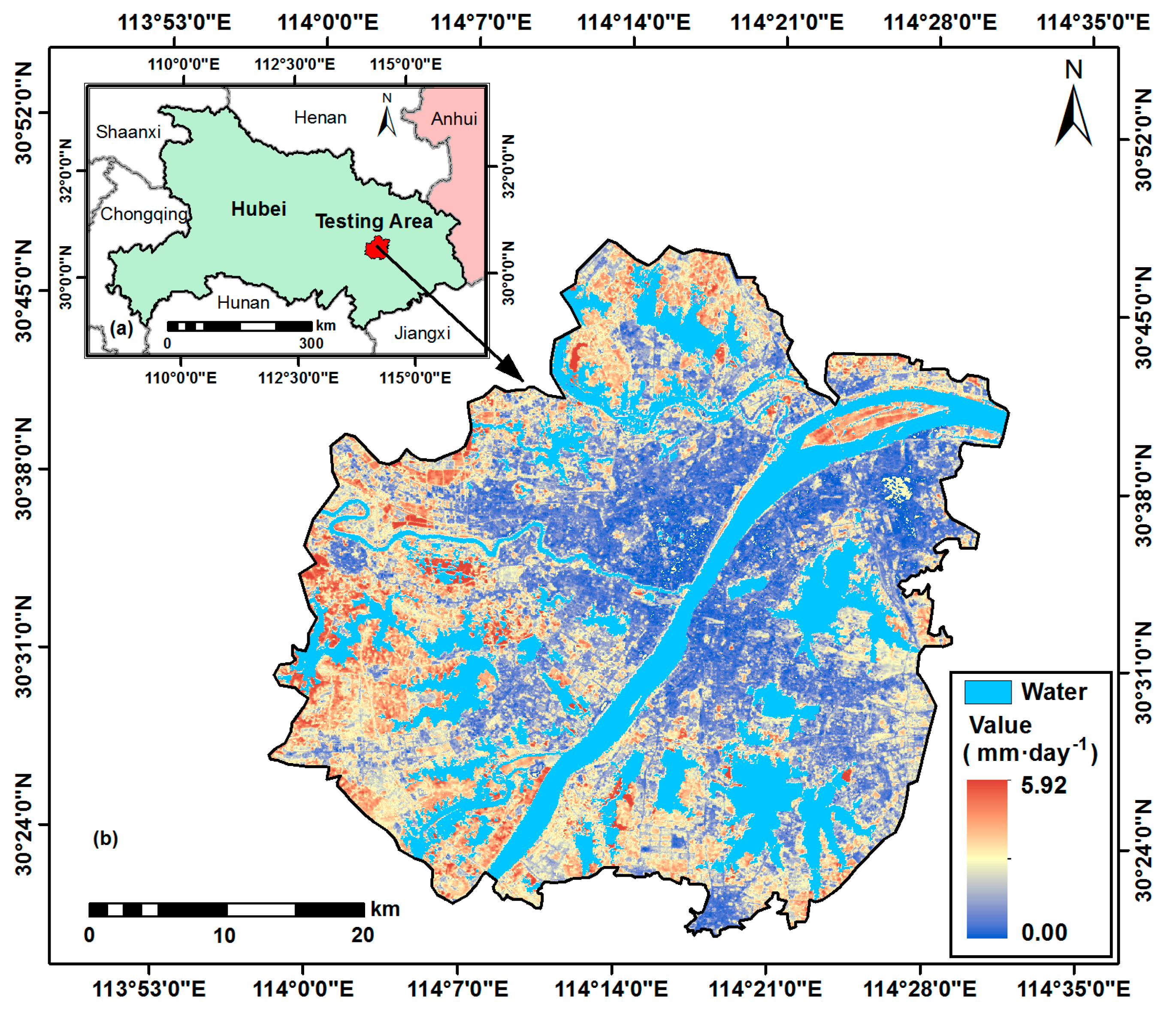
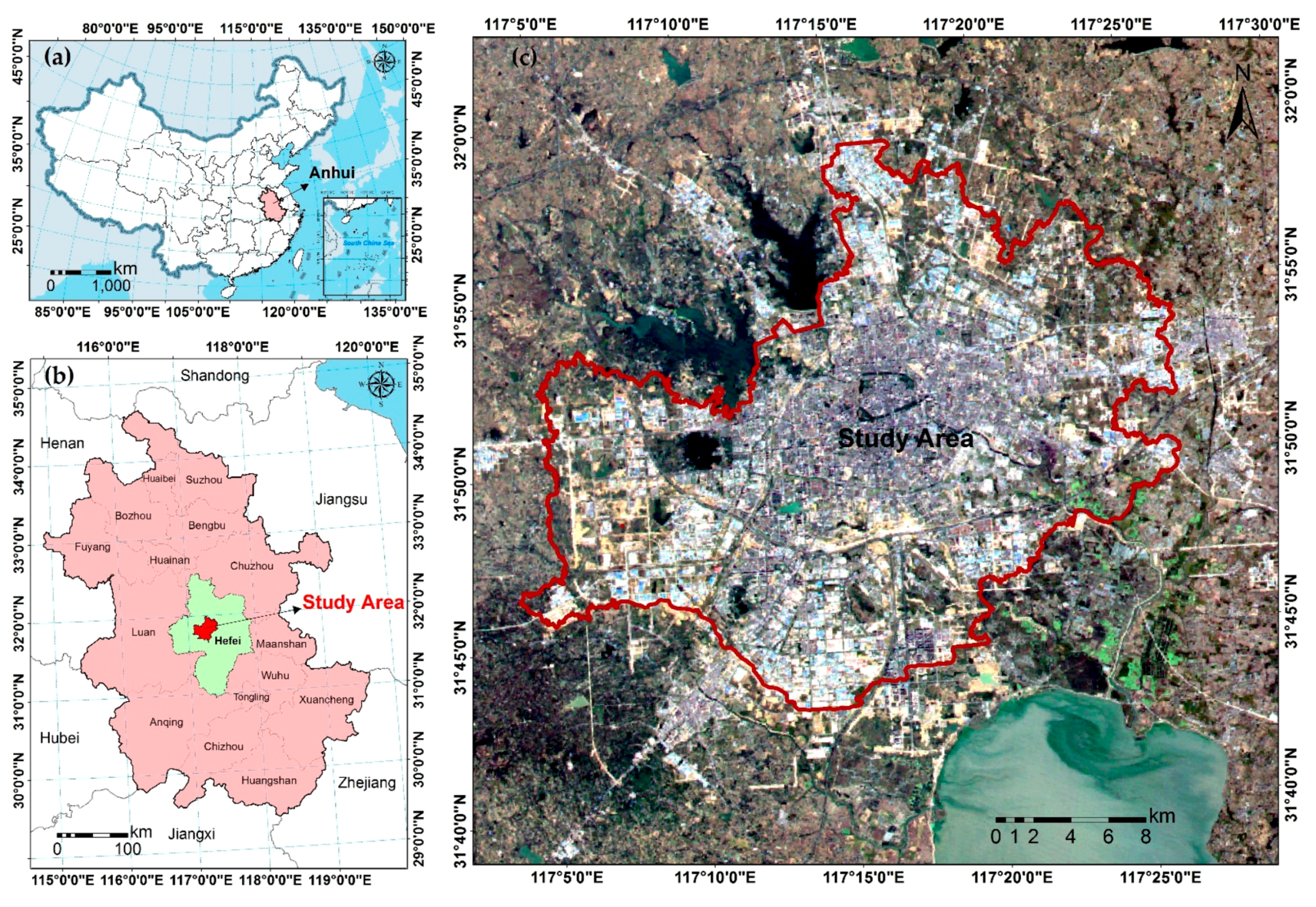
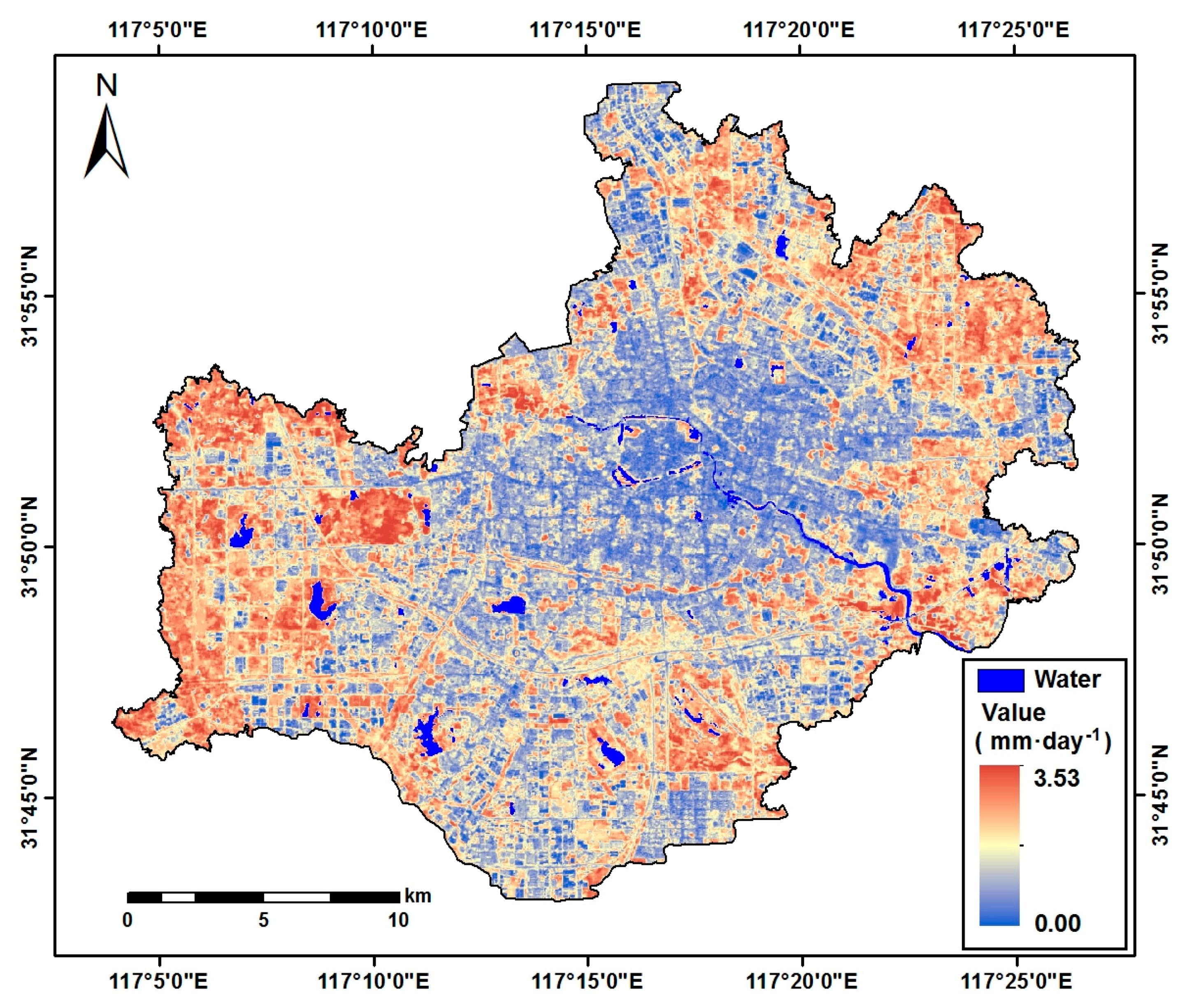
2.1. Study Area
2.2. Data and Preprocessing
3. Methodology
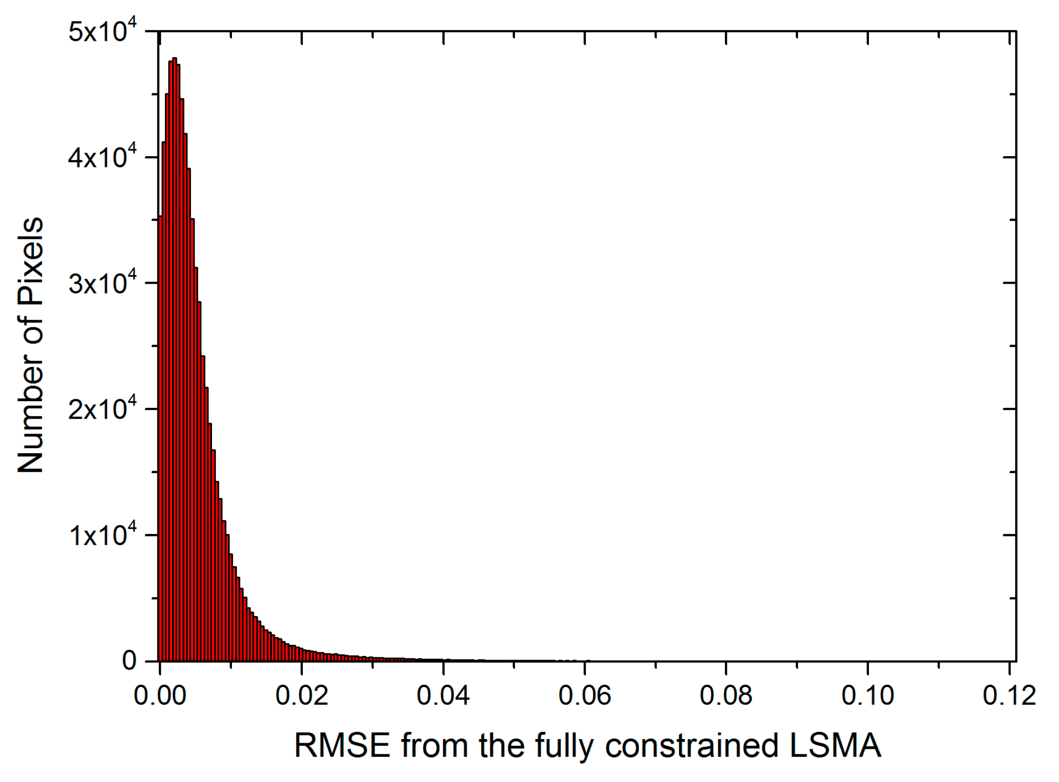
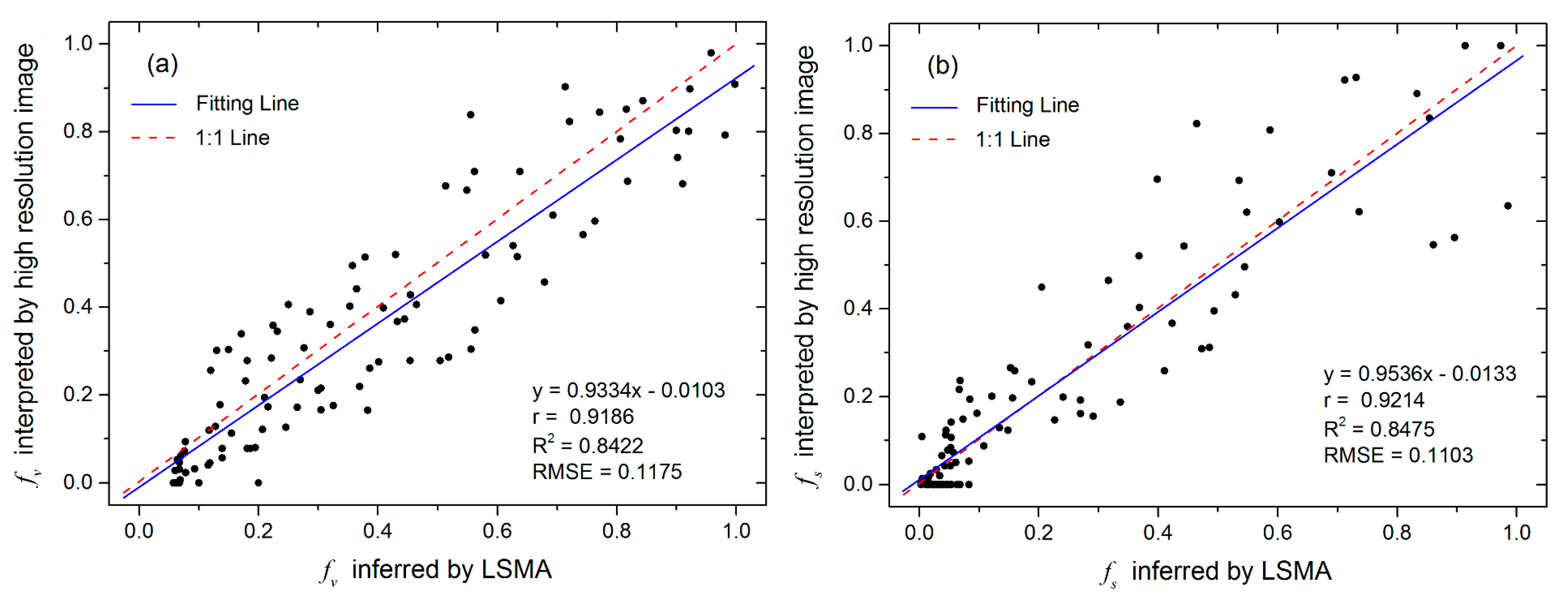
3.1. Linear Spectral Mixture Analysis
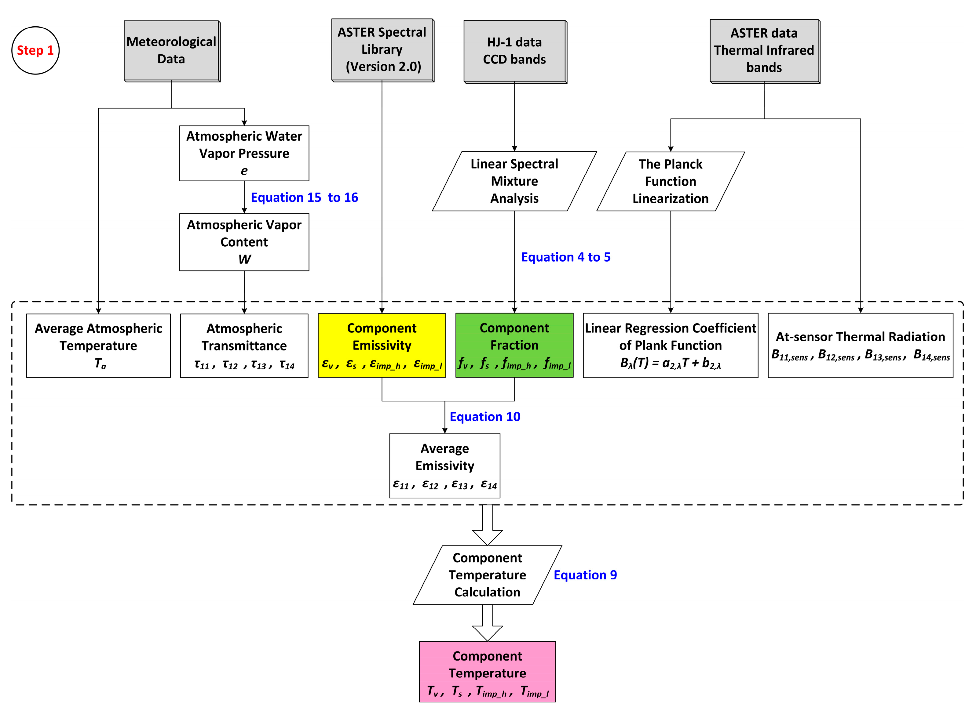
3.2. Retrieval of Land Surface Component Temperature
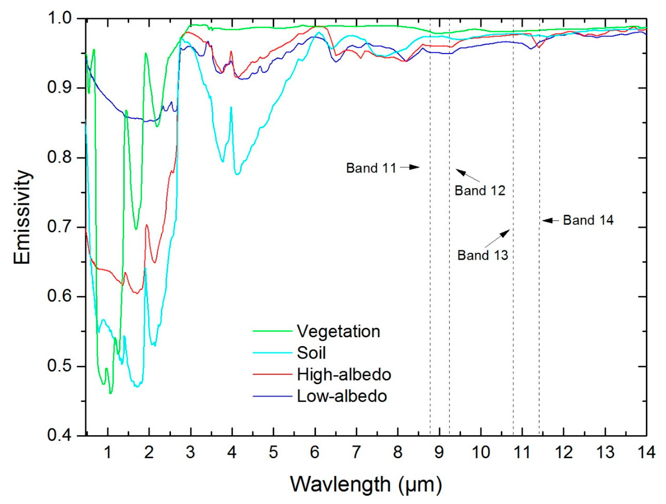
3.2.1. Average Land Surface Emissivity
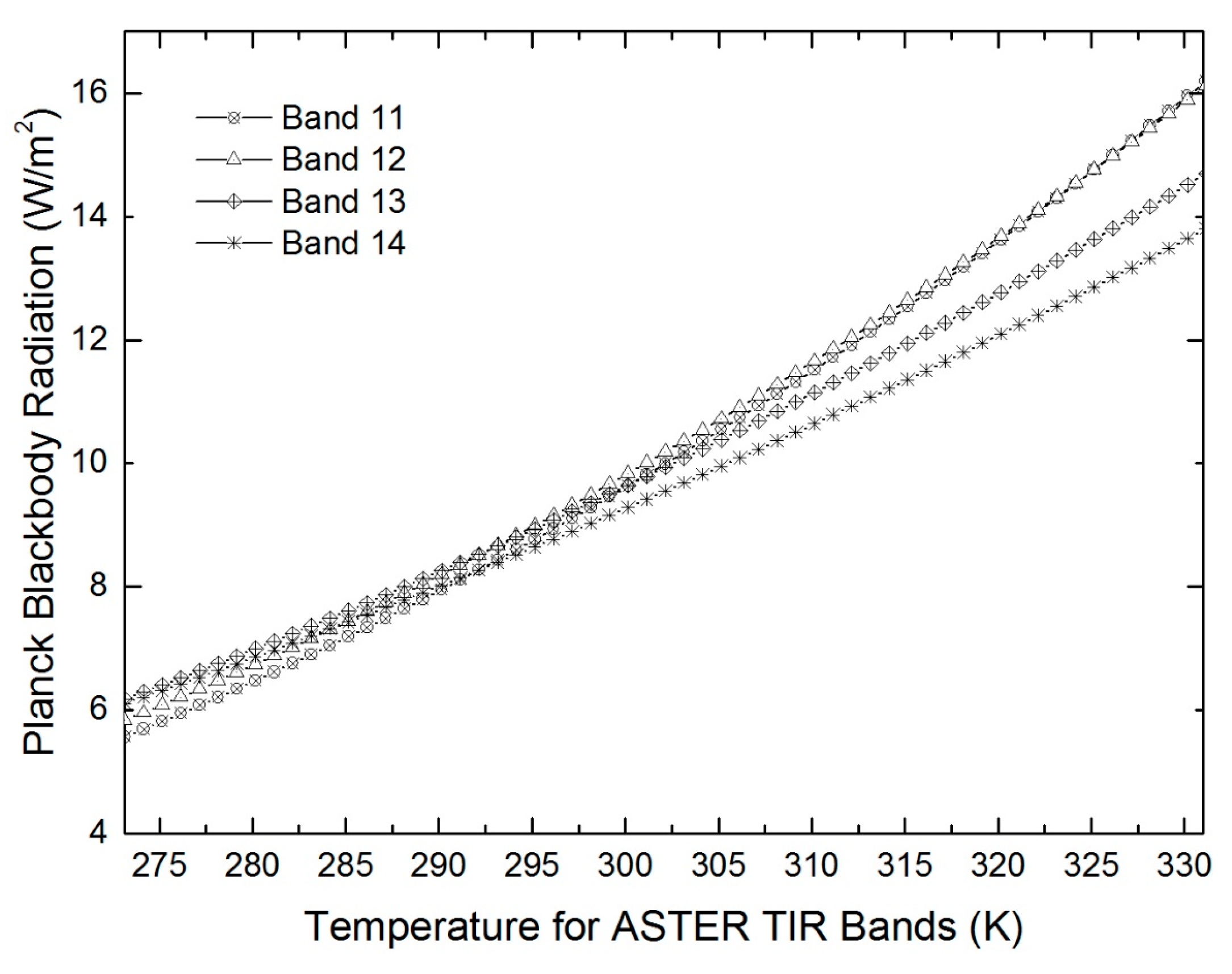
3.2.2. Atmospheric Transmittance for ASTER Thermal Infrared Bands
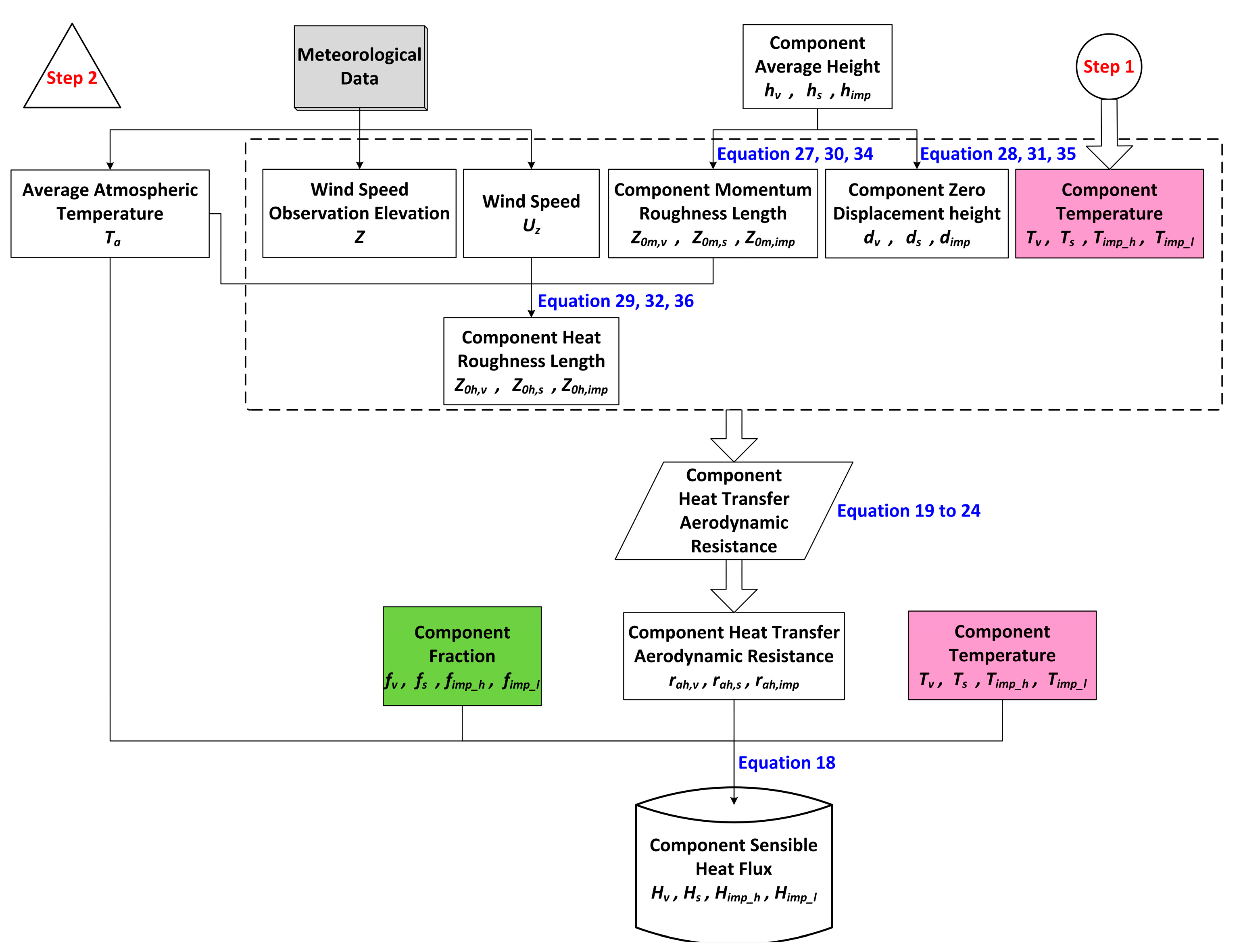
3.3. Retrieval of Land Surface Component Sensible Heat Flux
3.3.1. Aerodynamic Resistance to Heat Transfer
3.3.2. Momentum Roughness Length, Heat Roughness Length, and Zero Displacement Height
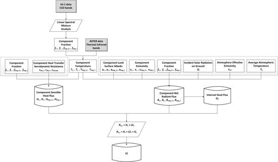
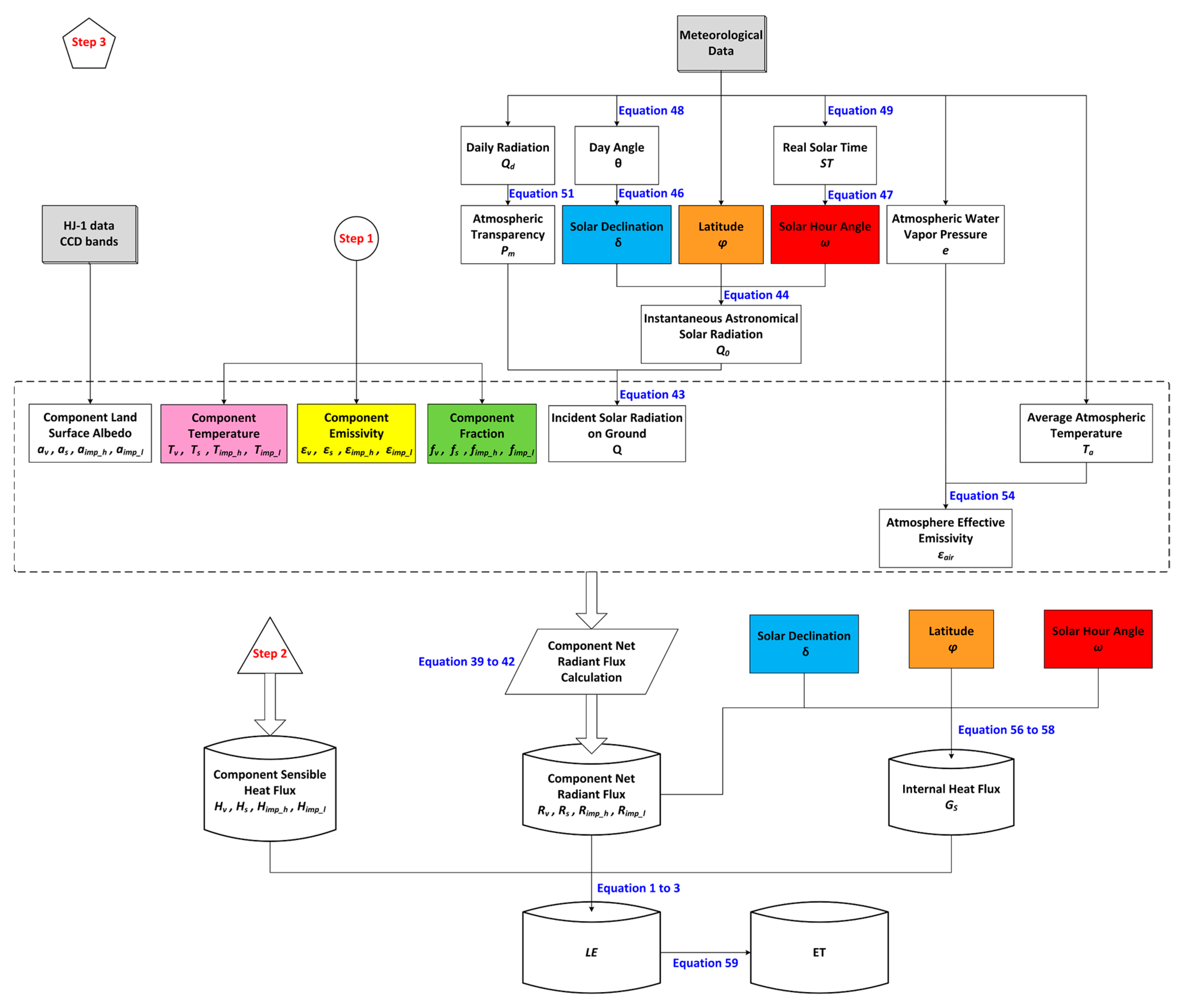
3.4. Retrieval of Land Surface Component Net Radiant Flux
3.4.1. Incident Solar Radiation on Ground
3.4.2. Atmosphere Effective Emissivity
3.4.3. Land Surface Albedo
3.5. Retrieval of Land Surface Component Internal Heat Flux
3.6. Retrieval of Daily Evapotranspiration
4. Results
5. Discussion
5.1. Using HJ-1A CCD VNIR Data Alternative to ASTER SWIR Data
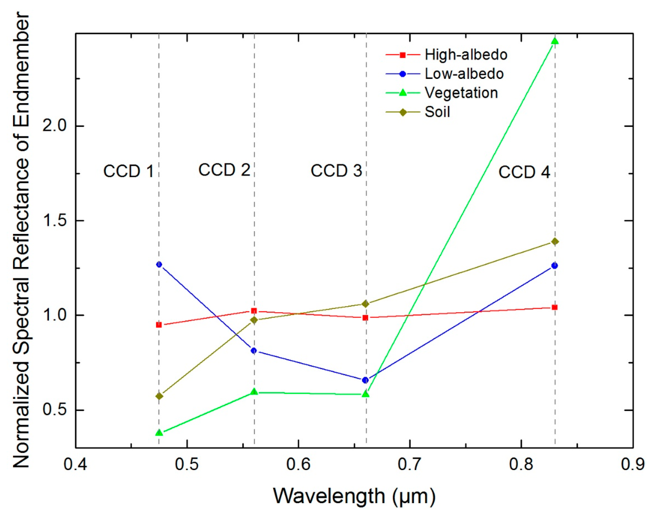
5.2. Optimized Endmembers of Urban Land Surface
5.3. Improved Parameterization of and
5.4. Algorithm Improvement of Component Net Radiant Flux
5.5. Sensitivity Analysis
5.6. Comparison with Other Models
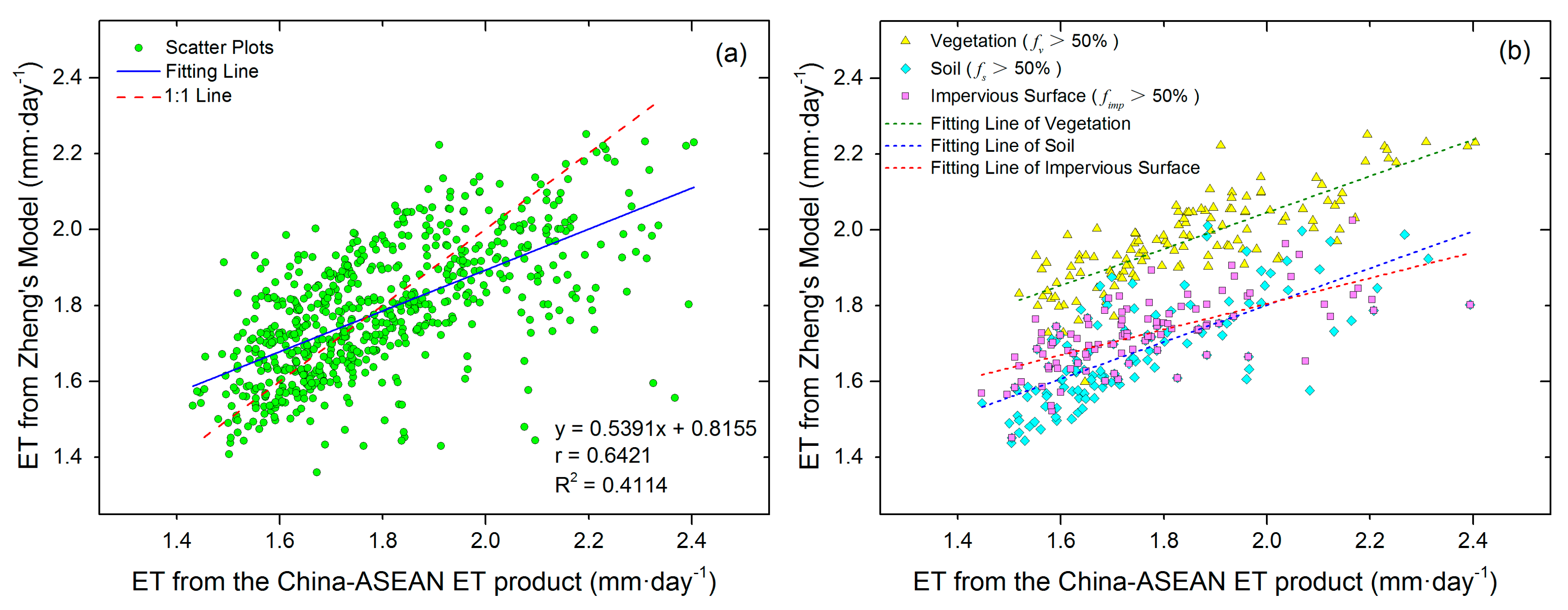
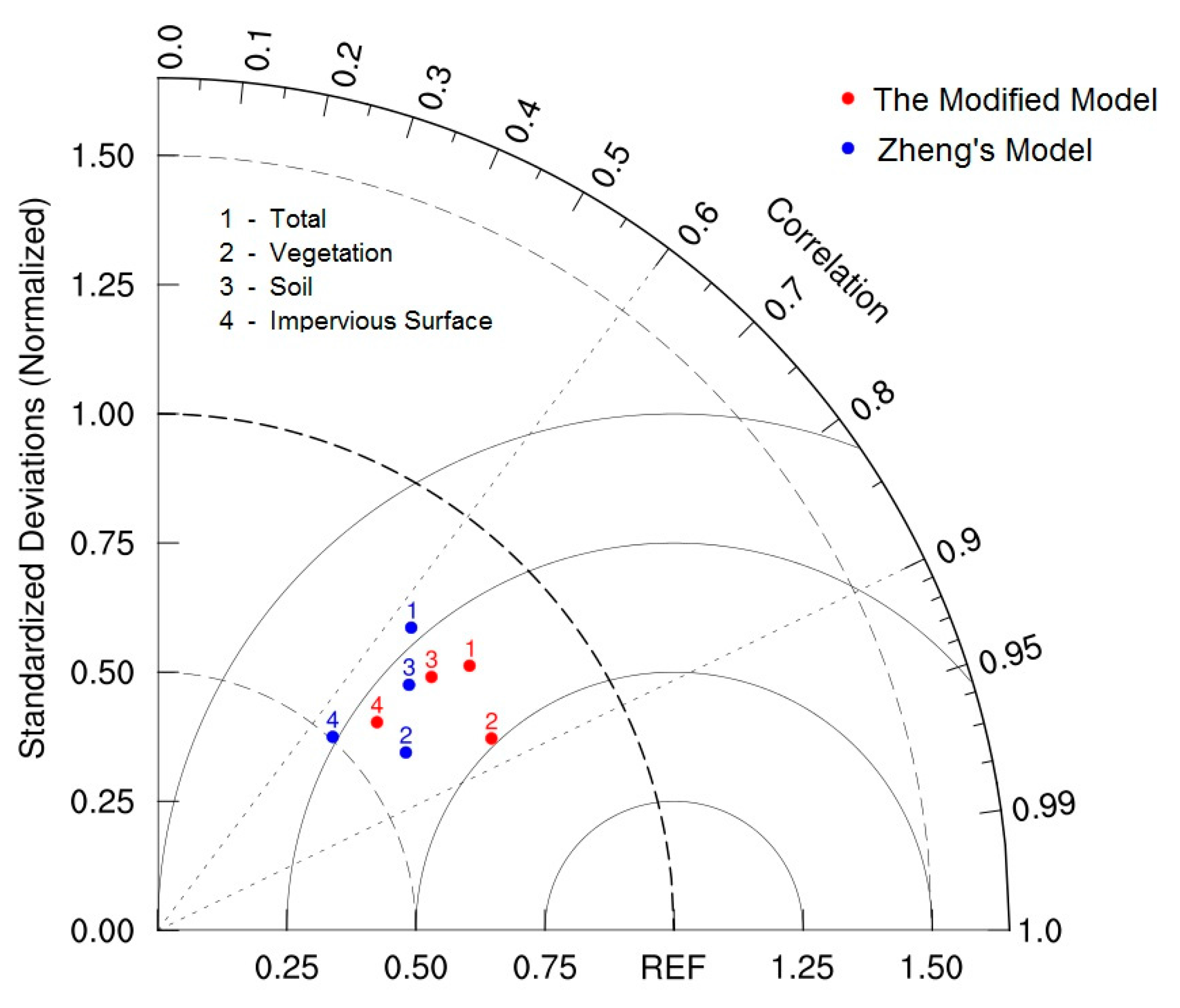
5.7. Comparison with Zheng’s Model
5.8. Applicability of Our Modified Model
6. Conclusions
- Instead of a single endmember, impervious surfaces are characterized by two different ones (high- and low-albedo) in linear spectral mixture analysis.
- Rather than constant empirical values, the roughness length for each land surface component (vegetation, soil, high- and low-albedo impervious surfaces) is calculated specifically to better approximate the real conditions of those land surfaces.
- Our model includes a new algorithm for estimating component net radiant flux by taking the fraction and characteristics of each land surface component into account.
Acknowledgments
Author Contributions
Conflicts of Interest
Appendix A

| Abbreviation of Variable | Meaning of Variable |
|---|---|
| Net radiant flux of vegetation | |
| Net radiant flux of soil | |
| Net radiant flux of impervious surface | |
| Sensible heat flux of vegetation | |
| Sensible heat flux of soil | |
| Sensible heat flux of impervious surface | |
| Latent heat flux of vegetation | |
| Latent heat flux of soil | |
| Soil heat flux | |
| Internal heat flux of impervious surface | |
| Component type, separately refer to vegetation, soil, high- and low-albedo impervious surface | |
| Pixel component fraction | |
| Pixel component temperature | |
| Reflectance for band in a pixel | |
| Reflectance of endmember for band in a pixel | |
| Thermal radiation of land surface at wavelength | |
| Land surface emissivity at wavelength | |
| Planck blackbody radiation when the land surface temperature is | |
| At-sensor thermal radiation at wavelength | |
| Atmospheric transmittance at wavelength | |
| Near-surface average atmospheric temperature | |
| Emissivity of component at wavelength | |
| Planck blackbody radiation of component at wavelength when the component temperature is | |
| Fraction of vegetation | |
| Fraction of soil | |
| Fraction of high-albedo impervious surface | |
| Fraction of low-albedo impervious surface | |
| The temperature ratio of vegetation | |
| The temperature ratio of soil | |
| The temperature ratio of man-made construction | |
| Vegetation coverage | |
| Atmospheric vapor content | |
| Average atmospheric water vapor | |
| Latitude of the center of the study area | |
| Average elevation of the study area | |
| Component sensible heat flux | |
| Air density | |
| Heat capacity of air at constant pressure | |
| Aerodynamic resistance to heat transfer of component | |
| Elevation at which wind speed is observed | |
| Zero displacement height | |
| Roughness lengths for momentum | |
| Roughness lengths for heat | |
| Von Karman's constant | |
| Wind speed | |
| Stability correction functions for momentum | |
| Stability correction functions for heat | |
| Monin–Obukhov length | |
| Gravitational acceleration | |
| Temperature scale with | |
| Friction velocity | |
| Component average height | |
| Roughness Reynolds number | |
| Kinematic molecular viscosity | |
| Solar shortwave radiation | |
| Solar longwave radiation | |
| Shortwave radiation reflected by the land surface | |
| Longwave radiation emitted by the land surface | |
| Albedo of the land surface | |
| Effective emissivity of the atmosphere | |
| Stefan Boltzmann constant | |
| Incident solar radiation on ground | |
| Component surface net radiant flux of vegetation | |
| Component surface net radiant flux of soil | |
| Component surface net radiant flux of high-albedo impervious surface | |
| Component surface net radiant flux of low-albedo impervious surface | |
| Atmospheric transmittance | |
| Air mass (solar radiation) | |
| Instantaneous astronomical solar radiation | |
| Solar constant | |
| Correction coefficient of sun-earth distance | |
| Solar declination | |
| Solar hour angle | |
| Day angle | |
| Real solar time | |
| Day number of the year | |
| Beijing time (UTC+8) | |
| Longitude of local standard time | |
| Local longitude | |
| Time lag | |
| Broad band albedo of HJ-1A CCD bands | |
| Internal heat flux of high-albedo impervious surface | |
| Internal heat flux of low-albedo impervious surface | |
| Sensible heat flux of vegetation | |
| Sensible heat flux of soil | |
| Sensible heat flux of high-albedo impervious surface | |
| Sensible heat flux of low-albedo impervious surface | |
| Latent heat of vaporization | |
| Evapotranspiration | |
| Instantaneous evapotranspiration | |
| Daily evapotranspiration | |
| Time interval from sunrise to the acquisition time of satellite imagery | |
| Evapotranspiration duration | |
| Taylor skill |
| Sensor | Acquisition Time (GMT) | Average Atmospheric Temperature (K) | Average Atmospheric Water Vapor Pressure (hpa) | Mean Wind Speed at 2 m Height (m/s) | Sunshine Duration (h) | Daily Incident Solar Radiation on Ground (MJ·m−2·d−1) |
|---|---|---|---|---|---|---|
| ASTER (TIR) | 2013-08-08 03:13:44 | 296.24 | 31.3 | 1.6 | 12.4 | 2698 |
| HJ-1B CCD1 (VNIR) | 2013-08-08 03:22:21 |
References
- Zhang, Q.; Qi, T.; Li, J.; Singh, V.P.; Wang, Z. Spatiotemporal variations of pan evaporation in China during 1960–2005: Changing patterns and causes. Int. J. Climatol. 2015, 35, 903–912. [Google Scholar] [CrossRef]
- Liu, X.; Shen, Y.; Li, H.; Guo, Y.; Pei, H.; Dong, W. Estimation of land surface evapotranspiration over complex terrain based on multi-spectral remote sensing data. Hydrol. Process. 2016, 1–16. [Google Scholar] [CrossRef]
- Sun, G.; Alstad, K.; Chen, J.; Chen, S.; Ford, C.R.; Lin, G.; Liu, C.; Lu, N.; McNulty, S.G.; Miao, H.; Noormets, A.; Vose, J.M.; Wilske, B.; Zeppel, M.; Zhang, Y.; Zhang, Z. A general predictive model for estimating monthly ecosystem evapotranspiration. Ecohydrology 2011, 4, 245–255. [Google Scholar] [CrossRef]
- Knipper, K.; Hogue, T.; Scott, R.; Franz, K. Evapotranspiration Estimates Derived Using Multi-Platform Remote Sensing in a Semiarid Region. Remote Sens. 2017, 9, 184. [Google Scholar] [CrossRef]
- Zheng, W. Inversion of Evapotranspiration on Urban Land Surface Based on Remote Sensing Data; Central South University: Changsha, China, 2012. (In Chinese) [Google Scholar]
- Verstraeten, W.W.; Veroustraete, F.; Feyen, J. Assessment of Evapotranspiration and Soil Moisture Content Across Different Scales of Observation. Sensors 2008, 8, 70–117. [Google Scholar] [CrossRef] [PubMed]
- Schmid, H.P.; Lloyd, C.R. Spatial representativeness and the location bias of flux footprints over inhomogeneous areas. Agric. For. Meteorol. 1999, 93, 195–209. [Google Scholar] [CrossRef]
- Alfieri, J.G.; Anderson, M.C.; Kustas, W.P.; Cammalleri, C. Effect of the revisit interval and temporal upscaling methods on the accuracy of remotely sensed evapotranspiration estimates. Hydrol. Earth Syst. Sci. 2017, 21, 83–98. [Google Scholar] [CrossRef]
- Cleugh, H.A.; Leuning, R.; Mu, Q.; Running, S.W. Regional evaporation estimates from flux tower and MODIS satellite data. Remote Sens. Environ. 2007, 106, 285–304. [Google Scholar] [CrossRef]
- Fisher, J.B.; Tu, K.P.; Baldocchi, D.D. Global estimates of the land-atmosphere water flux based on monthly AVHRR and ISLSCP-II data, validated at 16 FLUXNET sites. Remote Sens. Environ. 2008, 112, 901–919. [Google Scholar] [CrossRef]
- Jung, M.; Reichstein, M.; Bondeau, a. Towards global empirical upscaling of FLUXNET eddy covariance observations: validation of a model tree ensemble approach using a biosphere model. Biogeosciences Discuss. 2009, 6, 5271–5304. [Google Scholar] [CrossRef]
- Komatsu, H.; Cho, J.; Matsumoto, K.; Otsuki, K. Simple modeling of the global variation in annual forest evapotranspiration. J. Hydrol. 2012, 420–421, 380–390. [Google Scholar] [CrossRef]
- Yan, H.; Wang, S.Q.; Billesbach, D.; Oechel, W.; Zhang, J.H.; Meyers, T.; Martin, T.A.; Matamala, R.; Baldocchi, D.; Bohrer, G.; Dragoni, D.; Scott, R. Global estimation of evapotranspiration using a leaf area index-based surface energy and water balance model. Remote Sens. Environ. 2012, 124, 581–595. [Google Scholar] [CrossRef]
- Yao, Y.; Liang, S.; Li, X.; Chen, J.; Wang, K.; Jia, K.; Cheng, J.; Jiang, B.; Fisher, J.B.; Mu, Q.; Grünwald, T.; Bernhofer, C.; Roupsard, O. A satellite-based hybrid algorithm to determine the Priestley-Taylor parameter for global terrestrial latent heat flux estimation across multiple biomes. Remote Sens. Environ. 2015, 165, 216–233. [Google Scholar] [CrossRef]
- Bastiaanssen, W.G.M.; Meneti, M.; Feddes, R.A.; Holtslag, A.A.M. A remote sensing surface energy balance algorithm for land (SEBAL) 1.Formulation. J. Hydrol. 1998, 212–213, 198–212. [Google Scholar] [CrossRef]
- Allen, R.G.; Tasumi, M.; Trezza, R. Satellite-Based Energy Balance for Mapping Evapotranspiration with Internalized Calibration (METRIC)-Model. J. Irrig. Drain. Eng. 2007, 133, 380–394. [Google Scholar] [CrossRef]
- Allen, R.G.; Tasumi, M.; Morse, A.; Trezza, R.; Wright, J.L.; Bastiaanssen, W.; Kramber, W.; Lorite, I.; Robison, C.W. Satellite-Based Energy Balance for Mapping Evapotranspiration with Internalized Calibration (METRIC)-Applications. J. Irrig. Drain. Eng. 2007, 133, 395–406. [Google Scholar] [CrossRef]
- Su, Z. The Surface Energy Balance System (SEBS) for estimation of turbulent heat fluxes. Hydrol. Earth Syst. Sci. 2002, 6, 85–100. [Google Scholar] [CrossRef]
- Roerink, G.J.; Su, Z.; Menenti, M. S-SEBI: A simple remote sensing algorithm to estimate the surface energy balance. Phys. Chem. Earth, Part B Hydrol. Ocean. Atmos. 2000, 25, 147–157. [Google Scholar] [CrossRef]
- Sobrino, J.A.; Gómez, M.; Jiménez-Muñoz, J.C.; Olioso, A. Application of a simple algorithm to estimate daily evapotranspiration from NOAA-AVHRR images for the Iberian Peninsula. Remote Sens. Environ. 2007, 110, 139–148. [Google Scholar] [CrossRef]
- Shuttleworth, W.J.; Wallace, J.S. Evaporation From Spare Crops - An Energy Combination Theory. Q. J. R. Meteorol. Soc. 1985, 111, 839–855. [Google Scholar] [CrossRef]
- Shuttleworth, W.J.; Gurney, R.J. The theoretical relationship between foliage temperature and canopy resistance in sparse crops. Q. J. R. Meteorol. Soc. 1990, 116, 497–519. [Google Scholar] [CrossRef]
- Norman, J.M.; Kustas, W.P.; Humes, K.S. Source approach for estimating soil and vegetation energy fluxes in observations of directional radiometric surface temperature. Agric. For. Meteorol. 1995, 77, 263–293. [Google Scholar] [CrossRef]
- Kustas, W.P.; Norman, J.M. Evaluation of soil and vegetation heat flux predictions using a simple two-source model with radiometric temperatures for partial canopy cover. Agric. For. Meteorol. 1999, 94, 13–29. [Google Scholar] [CrossRef]
- Norman, J.M.; Kustas, W.P.; Prueger, J.H.; Diak, G.R. Surface flux estimation using radiometric temperature: A dual temperature-difference method to minimize measurement errors. Water Resour. Res. 2000, 36, 2263–2274. [Google Scholar] [CrossRef]
- Anderson, M.C.; Norman, J.M.; Diak, G.R.; Kustas, W.P.; Mecikalski, J.R. A two-source time-integrated model for estimating surface fluxes using thermal infrared remote sensing. Remote Sens. Environ. 1997, 60, 195–216. [Google Scholar] [CrossRef]
- Anderson, M.C.; Norman, J.M.; Mecikalski, J.R.; Otkin, J.A.; Kustas, W.P. A climatological study of evapotranspiration and moisture stress across the continental United States based on thermal remote sensing: 1. Model formulation. J. Geophys. Res. Atmos. 2007, 112, 1–17. [Google Scholar] [CrossRef]
- Anderson, M.C.; Norman, J.M.; Mecikalski, J.R.; Otkin, J.A.; Kustas, W.P. A climatological study of evapotranspiration and moisture stress across the continental United States based on thermal remote sensing: 2. Surface moisture climatology. J. Geophys. Res. Atmos. 2007, 112, 1–13. [Google Scholar] [CrossRef]
- Long, D.; Singh, V.P. A Two-source Trapezoid Model for Evapotranspiration (TTME) from satellite imagery. Remote Sens. Environ. 2012, 121, 370–388. [Google Scholar] [CrossRef]
- Wu, C.; Murray, A.T. Estimating impervious surface distribution by spectral mixture analysis. Remote Sens. Environ. 2003, 84, 493–505. [Google Scholar] [CrossRef]
- Qin, R.X.; Xiao, C.; Zhu, Y.; Li, J.; Yang, J.; Gu, S.; Xia, J.; Su, B.; Liu, Q.; Woodward, A. The interactive effects between high temperature and air pollution on mortality: A time-series analysis in Hefei, China. Sci. Total Environ. 2016, 575, 1530–1537. [Google Scholar] [CrossRef] [PubMed]
- NASA Jet Propulsion Laboratory. Available online: https://asterweb.jpl.nasa.gov/swir-alert.asp (accessed on 15 February 2017).
- MODIS Global Evapotranspiration Project (MOD16). Available online: http://www.ntsg.umt.edu/project/mod16 (accessed on 27 March 2017).
- Mu, Q.; Heinsch, F.A.; Zhao, M.; Running, S.W. Development of a global evapotranspiration algorithm based on MODIS and global meteorology data. Remote Sens. Environ. 2007, 111, 519–536. [Google Scholar] [CrossRef]
- Global Change Research Data Publishing & Repository. Available online: http://www.geodoi.ac.cn/WebEn/doi.aspx?Id=206 (accessed on 28 March 2017).
- Hinkle, D.E.; Wiersma, W.; Jurs, S.G. Applied Statistics for the Behavioral Sciences, 5th ed.; Houghton Mifflin: Boston, MA, USA, 2003. [Google Scholar]
- Mukaka, M.M. A guide to appropriate use of Correlation coefficient in medical research. Malawi Med. J. 2012, 24, 69–71. [Google Scholar] [PubMed]
- Kustas, W.P.; Moran, M.S.; Humes, K.S.; Stannard, D.I.; Pinter, P.J.; Hipps, L.E.; Swiatek, E.; Goodrich, D.C. Surface energy balance estimates at local and regional scales using optical remote sensing from an aircraft platform and atmospheric data collected over semiarid rangelands. Water Resour. Res. 1994, 30, 1241–1259. [Google Scholar] [CrossRef]
- Li, L.; Canters, F.; Solana, C.; Ma, W.; Chen, L.; Kervyn, M. Discriminating lava flows of different age within Nyamuragira’s volcanic field using spectral mixture analysis. Int. J. Appl. Earth Obs. Geoinf. 2015, 40, 1–10. [Google Scholar] [CrossRef]
- Heinz, D.C.; Chang, C.I. Fully constrained least squares linear spectral mixture analysis method for material quantification in hyperspectral imagery. IEEE Trans. Geosci. Remote Sens. 2001, 39, 529–545. [Google Scholar] [CrossRef]
- Small, C. Estimation of urban vegetation abundance by spectral mixture analysis. Int. J. Remote Sens. 2001, 22, 1305–1334. [Google Scholar] [CrossRef]
- Wu, C. Normalized spectral mixture analysis for monitoring urban composition using ETM+ imagery. Remote Sens. Environ. 2004, 93, 480–492. [Google Scholar] [CrossRef]
- Demarchi, L.; Canters, F.; Chan, J.C.W.; Van De Voorde, T. Multiple endmember unmixing of CHRIS/proba imagery for mapping impervious surfaces in urban and suburban environments. IEEE Trans. Geosci. Remote Sens. 2012, 50, 3409–3424. [Google Scholar] [CrossRef]
- Van de Voorde, T.; De Roeck, T.; Canters, F. A comparison of two spectral mixture modelling approaches for impervious surface mapping in urban areas. Int. J. Remote Sens. 2009, 30, 4785–4806. [Google Scholar] [CrossRef]
- Plaza, A.; Martínez, P.; Pérez, R.; Plaza, J. A quantitative and comparative analysis of endmember extraction algorithms from hyperspectral data. IEEE Trans. Geosci. Remote Sens. 2004, 42, 650–663. [Google Scholar] [CrossRef]
- Martínez, P.J.; Pérez, R.M.; Plaza, A.; Aguilar, P.L.; Cantero, M.C.; Plaza, J. Endmember extraction algorithms from hyperspectral images. Ann. Geophys. 2006, 49, 93–101. [Google Scholar]
- Chang, C.I.; Plaza, A. A fast iterative algorithm for implementation of pixel purity index. IEEE Geosci. Remote Sens. Lett. 2006, 3, 63–67. [Google Scholar] [CrossRef]
- VAN DE GRIEND, A.A.; OWE, M. On the relationship between thermal emissivity and the normalized difference vegetation index for natural surfaces. Int. J. Remote Sens. 1993, 14, 1119–1131. [Google Scholar] [CrossRef]
- Qin, Z.; Karnieli, A.; Berliner, P. A mono-window algorithm for retrieving land surface temperature from Landsat TM data and its application to the Israel-Egypt border region. Int. J. Remote Sens. 2001, 22, 3719–3746. [Google Scholar] [CrossRef]
- Song, X.; Zhao, Y. Study on component temperatures inversion using satellite remotely sensed data. Int. J. Remote Sens. 2007, 28, 2567–2579. [Google Scholar] [CrossRef]
- COLL, C.; CASELLES, V.; SOBRINO, J.A.; VALOR, E. On the atmospheric dependence of the split-window equation for land surface temperature. Int. J. Remote Sens. 1994, 15, 105–122. [Google Scholar] [CrossRef]
- Mao, K.; Qin, Z.; Shi, J.; Gong, P. A practical split-window algorithm for retrieving land-surface temperature from MODIS data. Int. J. Remote Sens. 2005, 26, 3181–3204. [Google Scholar] [CrossRef]
- Qin, Z.; Li, W.; Xu, B.; Chen, Z.; Liu, J. The estimation of land surface emissivity for landsat TM6. Remote Sens. L. Resour. 2004, 28–42. (In Chinese) [Google Scholar]
- Howell, J.R.; Menguc, M.P.; Siegel, R. Thermal Radiation Heat Transfer, 5th ed.; Cambridge University Press: Cambridge, UK, 2010. [Google Scholar]
- ASTER Spectral Library. Available online: https://speclib.jpl.nasa.gov/ (accessed on 14 March 2017).
- Mao, K.; Shi, J.; Qin, Z.; Peng, G.; Xu, B.; Jiang, L. A Four-Channel Algorithm for Retrieving Land Surface Temperature and Emissivity from ASTER Data. J. Remote Sens. 2006, 10, 593–599. (In Chinese) [Google Scholar]
- Yang, J.; Qiu, J. A Method for Estimating Precipitable Water and Effective Water Vapor Content from Ground Humidity Parameters. Chin. J. Atmos. Sci. 2002, 26, 9–22. (In Chinese) [Google Scholar]
- China Meteorological Data Network. Available online: http://data.cma.cn/ (accessed on 17 March 2017).
- Monteith, J.L.; Unsworth, M.H. Principles of Environmental Physics. In Principles of Environmental Physics; Elsevier: Amsterdam, 2013; pp. 151–152. [Google Scholar]
- Businger, J.A. A note on the Businger-Dyer profiles. Boundary-Layer Meteorol. 1988, 42, 145–151. [Google Scholar] [CrossRef]
- Sugita, M.; Brutsaert, W. Regional Surface Fluxes From Remotely Sensed Skin Temperature and Lower Boundary-Layer Measurements. Water Resour. Res. 1990, 26, 2937–2944. [Google Scholar] [CrossRef]
- Zhang, Y.; Liu, C.; Lei, Y.; Tang, Y.; Yu, Q.; Shen, Y.; Sun, H. An integrated algorithm for estimating regional latent heat flux and daily evapotranspiration. Int. J. Remote Sens. 2006, 27, 129–152. [Google Scholar] [CrossRef]
- Kanda, M.; Kanega, M.; Kawai, T.; Moriwaki, R.; Sugawara, H. Roughness lengths for momentum and heat derived from outdoor urban scale models. J. Appl. Meteorol. Climatol. 2007, 46, 1067–1079. [Google Scholar] [CrossRef]
- Kustas, W.P.; Choudhury, B.J.; Moran, M.S.; Reginato, R.J.; Jackson, R.D.; Gay, L.W.; Weaver, H.L. Determination of sensible heat flux over sparse canopy using thermal infrared data. Agric. For. Meteorol. 1989, 44, 197–216. [Google Scholar] [CrossRef]
- Wang, J.D.; Li, X.W.; Sun, X.M.; Liu, Q. Component temperatures inversion for remote sensing pixel based on directional thermal radiation model. Sci. China Ser. E-Technol. Sci. 2000, 43, 41–47. [Google Scholar] [CrossRef]
- Grimmond, C.S.B.; Oke, T.R. Aerodynamic Properties of Urban Areas Derived from Analysis of Surface Form. J. Appl. Meteorol. 1999, 38, 1262–1292. [Google Scholar] [CrossRef]
- Gao, Z.; Bian, L.; Lu, C.; Lu, L.; Wang, J.; Wang, Y. Estimation of Aerodynamic Parameters in Urban Areas. J. Appl. Meteorl. Sci. 2002, 13, 26–33. (in Chinese). [Google Scholar]
- Nadeau, D.F.; Brutsaert, W.; Parlange, M.B.; Bou-Zeid, E.; Barrenetxea, G.; Couach, O.; Boldi, M.O.; Selker, J.S.; Vetterli, M. Estimation of urban sensible heat flux using a dense wireless network of observations. Environ. Fluid Mech. 2009, 9, 635–653. [Google Scholar] [CrossRef]
- Voogt, J.A.; Grimmond, C.S.B. Modeling Surface Sensible Heat Flux Using Surface Radiative Temperatures in a Simple Urban Area. J. Appl. Meteorol. 1999, 39, 1679–1699. [Google Scholar] [CrossRef]
- Liu, S.; Lu, L.; Mao, D.; Jia, L. Evaluating parameterizations of aerodynamic resistance to heat transfer using field measurements. Hydrol. Earth Syst. Sci. 2007, 11, 769–783. [Google Scholar] [CrossRef]
- Stewart, J.B.; Kustas, W.P.; Humes, K.S.; Nichols, W.D.; Moran, M.S.; Debruin, H.A.R. Sensible Heat-Flux Radiometric Surface-Temperature Relationship for 8 Semiarid Areas. J. Appl. Meteorol. 1994, 33, 1110–1117. [Google Scholar] [CrossRef]
- Moran, M.S.; Jackson, R.D.; Raymond, L.H.; Gay, L.W.; Slater, P.N. Mapping Surface Energy Balance Components by Combining Landsat Thematic Mapper and Ground-Based Meteorological Data. Remote Sens. Environ. 1989, 87, 77–87. [Google Scholar] [CrossRef]
- Ambast, S.K.; Keshari, A.K.; Gosain, A.K. An operational model for estimating Regional Evapotranspiration through Surface Energy Partitioning (RESEP). Int. J. Remote Sens. 2002, 23, 4917–4930. [Google Scholar] [CrossRef]
- Yang, Y.; Su, H.; Zhang, R.; Tian, J.; Li, L. An enhanced two-source evapotranspiration model for land (ETEML): Algorithm and evaluation. Remote Sens. Environ. 2015, 168, 54–65. [Google Scholar] [CrossRef]
- Wang, B.; Pan, G. The transparency of atmosphere over China and its computation. Acta Energ. Sol. Sin. 1981, 2, 13–22. (In Chinese) [Google Scholar]
- Angot, A. Recherches théoriques sur la distrirution de la chaleur à la surface du globe. J. Phys. Theor. Appl. 1886, 5, 5–16. [Google Scholar] [CrossRef]
- Milankovitch, M. Mathematische Klimalehre und astronomische Theorie der Klimaschwankungen; Schweizerbart Science Publishers: Stuttgart, Germany, 1930. [Google Scholar]
- Gueymard, C.A.; Myers, D.; Emery, K. Proposed reference irradiance spectra for solar energy systems testing. Sol. Energy 2002, 73, 443–467. [Google Scholar] [CrossRef]
- Gonzalez, C.; Ross, R. Performance measurement reference conditions for terrestrial photovoltaics. In Proceedings of the International Solar Energy Society Conference, Pasadena, CA, USA, 2 June 1980. [Google Scholar]
- Sheng, P.; Mao, J.; Li, J.; Zhang, A.; Sang, J.; Pan, N. Atmospheric Physics; Beijing University Press: Beijing, China, 2003. (In Chinese) [Google Scholar]
- Wong, L.T.; Chow, W.K. Solar radiation model. Appl. Energy 2001, 69, 191–224. [Google Scholar] [CrossRef]
- Malek, E. Evaluation of effective atmospheric emissivity and parameterization of cloud at local scale. Atmos. Res. 1997, 45, 41–54. [Google Scholar] [CrossRef]
- Brutsaert, W. On a derivable formula for longwave radiation from clear skies. Water Resour. Res. 1975, 11, 742–744. [Google Scholar] [CrossRef]
- Gao, B.; Gong, H.; Wang, T. A method for retrieving daily land surface albedo from space at 30-m resolution. Remote Sens. 2015, 7, 10951–10972. [Google Scholar] [CrossRef]
- Friedl, M.A. Relationships among remotely sensed data, surface energy balance, and area-averaged fluxes over partially vegetated land surfaces. J. Appl. Meteorol. 1996, 35, 2091–2103. [Google Scholar] [CrossRef]
- Mahour, M.; Stein, A.; Sharifi, A.; Tolpekin, V. Integrating super resolution mapping and SEBS modeling for evapotranspiration mapping at the field scale. Precis. Agric. 2015, 16, 571–586. [Google Scholar] [CrossRef]
- Xie, X. Estimation of daily evapotranspiration (ET) from one time-of-day remotely sensed canopy temperature. J. Remote Sens. 1991, 6, 253–260. (In Chinese) [Google Scholar]
- Luo, K.; Tao, F. Monitoring of forest virtual water in Hunan Province, China, based on HJ-CCD remote-sensing images and pattern analysis. Int. J. Remote Sens. 2016, 37, 2376–2393. [Google Scholar] [CrossRef]
- Deng, Y.; Wu, C. Development of a Class-Based Multiple Endmember Spectral Mixture Analysis (C-MESMA) Approach for Analyzing Urban Environments. Remote Sens. 2016, 8, 349. [Google Scholar] [CrossRef]
- De Ridder, K. Testing Brutsaert’s temperature roughness parameterization for representing urban surfaces in atmospheric models. Geophys. Res. Lett. 2006, 33, 12–15. [Google Scholar] [CrossRef]
- Liou, Y.A.; Kar, S.K. Evapotranspiration estimation with remote sensing and various surface energy balance algorithms-a review. Energies 2014, 7, 2821–2849. [Google Scholar] [CrossRef]
- Su, H.; McCabe, M.F.; Wood, E.F.; Su, Z.; Prueger, J.H. Modeling Evapotranspiration during SMACEX: Comparing Two Approaches for Local-and Regional-Scale Prediction. J. Hydrometeorol. 2009, 6, 1–13. [Google Scholar] [CrossRef]
- Bastiaanssen, W.; Noordman, E.J.; Pelgrum, H.; Davids, G.; Thoreson, B.; Allen, R.G. SEBAL Model with Remotely Sensed Data to Improve Water-Resources Management under Actual Field Conditions. J. Irrig. Drain. Eng. 2005, 131, 2. [Google Scholar] [CrossRef]
- Allen, R.G.; Tasumi, M.; Morse, A.; Trezza, R. A landsat-based energy balance and evapotranspiration model in Western US water rights regulation and planning. Irrig. Drain. Syst. 2005, 19, 251–268. [Google Scholar] [CrossRef]
- Gowda, P.H.; Chävez, J.; Howell, T.A.; Marek, T.H.; New, L.L. Surface energy balance based evapotranspiration mapping in the Texas high plains. Sensors 2008, 8, 5186–5201. [Google Scholar] [CrossRef] [PubMed]
- Taylor, K.E. Summarizing multiple aspects of model performance in a single diagram. J. Geophys. Res. Atmos. 2001, 106, 7183–7192. [Google Scholar] [CrossRef]
- Zhang, Y.; Chen, L.; Wang, Y.; Chen, L.; Yao, F.; Wu, P.; Wang, B.; Li, Y.; Zhou, T.; Zhang, T. Research on the Contribution of Urban Land Surface Moisture to the Alleviation Effect of Urban Land Surface Heat Based on Landsat 8 Data. Remote Sens. 2015, 7, 10737–10762. [Google Scholar] [CrossRef]
- Chen, J.; Chen, B.; Black, T.A.; Innes, J.L.; Wang, G.; Kiely, G.; Hirano, T.; Wohlfahrt, G. Comparison of terrestrial evapotranspiration estimates using the mass transfer and Penman-Monteith equations in land surface models. J. Geophys. Res. Biogeosciences 2013, 118, 1715–1731. [Google Scholar] [CrossRef]


| Sensor | Band | Wavelength (μm) | Resolution (m) | Revisit Cycle (day) | Acquisition Time (GMT) | Acquisition Date |
|---|---|---|---|---|---|---|
| ASTER (TIR) | 10 | 8.125–8.475 | 90 | 16 | 03:00:43 | 13 October 2017 |
| 11 | 8.475–8.825 | |||||
| 12 | 8.925–9.275 | |||||
| 13 | 10.25–10.95 | |||||
| 14 | 10.95–11.65 | |||||
| HJ-1A CCD2 (VNIR) | 1 | 0.43–0.52 | 30 | 2 | 01:57:19 | 13 October 2017 |
| 2 | 0.52–0.60 | |||||
| 3 | 0.63–0.69 | |||||
| 4 | 0.76–0.90 |
| Band | R2 | ||
|---|---|---|---|
| 11 | 0.19450 | −48.602 | 0.9953 |
| 12 | 0.18754 | −46.329 | 0.9960 |
| 13 | 0.14532 | −33.685 | 0.9966 |
| 14 | 0.13266 | −30.273 | 0.9972 |
| Band () | Vegetation Emissivity () | Soil Emissivity () | High-Albedo Impervious Surface Emissivity () | Low-Albedo Impervious Surface Emissivity () |
|---|---|---|---|---|
| 11 | 0.9838 | 0.9764 | 0.9627 | 0.9574 |
| 12 | 0.9788 | 0.9755 | 0.9606 | 0.9493 |
| 13 | 0.9812 | 0.9781 | 0.9762 | 0.9665 |
| 14 | 0.9829 | 0.9764 | 0.9670 | 0.9595 |
| Band | R2 | ||
|---|---|---|---|
| 11 | −0.068 | 0.9468 | 0.9983 |
| 12 | −0.066 | 0.9475 | 0.9975 |
| 13 | −0.074 | 0.9840 | 0.9845 |
| 14 | −0.100 | 1.0110 | 0.9899 |
| Acquisition Date | Average Atmospheric Temperature (K) | Average Atmospheric Water Vapor Pressure (hPa) | Mean Wind Speed at 2 m Height (m/s) | Sunshine Duration (h) |
|---|---|---|---|---|
| 2013-10-13 | 295.35 | 15.8 | 2.1 | 10.3 |
| Land Surface Component | Albedo |
|---|---|
| Vegetation | 0.18 |
| Soil | 0.28 |
| High-albedo impervious surfaces | 0.15 |
| Low-albedo impervious surfaces | 0.12 |
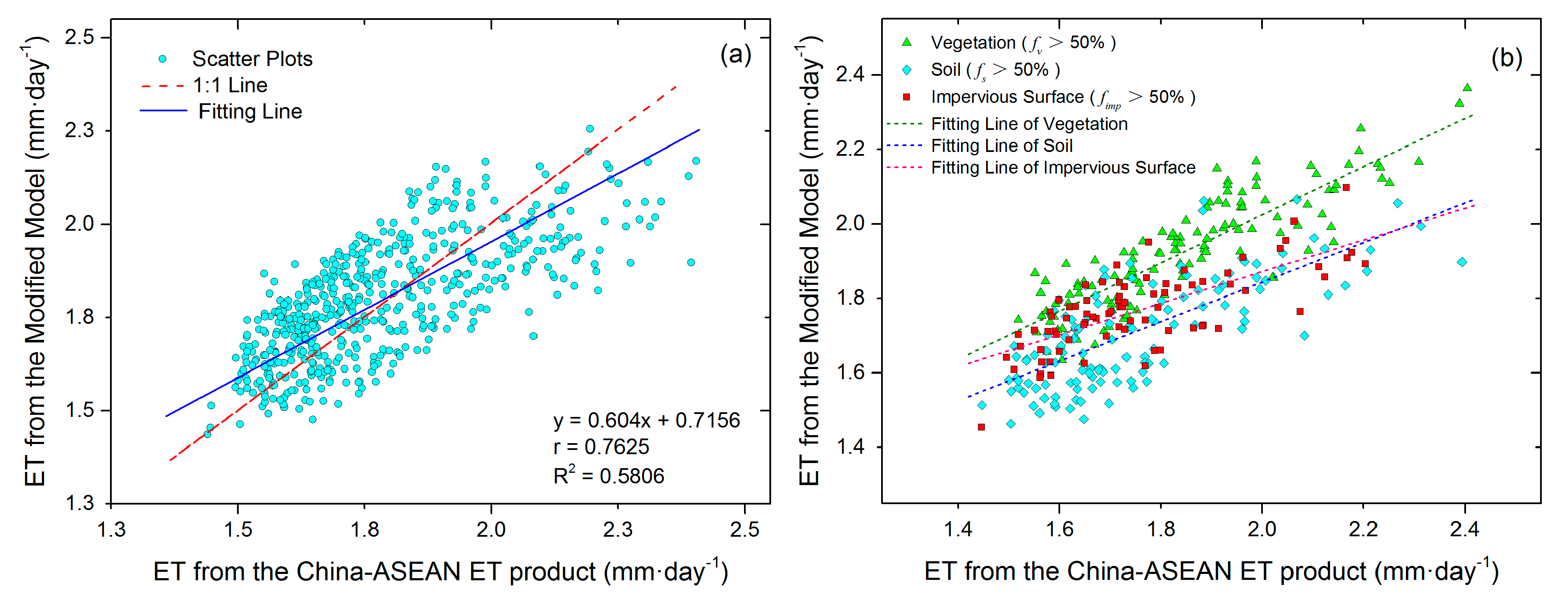
| Accuracy Measures | Correlation Coefficient (r) | Regression Equation | R2 | Mean Relative Error (MRE) | Root Mean Square Error (RMSE) | |
|---|---|---|---|---|---|---|
| Land Cover Type | ||||||
| Vegetation | 0.8669 | 0.7495 | 6.08% | 0.1281 | ||
| Soil | 0.7339 | 0.5349 | 6.12% | 0.1370 | ||
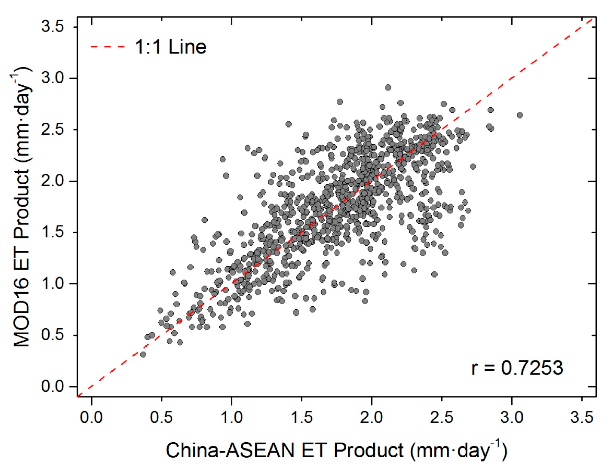
| Impervious surfaces | 0.7253 | 0.5200 | 5.90% | 0.1274 | ||
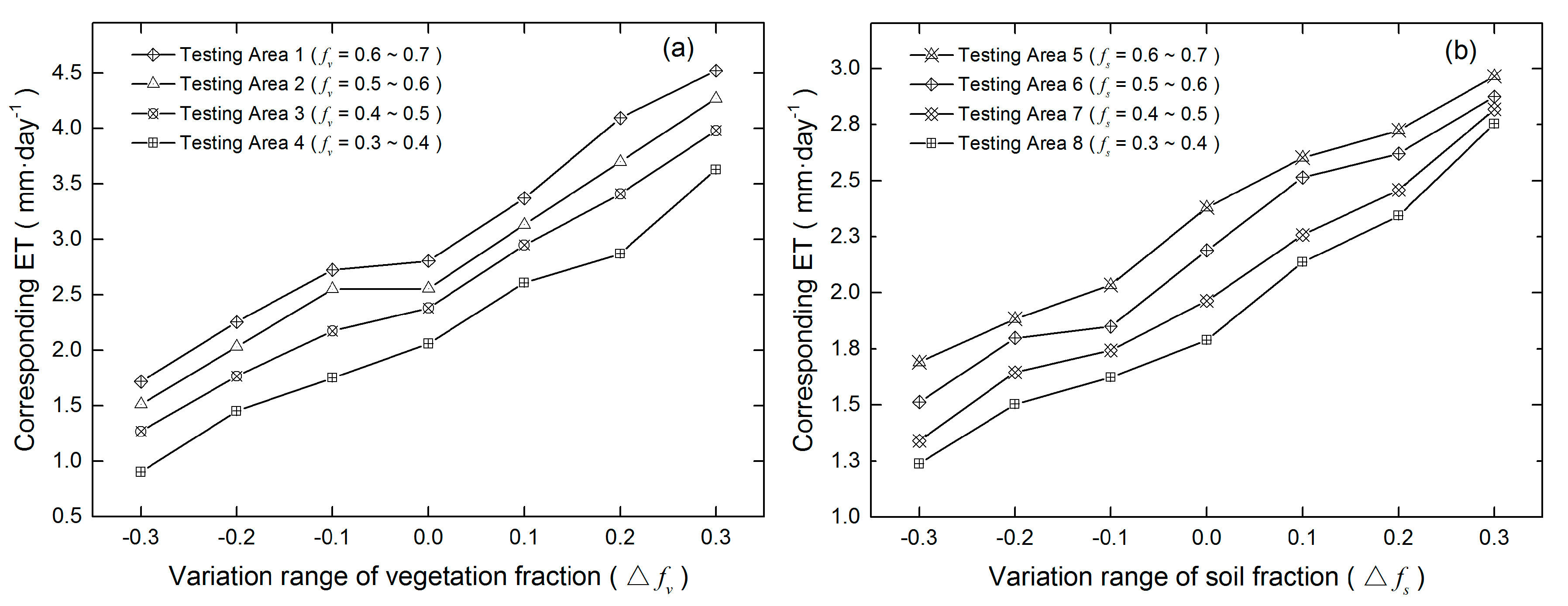
| Testing Area | ET Error for (mm·day−1) | ET Error for (mm·day−1) | |||||||
|---|---|---|---|---|---|---|---|---|---|
| or | 1 | 2 | 3 | 4 | 1 | 2 | 3 | 4 | |
| −0.3 | −1.088 | −1.043 | −1.113 | −1.156 | −0.689 | −0.676 | −0.624 | −0.552 | |
| −0.2 | −0.551 | −0.523 | −0.615 | −0.607 | −0.496 | −0.390 | −0.319 | −0.286 | |
| −0.1 | −0.081 | −0.004 | −0.207 | −0.308 | −0.345 | −0.339 | −0.221 | −0.167 | |
| 0.1 | 0.566 | 0.578 | 0.568 | 0.549 | 0.223 | 0.326 | 0.293 | 0.348 | |
| 0.2 | 1.289 | 1.145 | 1.031 | 0.811 | 0.345 | 0.432 | 0.495 | 0.554 | |
| 0.3 | 1.717 | 1.715 | 1.600 | 1.570 | 0.585 | 0.686 | 0.854 | 0.965 | |
| Accuracy Measures | Correlation Coefficient (r) | Regression Equation | R2 | Mean Relative Error (MRE) | Root Mean Square Error (RMSE) | |
|---|---|---|---|---|---|---|
| Land Cover Type | ||||||
| Vegetation | 0.8127 | 0.6577 | 8.63% | 0.1751 | ||
| Soil | 0.7153 | 0.5077 | 5.97% | 0.1522 | ||
| Impervious surface | 0.6708 | 0.4444 | 5.73% | 0.1477 | ||
| Data Type | Total | Vegetation | Soil | Impervious Surfaces | |||||
|---|---|---|---|---|---|---|---|---|---|
| Indicator | Zheng’s Model | Modified Model | Zheng’s Model | Modified Model | Zheng’s Model | Modified Model | Zheng’s Model | Modified Model | |
| () | 0.7647 | 0.7921 | 0.5914 | 0.7457 | 0.6805 | 0.7225 | 0.5053 | 0.5856 | |
| () | 0.6421 | 0.7625 | 0.8127 | 0.8669 | 0.7153 | 0.7339 | 0.6708 | 0.7253 | |
| Taylor Skill () | 0.7646 | 0.8351 | 0.6960 | 0.8574 | 0.7422 | 0.7814 | 0.5414 | 0.6561 | |
| Accuracy Measures | Correlation Coefficient (r) | Regression Equation | R2 | Mean Relative Error (MRE) | Root Mean Square Error (RMSE) | |
|---|---|---|---|---|---|---|
| Land Cover Type | ||||||
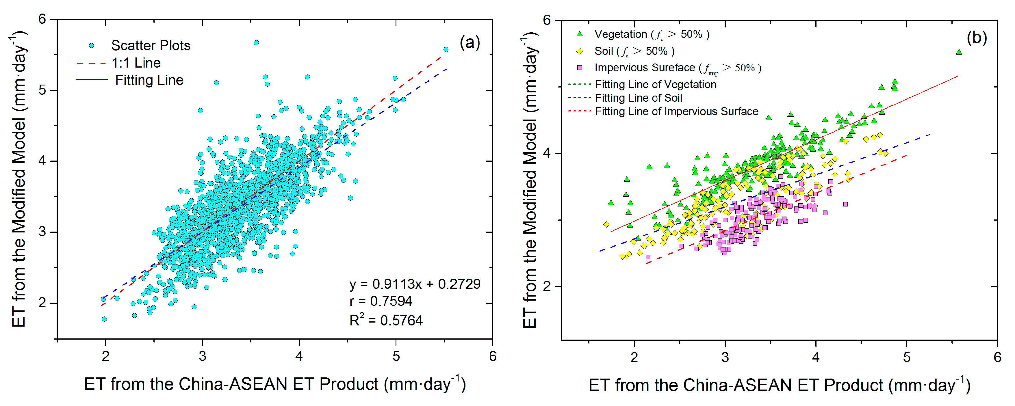
| Overall | 0.7594 | 0.5764 | 8.90% | 0.3747 | ||
| Vegetation | 0.8861 | 0.7843 | 7.80% | 0.3398 | ||
| Soil | 0.7805 | 0.6071 | 8.87% | 0.3446 | ||
| Impervious surfaces | 0.7462 | 0.5542 | 8.77% | 0.3191 | ||
© 2017 by the authors. Licensee MDPI, Basel, Switzerland. This article is an open access article distributed under the terms and conditions of the Creative Commons Attribution (CC BY) license (http://creativecommons.org/licenses/by/4.0/).
Share and Cite
Zhang, Y.; Li, L.; Chen, L.; Liao, Z.; Wang, Y.; Wang, B.; Yang, X. A Modified Multi-Source Parallel Model for Estimating Urban Surface Evapotranspiration Based on ASTER Thermal Infrared Data. Remote Sens. 2017, 9, 1029. https://doi.org/10.3390/rs9101029
Zhang Y, Li L, Chen L, Liao Z, Wang Y, Wang B, Yang X. A Modified Multi-Source Parallel Model for Estimating Urban Surface Evapotranspiration Based on ASTER Thermal Infrared Data. Remote Sensing. 2017; 9(10):1029. https://doi.org/10.3390/rs9101029
Chicago/Turabian StyleZhang, Yu, Long Li, Longqian Chen, Zhihong Liao, Yuchen Wang, Bingyi Wang, and Xiaoyan Yang. 2017. "A Modified Multi-Source Parallel Model for Estimating Urban Surface Evapotranspiration Based on ASTER Thermal Infrared Data" Remote Sensing 9, no. 10: 1029. https://doi.org/10.3390/rs9101029