Monitoring Recent Fluctuations of the Southern Pool of Lake Chad Using Multiple Remote Sensing Data: Implications for Water Balance Analysis


1
Key Laboratory of Water Cycle and Related Land Surface Processes, Chinese Academy of Sciences, Beijing 100101, China
2
Institute of Geographic Sciences and Natural Resources Research, Chinese Academy of Sciences, Beijing 100101, China
*
Author to whom correspondence should be addressed.
Remote Sens. 2017, 9(10), 1032; https://doi.org/10.3390/rs9101032
Submission received: 6 August 2017
/
Revised: 25 September 2017
/
Accepted: 28 September 2017
/
Published: 10 October 2017
Abstract
:The drought episodes in the second half of the 20th century have profoundly modified the state of Lake Chad and investigation of its variations is necessary under the new circumstances. Multiple remote sensing observations were used in this paper to study its variation in the recent 25 years. Unlike previous studies, only the southern pool of Lake Chad (SPLC) was selected as our study area, because it is the only permanent open water area after the serious lake recession in 1973–1975. Four satellite altimetry products were used for water level retrieval and 904 Landsat TM/ETM+ images were used for lake surface area extraction. Based on the water level (L) and surface area (A) retrieved (with coinciding dates), linear regression method was used to retrieve the SPLC’s L-A curve, which was then integrated to estimate water volume variations (). The results show that the SPLC has been in a relatively stable phase, with a slight increasing trend from 1992 to 2016. On annual average scale, the increase rate of water level, surface area and water volume is 0.5 cm year−1, 0.14 km2 year−1 and 0.007 km3 year−1, respectively. As for the intra-annual variations of the SPLC, the seasonal variation amplitude of water level, lake area and water volume is 1.38 m, 38.08 km2 and 2.00 km3, respectively. The scatterplots between precipitation and indicate that there is a time lag of about one to two months in the response of water volume variations to precipitation, which makes it possible for us to predict . The water balance of the SPLC is significantly different from that of the entire Lake Chad. While evaporation accounts for 96% of the lake’s total water losses, only 16% of the SPLC’s losses are consumed by evaporation, with the other 84% offset by outflow.
1. Introduction
Lake Chad, one of Africa’s largest freshwater lakes, lies in an endoreic basin on the southern margin of the Sahara Desert (Figure 1). Like most lakes located in a hydrologically closed drainage system, the fluctuation of Lake Chad is directly related to river inflow, which varies according to the annual rainfall over the basin [1,2]. The climate of the Lake Chad basin can be classified as tropical hyper-arid, with four distinct climate zones of different rainfall levels. Moving from the north to the south of the basin, the climatic zones are the Saharan climate, the Sahelo-Saharan climate, the Sahelo-Sudanian climate and the Sudano-Guinean climate, respectively. Accordingly, the annual average rainfall ranges from nearly 1600 mm in the southwest to less than 150 mm in the north [3]. As a result, approximately 90% of Lake Chad’s water comes from the Chari/Logone River system in the south of the basin, with the remaining 10% coming from local precipitation and from the El Beid and Komadougou Yobe Rivers [4,5,6,7].
As a highly variable shallow lake (less than 7 m), Lake Chad is very sensitive to precipitation and runoff changes. For example, in the 1960s, Lake Chad was the world’s sixth largest inland water body, with an open water area of 25,000 km2, but it has since shrunk dramatically to only 2000 km2 in the subsequent forty years [8]. The most striking variation of Lake Chad during this period is the recession of the lake in 1973–1975, which has been widely reported in the media [2]. As Figure 2 shows, due to a series of devastating droughts over the African Sahel belt, the open water area of Lake Chad has been separated into two individual parts by a shallow zone termed as the “Great Barrier” since 1973 [9]. Since then, Lake Chad has been composed of two basins: the southern basin of the lake, fed directly by the inflows from the Chari/Logone River (annual mean 27.14 km3 year−1 between 1960 and 2013) and the northern basin, which receives only a small contribution from the Yobe River (annual mean 0.56 km3 year−1 between 1960 and 2013). As a result, these two basins vary differently with time: the northern basin has been occasionally and partially inundated while the southern basin has remained a free water zone [2].
Bounded by four countries (Cameroon, Chad, Niger and Nigeria), Lake Chad provides a vital source of water to more than 30 million people in these riparian states [10]. The lake recession in the second half of the 20th century has triggered conflicts related to food security, poverty, and migration [11,12]. It is therefore crucial to continuously monitor Lake Chad to increase our understanding of water resource availability. Due to the lack of reliable in situ meteorological and hydrological observations, it is very challenging and costly to document the fluctuation of Lake Chad using traditional techniques. Consequently, researchers have resorted to the use of satellite gravimetry, altimetry and imagery to investigate the water resources in the Lake Chad basin. For example, Coe and Birkett [13] adopted altimetric stage measurements from the TOPEX/Poseidon satellite to estimate the height of Lake Chad. Leblanc et al. [14] retrieved and analyzed the monthly total inundated area of Lake Chad from 1986 to 2011 using METEOSAT thermal maximum composite data. The spatio-temporal characteristics of water storage change within the Lake Chad basin from 2003 to 2013 was investigated by Buma and Lee [15] using the Gravity Recovery and Climate Experiment (GRACE) and Landsat imageries. Additionally, Buma et al. [12] investigated the diverse aspects of the Lake Chad basin through a combined used of updated remotely sensed and hydrological model datasets.
These studies revealed the hydrological variations of the Lake Chad basin from different aspects, which is important for local water resource management in the light of climate change. That said, these studies, in addition to those based on remote sensing techniques, have focused mainly on monitoring either water surface area or lake level [4,13,14,16,17,18]. Although several studies have tried to reveal the water storage change of Lake Chad, they are conducted on the whole basin scale [12,19]. The water volume variation of the lake itself has seldom been investigated. Furthermore, most studies have only focused on the variation of Lake Chad as a whole to study the serious lake recession in the second half of the 20th century. Few studies have investigated the recent variations of its two basins individually [2,20]. The drought episodes in the region have profoundly modified the natural resources in the basin and around the lake [21,22,23], and a re-evaluation of Lake Chad’s water resources is necessary. Since the lake’s separation into two individual parts during 1973–1975, open water has persisted only in the southern basin, mostly near the Chari delta [2]. Therefore, our study focuses on the open water body in Lake Chad’s southern basin.
The development of sophisticated remote sensing techniques has made it possible to retrieve both water level and surface area directly from remote sensing observations. Several recent studies show that water volume variations can be estimated indirectly using the combination of satellite altimetry and imagery data [24,25,26,27]. The innovation of this research is the application to Lake Chad and the investigation of the water budget components. Accordingly, the main objectives of this paper are: (1) to provide comprehensive monitoring of the south pool of Lake Chad (SPLC) in the recent 25 years through multiple remote sensing observations, in which water level, surface area and volume variations of Lake Chad are estimated without any in situ measurements and bathymetry maps; and (2) to conduct water balance analysis to investigate different components of the lake’s water budget, based on the estimated water volume variations, river inflow observations and meteorological datasets from the Climatic Research Unit (CRU).
2. Study Area
2.1. Lake Chad Setting
Lake Chad features several types of landscape, which vary according to the water level [28,29]. Over the first half of the 20th century and up until the start of the 1970s, Lake Chad is a single body of water with limited marshy vegetation along the shores. The water surface area over this period ranges from 15,000 to 25,000 km2. Since 1973, Lake Chad has been experiencing a small lake phase with an area of about 2000–14,000 km2 [30]. Most of its areal extent is covered by permanent or seasonal marshes rather than open water. The most distinguishing feature of “Small Lake Chad” is the division of the inundation area into two separate large basins by shoals covered with dense vegetation, which are referred to the “Great Barrier”. As a result, Lake Chad in this phase is composed of several water bodies with only one permanent water pool facing the Chari delta in the southern basin [2]. Due to the small inflow of Yobe River, the northern basin has been occasionally and partially inundated since 1975. There are even observations showing that it has completely dried up on several occasions [9]. The term “Dry Small Lake Chad” proposed by Lemoalle et al. [2] is used to describe a state when the northern basin remains dry all year long.
The research of Lemoalle et al. [2] shows that Lake Chad has been functioning as a Small or Dry Small Lake since 1975. As a result, it has been a shriveled, fragmented collection of several water bodies for more than 40 years. The permanent open water pool in the southern basin was adopted as our study area in this paper, because it is the only one of several water bodies that provides reliable water resources to human, livestock and wildlife communities (Figure 2).
2.2. Climatic and Hydrologic Variability
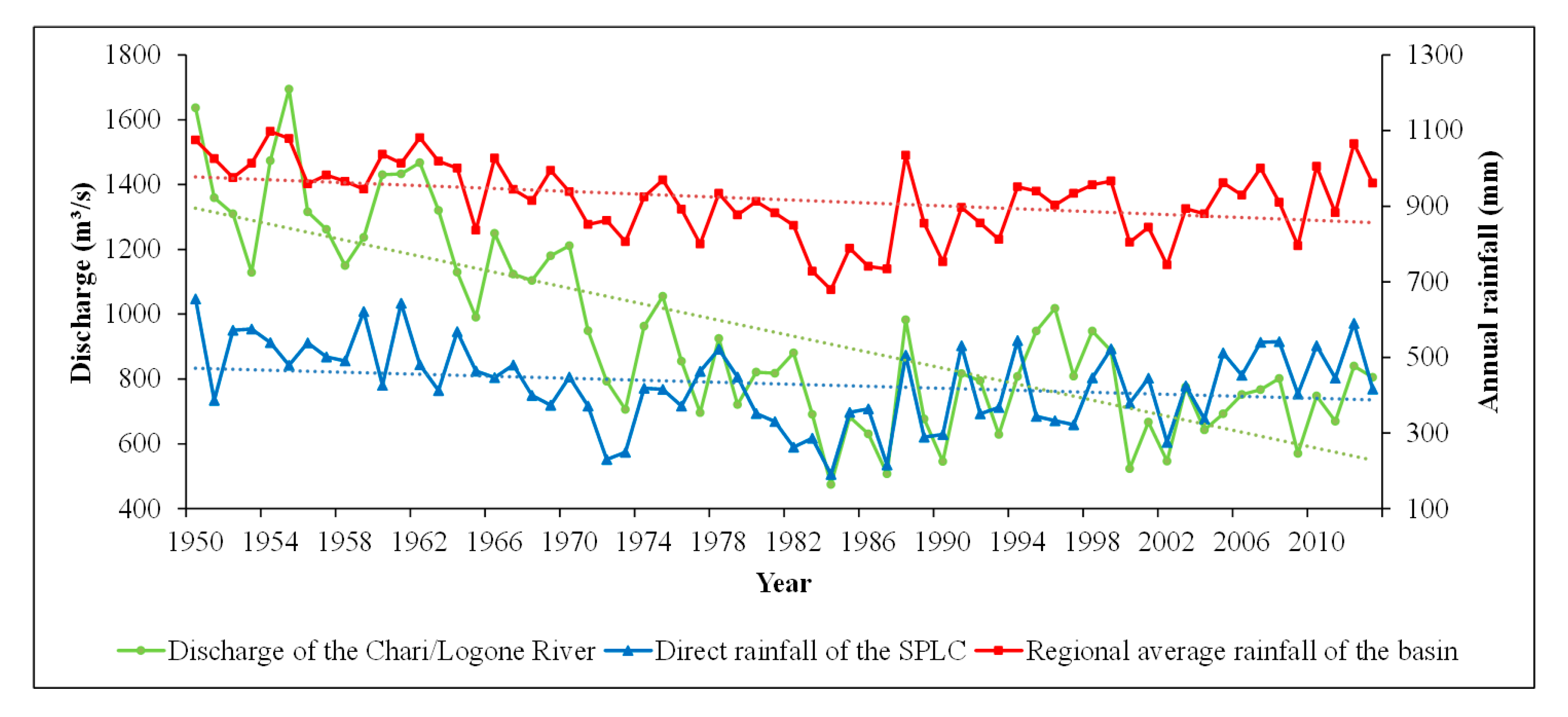
Direct rainfall and the discharge from Chari River are the only two water sources for the southern pool of Lake Chad (SPLC). Consequently, the level, volume and surface area of the lake fluctuate as a function of climatic and hydrological variations. The monthly discharge of the Chari/Logone River system at N’Djamena, the direct rainfall over SPLC, and the regional average rainfall of the whole basin are presented in Figure 3. The discharge observations are provided by the Lake Chad Basin Commission (LCBC), and the rainfall data are retrieved from the gridded climate dataset produced by the Climatic Research Unit (CRU). More details about the data source are presented in Section 3. Because of the steep south-to-north rainfall gradient, the average precipitation over the whole basin is more than twice the direct precipitation over Lake Chad. Although all previous studies have confirmed the general decreasing trend of precipitation since the 1960s, the precipitation time series can be divided into two phases by adopting the severe drought in 1984 as a turning point.
During the first period, Lake Chad’s direct precipitation decreased from 655.20 mm year−1 to 190.20 mm year−1 with an annual average rate of −7.87 mm year−1. At the basin scale, precipitation decreased from 1074.90 mm year−1 to 679.44 mm year−1, with an annual average rate of −7.40 mm year−1. In contrast, the precipitation has increased since 1985. Specifically, the annual average rate of increase over Lake Chad and the whole basin is 5.48 mm year−1 and 4.84 mm year−1, respectively. As for the discharge of the Chari/Logone River, it has decreased by almost 50% over the first 40 years, from about 43 km3 year−1 in the 1950s to about 23 km3 year−1 in the 1980s. The annual average rate of decrease is about −0.73 km3 year−1. However, due to the increase in rainfall, the variation of discharge from 1985 to 2013 shows a slightly increasing trend, with an annual average rate of 0.02 km3 year−1.
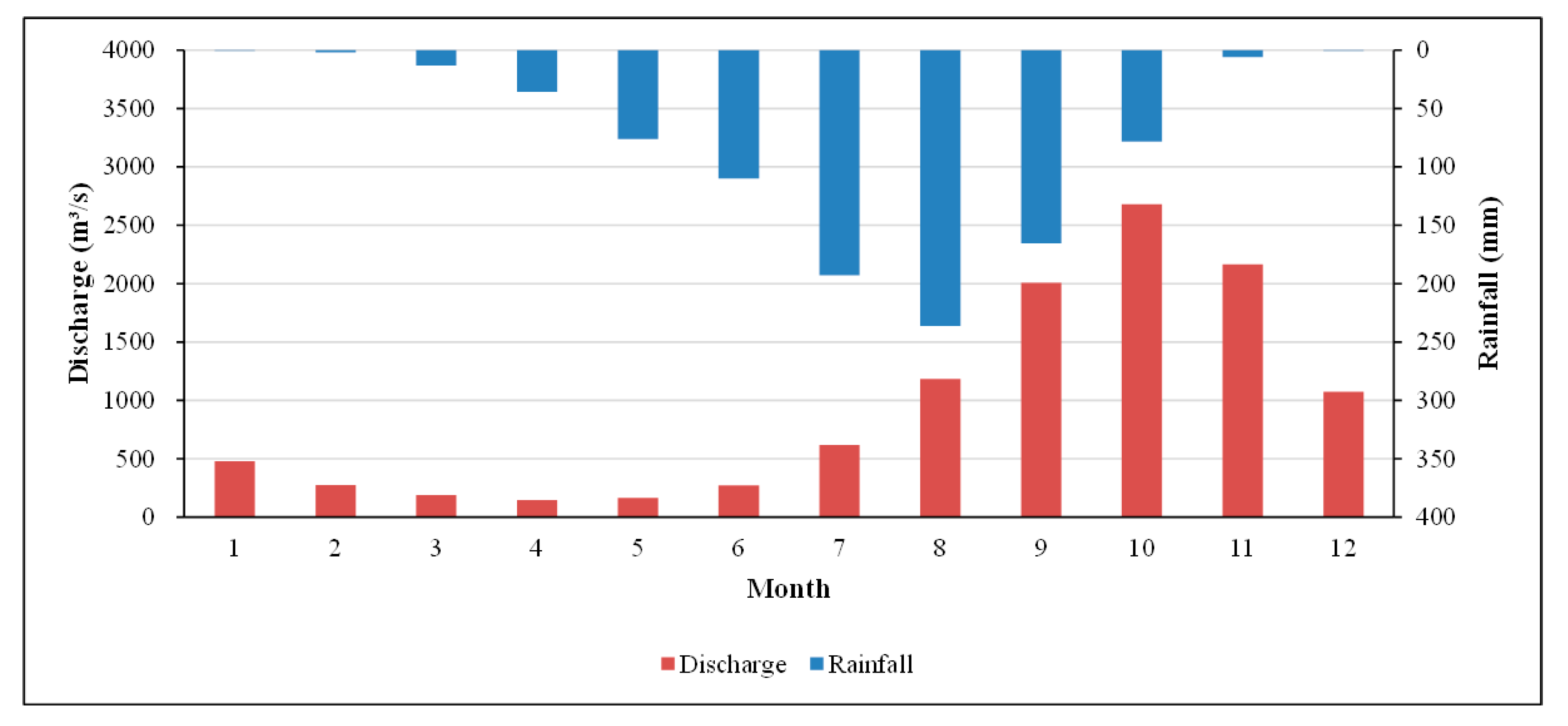
Besides significant inter-annual variation, the seasonal variation of precipitation over the study area is obvious. Lake Chad has a Sahelian climate, which is characterized by a relatively short rainy season from June to October and a long dry season for the rest of year [30]. As presented in Figure 4, the precipitation during the rainy season accounts for about 85% of the total annual precipitation. The comparison of these two curves shows that there is a time lag of about one to two months in the response of streamflow to precipitation. As a result, most of the discharge is observed from July to December with a peak value in October.
3. Data Source
3.1. Satellite Altimetry Products for Water Level
Satellite radar altimetry is a successful technique that is widely used to monitor lake level variations [25,26,27,31,32]. In this paper, four satellite altimetry products were used to monitor the fluctuations of Lake Chad.
The Global Reservoir and Lake Monitor (GRLM) product is prepared by the United States Department of Agriculture’s Foreign Agricultural Service (USDA-FAS), in cooperation with NASA and the University of Maryland. Near-real time data from multiple missions including the Jason-3, Jason-2/OSTM, Jason-1, TOPEX/POSEIDON (T/P) and ENVISAT, are utilized in this product to routinely monitor lake and reservoir height variations [33]. Relative height variations of Lake Chad from 1992 to 2016 are provided with respect to a nine-year mean level derived from T/P altimeter observations (http://www.pecad.fas.usda.gov/cropexplorer/global_reservoir/).
Hydroweb is developed by LEGOS (Laboratoire d’Etudes en Géophysique et Océanographie Spatiales) in France. Based on altimetry data from T/P, Jason-1, Jason-2, ENVISAT and GFO data, Hydroweb provides time series over water levels of about 100 lakes and 250 sites on large rivers [34]. Water level records of Lake Chad from 1992 to 2016 are available now in Hydroweb (http://hydroweb.theia-land.fr/).
The River Lake Hydrology (RLH) product developed by the European Space Agency and Montfort University is based on altimetry observations mainly from ENVISAT and Jason-2 (http://tethys.eaprs.cse.dmu.ac.uk/RiverLake/shared/main). It provides the relative water level variations of Lake Chad from 2003 to 2016 with respect to the corresponding climatological mean level, which is determined by averaging all the available water levels (referenced to the EGM96 (Earth Gravitational Model) geoid) during this period [35]. More details about the EGM96 geoid can be found in the research of Chander and Majumdar [36].
The Database for Hydrological Time Series of Inland Waters (DAHITI) is developed by the Deutsches Geodätisches Forschungsinstitut der Technischen Universität München [37]. It provides inland water level time series over lakes, rivers and reservoirs from multi-mission satellite altimetry (TOPEX, Jason-1, Jason-2, GFO, ENVISAT, Cryosat-2, and Saral/Altika). For Lake Chad, water level series with different references from 1992 to 2016 are available now in DAHITI (http://dahiti.dgfi.tum.de/en/). Within this study, ellipsoidal heights with respect to WGS84 ellipsoid have been used.
3.2. Landsat Imagery for Water Surface Area
Landsat TM/ETM+ images, because of their high spatial resolution (30 m), have been widely used to monitor the variations of water surface area [38,39,40]. In total, 904 Landsat TM/ETM+ images from 1991 to 2016 were obtained from the USGS Glovis data archive (http://glovis.usgs.gov). All images used are cloud free or have a slight cloud cover (less than 5%). Due to the post-2003 Scan Line Corrector (SLC) failure, there are wedge-shaped gaps and missing pixels in the ETM+ images acquired afterwards [41]. A simple gap-filing extension toolbox (landsat_gapfill.sav) in the ENVI (Environment for Visualizing Images) software was used to remove the gaps in the ETM+ SLC-off images. This gap-filling method is based on the local linear histogram matching technique chosen by USGS [42,43]. Following the instructions presented by Chander et al. [44], scenes were screened to remove cloud and cloud shadow and converted to Top-of-Atmosphere (TOA) reflectance based on the coefficients in the header file.
3.3. Gridded Climate Dataset
Gridded climate dataset produced by the Climatic Research Unit (CRU) is used in this paper to represent the climatic conditions of the study area. It contains interpolated average data from climatic models and stations over a spatial grid of 30 arc minutes for the period 1901–2015. A number of climatic variables (e.g., cloud cover, precipitation, temperature, vapor pressure, potential evapotranspiration, and forest day frequency) at the monthly time scale are available in the current version 4.00. More details about data interpolation and quality assessment can be found in the studies of Harris et al. [45] and Harris and Jones [46]. In this study, monthly precipitation and potential evapotranspiration from the grid cells covering Lake Chad were extracted from CRU TS Version 4.00 product using the water surface area derived from Landsat imagery.
3.4. Field Observations
In situ observations of water level and surface area would be very helpful to studies similar to ours. The research of Bouchez et al. [47] shows that the lake level of Lake Chad has been monitored non-continuously from 1956 to 2008. However, the fact is that no such observations are available for us during the period under consideration (1991–2016). Monthly discharge of the Chari/Logone River system observed at N’Djamena is used for water balance analysis. Monthly precipitation and potential evaporation observations from seven meteorological stations (Figure 1) are used to evaluate the accuracy of CRU products. All of these field observations are provided by the Lake Chad Basin Commission (LCBC) composed of Cameroon, Chad, Niger, Nigeria, Central African Republic and Libya.
4. Methodology
4.1. Water Surface Mapping
The vivid spectral information provided by Landsat TM/ETM+ images has been widely used for mapping water surface area [38,39,40]. The basic logic of these studies is to highlight the difference between water bodies and other objects through the calculation of water indexes [48]. The water index used in this research is the Modified Normalized Difference Wetness Index (MNDWI) proposed by Xu [49], which was demonstrated by previous studies to have a relatively strong performing metric compared to various water detection indexes across a range of environments [38,50,51,52]. The definition of MNDWI is given as follows:
where Green and MIR are the surface reflectance of the green band and middle infrared band (MIR) of Landsat TM/ETM+ images, respectively. Because of their high absorption in the MIR band (1.55~1.75 ) and high reflectance in the Green band (0.52~0.60 ), water features usually have high positive values. Non-water features such as soil and vegetation have low negative values because they reflect more in MIR band than in the green one. Therefore, a proper definition of specific thresholds of MNDWI classification can be used to distinguish water features from other land cover components. Following the procedure proposed by Zhu et al. [53], the water surface area of Lake Chad is extracted as follows:
- (1)
- Calculation of MNDWI. As cloud and cloud shadow have already been filtered out from the surface reflectance data, MNDWI can be calculated directly for all the Landsat images available.
- (2)
- Establishment of water mask. For each scene, all pixels with positive MNDWI values are recognized initially as water surface. However, for the whole period from 1991 to 2016, only pixels with a frequency higher than 90% were assumed as water surface. A ten-pixel buffer zone was then created over the continuous water surface and used as the water mask of our study area.
- (3)
- Definition of the MNDWI threshold. Although numerous studies have been conducted to address the threshold of water indexes, how the threshold should be defined is still far from conclusive. It seems that the proper threshold of water indexes is variable for different lakes. Following the manual adjustment procedure by Xu [49] and recommendation by Ji et al. [54], different MNDWI threshold values were tested within the water mask established above. After repeated tests and careful checks on the resulting water body boundary, the threshold value of MNDWI for Lake Chad was set as 0.20.
- (4)
- Extraction of water surface area. Applying the threshold to each Landsat image within the water mask, we obtained the aquatic surface distribution over the study area. The water surface area of the SPLC was extracted by summing up the area of the large continuous pixels identified as aquatic surface.
4.2. Processing of Water Level Products
For all of the four satellite altimetry products, water level datasets are given in the form of graphs and tables. As a result, Lake Chad’s water level can be retrieved directly from these four products. However, two issues remain to be addressed.
- (1)
- The accuracy of the altimetry products. Due to the lack of in situ water level observations, it is impossible for us to evaluate the accuracy of these altimetry products directly. In this paper, the accuracy of altimetry products is evaluated indirectly through their correlation with the water surface area extracted above. For a given lake, the relationship between water level and surface area is certain. There should be significant positive correlations between these two variables [55]. Therefore, the Pearson correlation coefficient (r) between the water level and its corresponding surface area was used here to evaluate the accuracy of different altimetry products, and is calculated as:where and are the corresponding water surface area and water level acquired on the same day, respectively.
- (2)
- The inconsistency of the altimetry products. Firstly, the water level retrieved from different altimetry products is referenced to different geoids. Secondly, both GRLM and RLH provide relative water level variations, while the water level retrieved from Hydroweb and DAHITI is presented as an absolute value. These altimetry products need to be transformed into the same reference system so that consistent comparisons can be made. In this paper, this transformation is achieved through a simple offset method, and the WGS84 ellipsoid involved in the DAHITI product is adopted as the universal reference system. Specifically, the offset is determined by averaging the differences between water levels retrieved from DAHITI and those retrieved from other altimetry products. To remove the noise of some outliers, the differences larger than three times the standard deviation have been removed. After the reference system of all altimetry products has been transformed into WGS84 ellipsoid, a direct comparison is conducted to further investigate the accuracy of different altimetry products.
4.3. Water Volume Estimation
The relationship between water level (L) and surface area (A) for a given lake is certain. Therefore, once enough water level and surface area observations are available, the L-A curve can be determined through statistical analysis [56,57]. Specifically, following the scatter diagram of water level and surface area, the L-A curve can be retrieved by either linear or nonlinear regression. Once the L-A curve is known, the water volume variations () caused by a given water level change () can be estimated as:
where is the water surface area corresponding to water level following the retrieved L-A curve. According to Duan and Bastiaanssen [25] and Tong et al. [27], the total volume () of a lake can be defined as the sum of a constant volume () and as follows.
If we define as the water volume corresponding to the lowest water level during the study period, the resulting is referred to as Water Volume Above the Lowest water Level (WVALL). Consequently, the relationship between WVALL and water level (L-V curve) can be established by defining in Equation (3) as the lowest water level. The retrieved L-V curve is the integration of the functional relationship between surface area and water level, and the estimated WVALL is the relative water volume variation for the purpose of water balance analysis, rather than an absolute value.
4.4. Lake Water Balance
The water balance of the southern pool of Lake Chad can be expressed by the following:
where and are the amount of direct precipitation and evaporation, respectively. These two components are functions of water surface area and their respective rate. is the inflow of the lake from the Chari/Logone River system. is the outflow from the lake, which includes both the discharge of the surface water to the northern basin and the seepage of the lake in the form of groundwater discharge. represents the uncertainties in the water balance arising from errors in the data and water losses due to human and animal consumption, which usually cannot be accounted for directly [58,59].
In this research, is estimated from remote sensing observations as described above. and are retrieved directly from the CRU product by using the water surface extracted from Landsat images as the mask. is the discharge of the Chari/Logone River observed at N’Djamena. Therefore, is the only unknown component to be estimated from water balance analysis. Depending on the objective, the budget equation is applied to three time scales, including daily scale between two successive dates, monthly scale and annual scale.
5. Results
5.1. Comparison of Different Altimetry Products
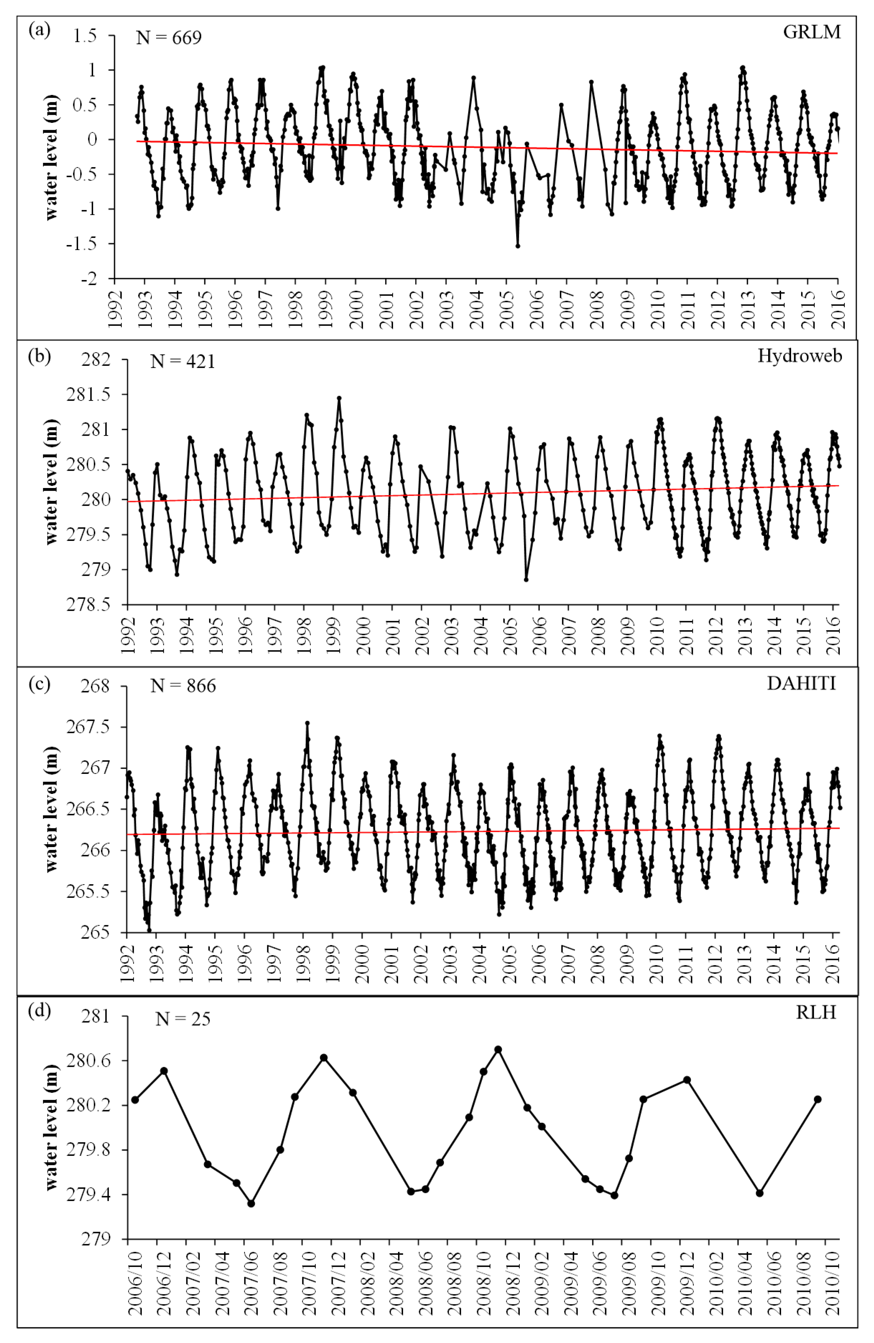
Figure 5 presents water level variations retrieved from different altimetry products and there is significant difference in the number of samples. RLH product only provide water level monitoring over a very short period. Its time period ranges from 3 October 2006 to 7 September 2010 with a sample size of 25. In contrast, long-term water level monitoring is observed in GRLM, Hydroweb and DAHITI products, all of which provide 25-year monitoring data of Lake Chad from 1992 to 2016.
Due to the lack of in situ water level observations, it is difficult to evaluate the accuracy of altimetry water level products directly. However, a close look of Figure 5 shows that the difference in the accuracy of these four products is significant. Take GRLM and Hydroweb for example: although both products provide monitoring data of Lake Chad from 1992 to 2016, they have opposing water level variation trends. Specifically, a slight downward trend is observed in the GRLM product with an annual average rate of −0.7 cm year−1, while the water level retrieved from Hydroweb indicates a slight upward trend with an annual average rate of 0.9 cm year−1. A slighter increasing trend is observed in the water levels provided by DAHITI product. The rate of increase on annual average scale is only 0.3 cm year−1. Therefore, the accuracy of the altimetry products need to be evaluated before they are used to judge the variation trend of Lake Chad.
In this paper, we used correlation analysis to evaluate the accuracy of different altimetry products. Figure 6 presents the scatterplots of the water level retrieved from altimetry products and water surface area extracted from Landsat images. Due to the small sample size of RLH, it is impossible to obtain enough samples with dates consistent with that of the Landsat observations. Consequently, only the scatterplots of GRLM, Hydroweb and DAHITI are shown here. There is significant difference in the number of points for the three datasets. The difference is mainly caused by the sample size of different altimetry products, because the number of Landsat images is constant. As presented in Figure 5, the sample size of GRLM, Hydroweb and DAHITI is 669, 421 and 866, respectively. As a result, the number of points for the three datasets in Figure 6 follows the same order.
In general, good agreement is achieved between the water levels retrieved from Hydroweb and DAHITI products and the corresponding water surface area extracted from Landsat images. The r produced is 0.70 and 0.67, respectively. However, a poor positive correlation is observed in the GRLM product with r of 0.16. A careful inspection of the GRLM product shows that this poor correlation relationship is mainly caused by the water levels retrieved from Jason-1 and TOPEX/POSEIDON (T/P). After removing these samples, the Pearson’s r obtained between the water levels retrieved from OSTM and the corresponding surface area is as high as 0.78. Besides, the GRLM product itself also presents the respective errors of each samples. The average errors of Jason-1, T/P and OSTM calculated for Lake Chad are 0.07 m, 0.06 m and 0.05 m, respectively. Based on the values of r and errors, it is reasonable to conclude that the accuracy of OSTM is highest among these three datasets. Therefore, only the OSTM dataset of the GRLM time series was used in this study.
5.2. Water Level Variations
Considering the limited samples of the RLH product and the relatively low accuracy of the Jason-1 and T/P datasets within GRLM, only the Hydroweb (1992–2016), DAHITI (1992–2016) and GRLM/OSTM dataset (2008–2016) were used to monitor the water level variations of Lake Chad. However, as presented in Figure 5, the water levels provided by Hydroweb and DAHITI are based on different reference surfaces, and GRLM/OSTM provides relative water level rather than absolute water level. Therefore, it is necessary to conduct consistency processing. A simple offset method was used here to transform all altimetry products into the WGS84 ellipsoid of the DAHITI product. Figure 7 presents the scatterplots of the water levels retrieved from Hydroweb and GRLM and the corresponding water levels retrieved from DAHITI. In general, there is good agreement of water levels retrieved from different altimetry products. The correlation coefficient r is as high as 0.98. The offset obtained for Hydroweb and GRLM is −13.77 m and 266.42 m, respectively.
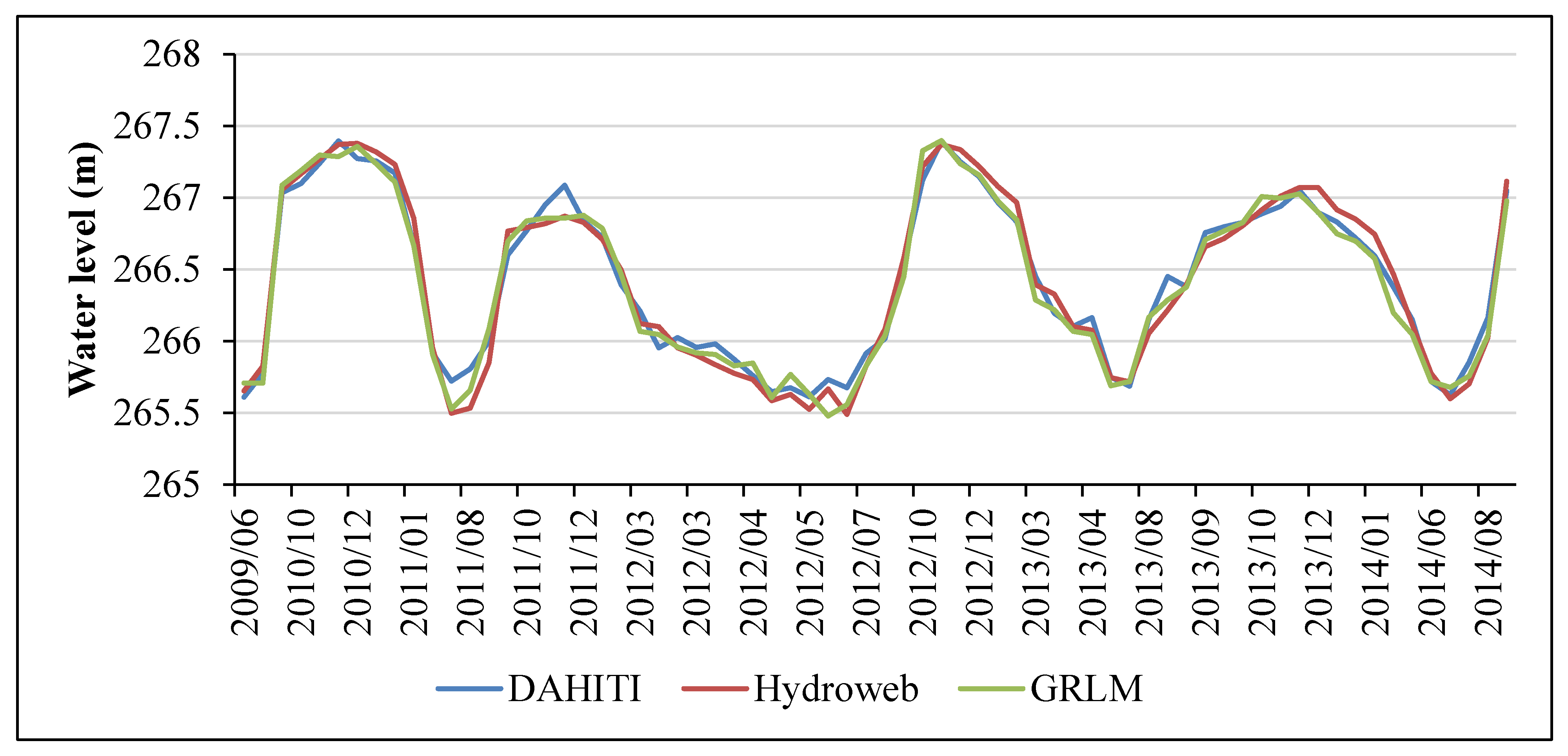
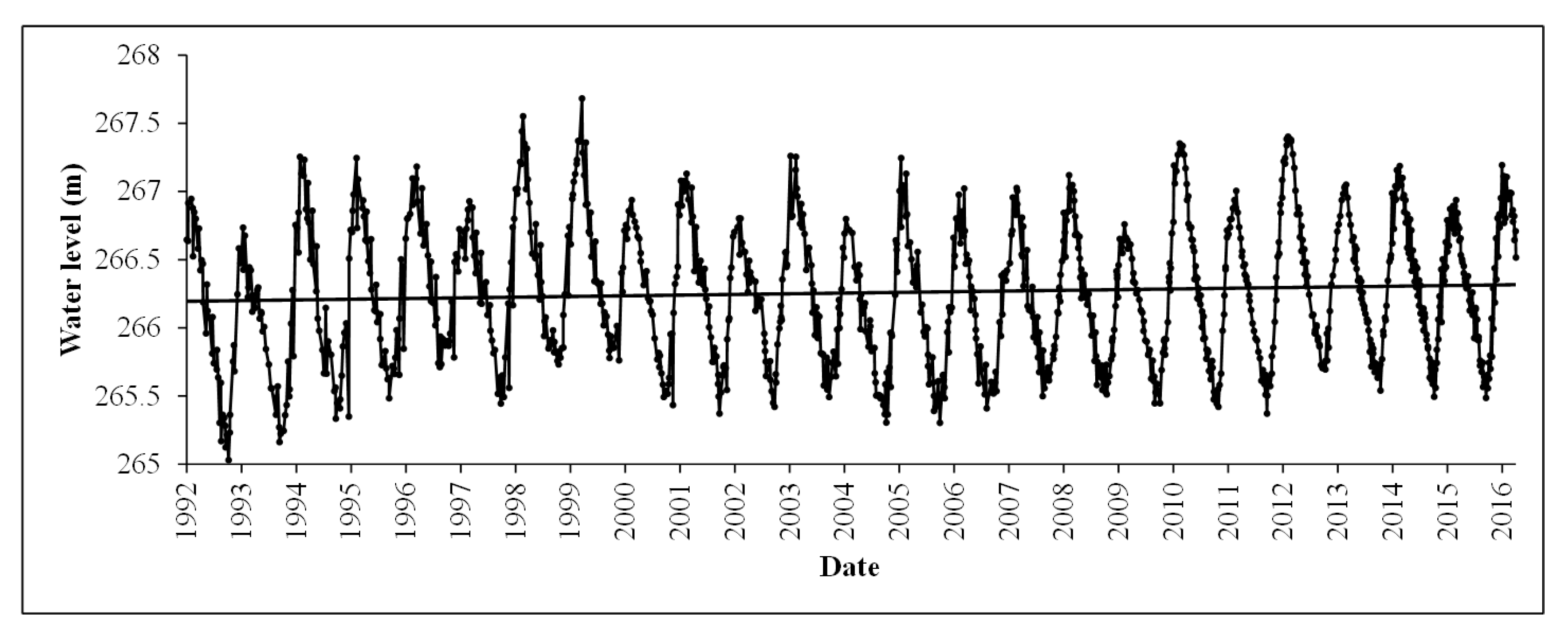
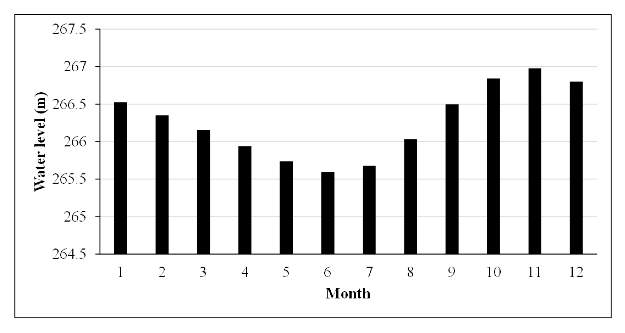
Adding the above offset to the original water levels retrieved from Hydroweb and GRLM, we obtained water level observations with the same reference as those provided by DAHITI. As a result, it is possible for us to conduct a direct comparison of different altimetry products. Figure 8 shows the time series of water level on days when the observations of all the three products are available. The water level retrieved from different altimetry products agrees well with each other with r as high as 0.99. The increase of r from 0.98 in Figure 7 to 0.99 in Figure 8 is caused by the number of samples. Judging from the magnitude of errors, the mean absolute error (MAE) and root mean square error (RMSE) are 7.86 cm and 9.82 cm, respectively. It is reasonable because the accuracy of satellite altimetry for lake level monitoring is generally reported to be better than 10 cm [60]. Figure 9 shows the time series of water levels retrieved from the combination of GRLM/OSTM, DAHITI and Hydroweb with the WGS84 ellipsoid. During the combination, when two or more samples are available on the same day, the mean values of these samples are used to represent the water level of that day. Figure 10 presents the mean monthly water level retrieved from Figure 9. Controlled by the precipitation and river inflow presented in Figure 4, the water level of Lake Chad demonstrates significant seasonal variation. It increases gradually from July to November, and then decreases from November to June of the following year. The amplitude of variation is about 1.38 meter on an annual average scale. According to Figure 9, the inter-annual variations of water level in recent 25 years show a slight increasing trend, which is opposite to the significant recession trend in the second half of the 20th century. The annual average rate of increase is only about 0.5 cm year−1. The low rate of increase indicates that Lake Chad has been in a relatively stable phase over the past 25 years.
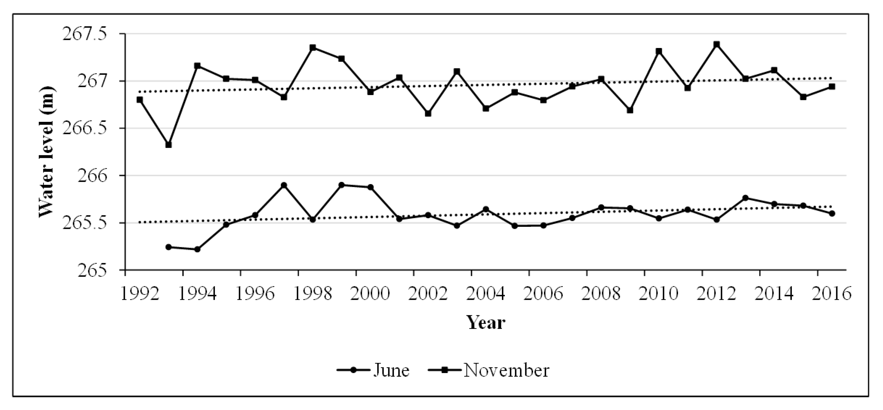
It should be noted that the number of samples presented in Figure 9 varies with time. As a result, there are some missing values in individual months. To investigate the variations in extreme water levels and eliminate the noise caused by sample size, Figure 11 presents the time series of water levels observed in June and November. These two time series confirm the upward trend of Lake Chad’s water levels, although the rate of increase is different. Specifically, the increasing rate of the low water level and high level of Lake Chad is 0.7 cm year−1 and 0.6 cm year−1, respectively. The lack of in situ water level observations makes it impossible for us to investigate the errors and uncertainties involved in Figure 9 and Figure 11. However, considering the consistent increasing trend presented in these two figures, it is reasonable to conclude that the southern pool of Lake Chad has stopped shrinking since the 1990s.
5.3. Lake Surface Area Variations
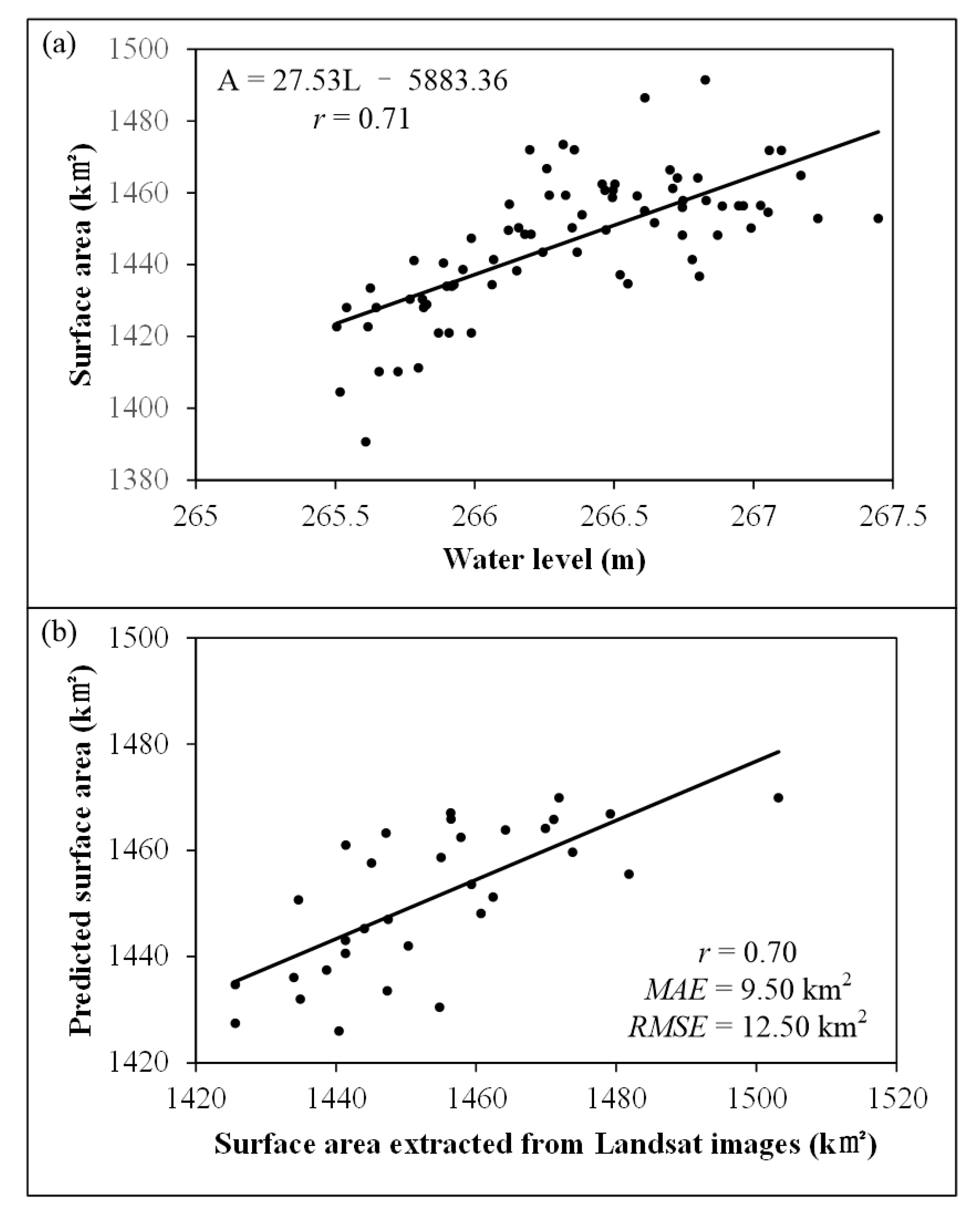
The estimation of water volume variations is based on the relationship between water surface area () and water level (). To cover the variation range of water level as much as possible, all the black points of the three altimetry products presented in Figure 6 are used. The Landsat images are acquired on the same day as the altimetry water level observations. In total, there are 110 pairs of data satisfying this criterion. However, due to the lack of in situ measurements for validation, only 77 pairs of data (70% of the sample size) were used to establish the relationship. The other 33 pairs, selected by the equidistant sampling method after all the 110 pairs were sorted by water level, were used to verify the performance of the established relationship. The results are presented in Figure 12. Nonlinear regression methods were also used in the retrieval of the L-A curve, such as the quadratic polynomial relationship proposed by Duan and Bastiaanssen [25] and Tong et al. [27], but no significant improvement was observed. Therefore, a simple linear regression model with r of 0.71 was used in this paper to describe the L-A curve of Lake Chad. In the validation process, the lake surface area estimated from the linear regression model was compared with that extracted from the Landsat TM/ETM+ images. In general, the surface area derived from the L-A curve agrees well with that retrieved from Landsat images with r as high as 0.70. The MAE and RMSE are 9.50 km2 and 12.50 km2, respectively.
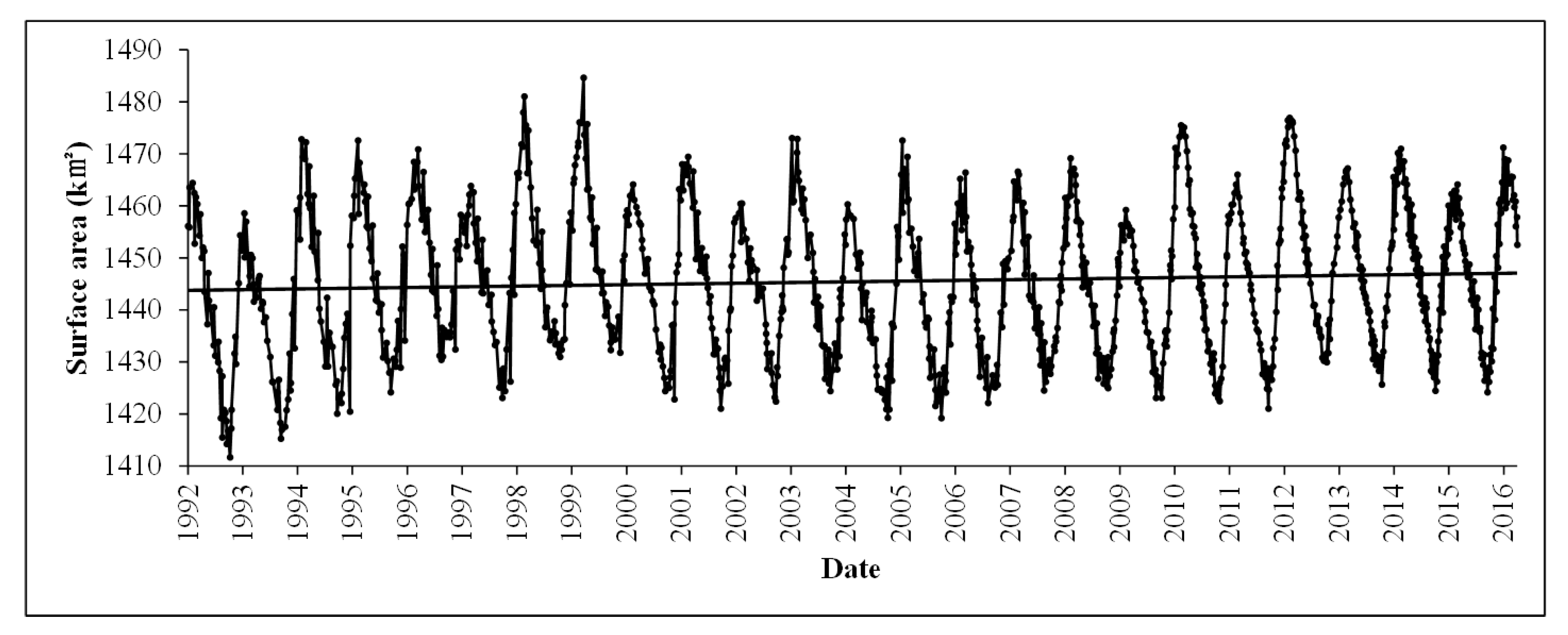
The retrieval of the L-A curve makes it possible for us to estimate lake surface area as long as water level data are available. The retrieved time-series of the lake surface area from 1992 to 2016 are shown in Figure 13. In general, the variations of lake surface area indicate a slight increasing trend with an annual average rate of about 0.14 km2 year−1. That means the southern pool of Lake Chad has increased by 3.4 km2 over the past 25 years. However, it should be noted that the MAE of the retrieved L-A curve is 9.50 km2. Therefore, the low rate of increase shows that the surface area of the SPLC has been relatively stable in recent 25 years, with an annual average surface area of 1446 km2.
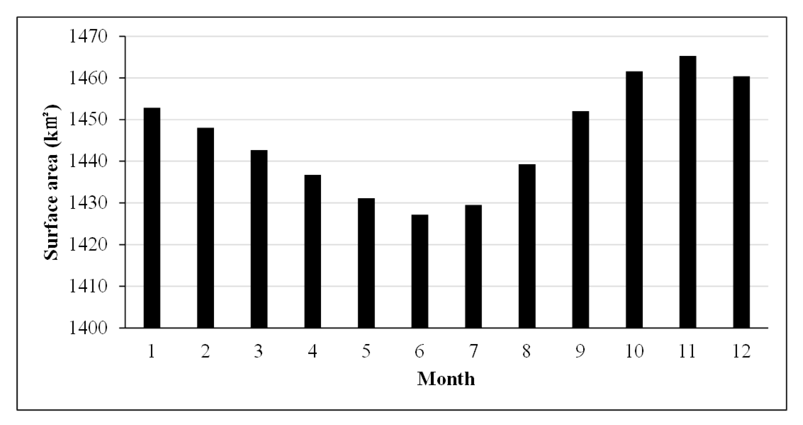
Figure 14 presents the seasonal variations of water surface area on annual average scale. It is clear that seasonal variation of the lake surface area coincides with the rainy season, with the largest surface area of 1465 km2 in November and the smallest surface area of 1427 km2 in June. The amplitude of intra-annual variation is about 38.08 km2. To further investigate the intra-annual variation of each year, Figure 15 shows the time series of lake surface area observed in June and November, which are used to represent the smallest and largest water area during a year, respectively. Consistent with Figure 11, the slight increasing trend is observed in both of these two time series. The annual average rate of increase in June and November is 0.19 km2 year−1 and 0.17 km2 year−1, respectively.
5.4. Water Volume Variations
Based on the L-A curve retrieved in Figure 12, the water volume variation of the SPLC was estimated by integration. The function is described as follows:
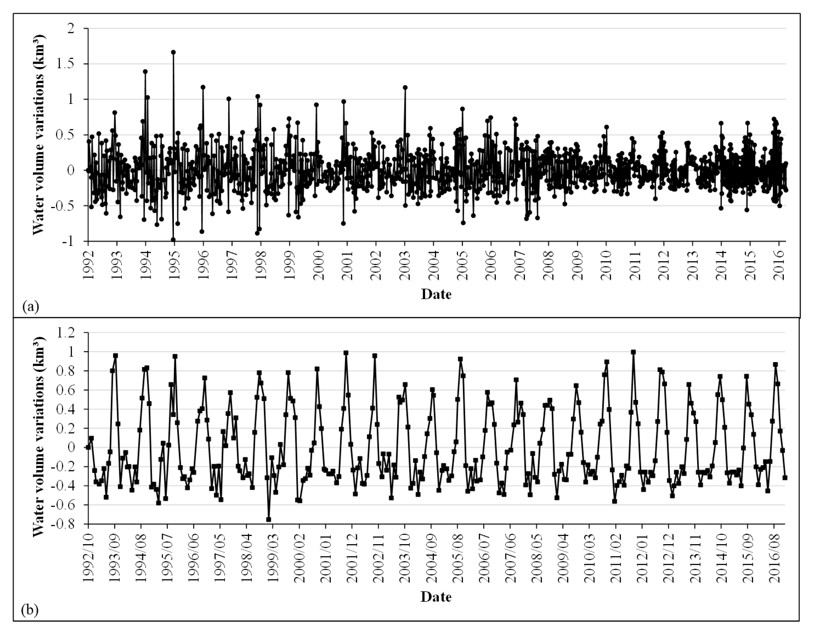
where is the water volume variation (km3) caused by the water level (m) change defined as (). Applying the function to all water levels present in Figure 9, we obtained the water volume variations of the SPLC between two adjacent water levels from 1992 to 2016. The results are shown in Figure 16a. However, because the sample size of each year varies with time, it is difficult to evaluate the water volume variations on a daily scale. For example, due to the limited number of samples prior to 2008, the time interval between two adjacent samples is much larger than that observed afterwards. As a result, the water volume variations are much more significant. To eliminate the noise caused by sample size, we applied the function to monthly scale. The results are presented in Figure 16b. Based on Figure 16, we also obtained the monthly distribution of water volume variations on annual average scale (Figure 17).
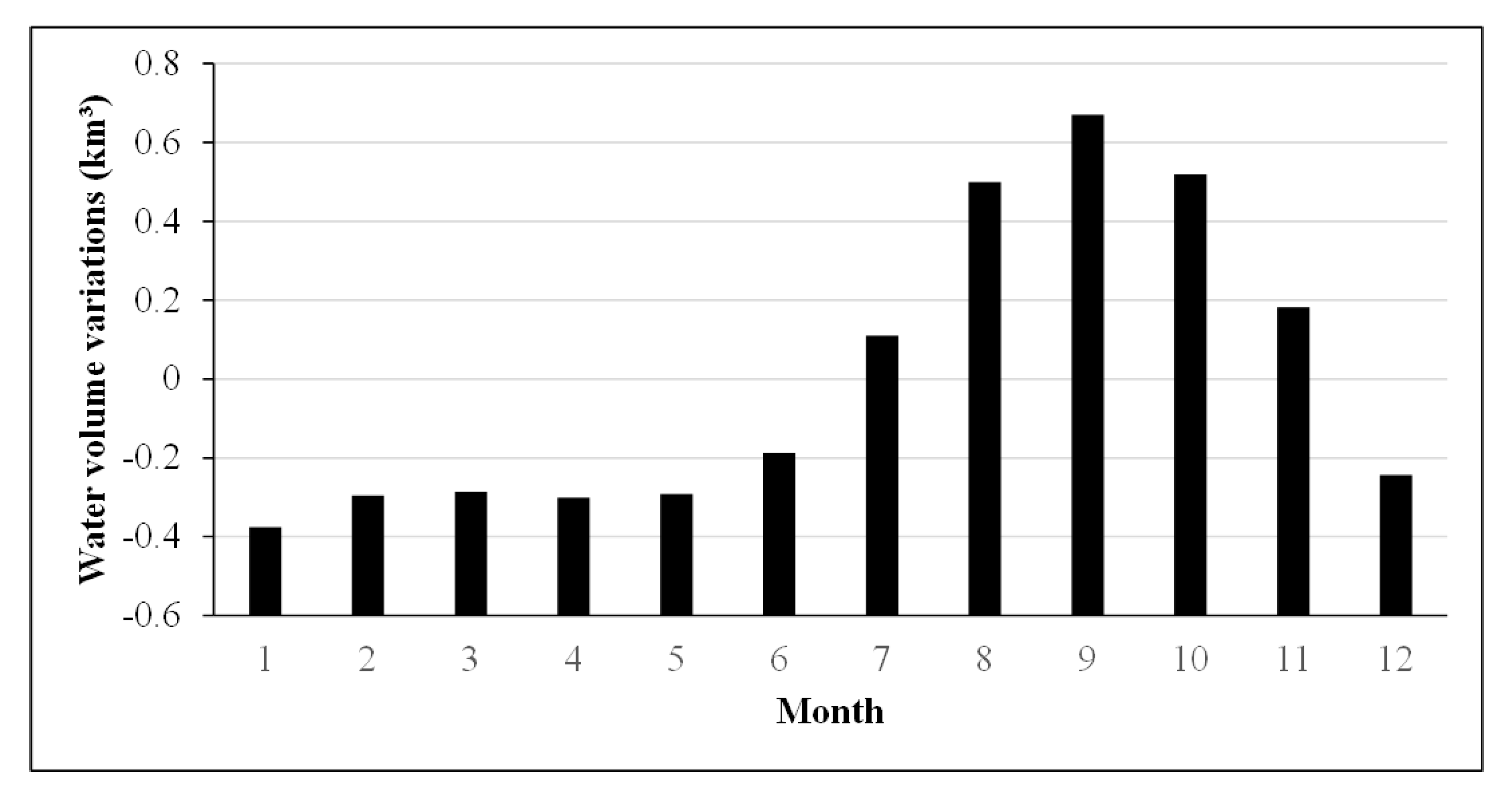
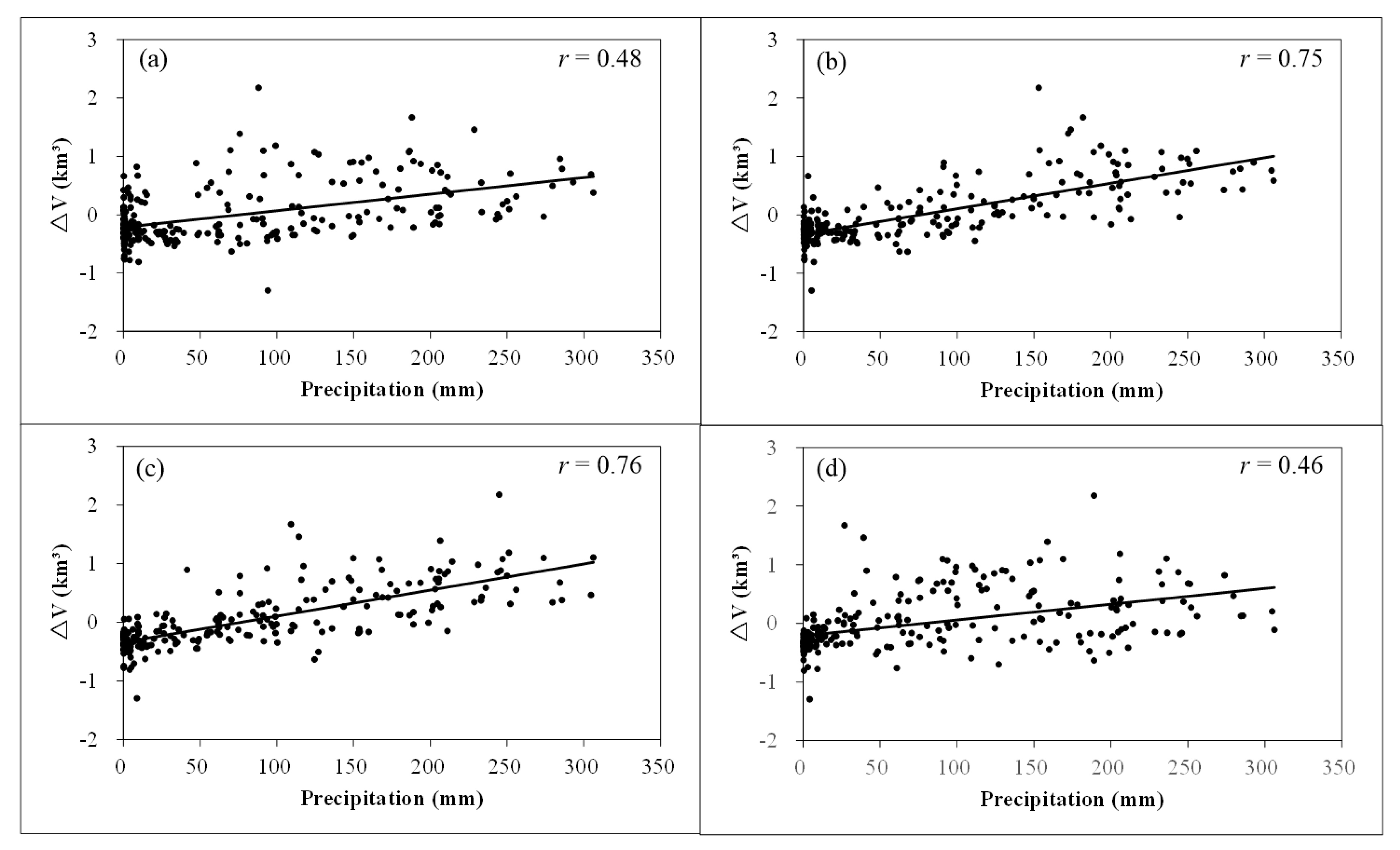
With the exception of individual months, the results effectively captured the seasonal variation of water volume. During the rainy season from July to November, the water volume of Lake Chad increases with positive values, while the negative values from December to June of the following year indicate that the water volume decreases during the dry season. On annual average scale, the water volume of Lake Chad increases most quickly in September with a rate of 0.67 km3 per month, and decreases most significantly in January with a rate of 0.38 km3 per month. To further investigate the relationship between and precipitation, the scatterplots of monthly and precipitation are presented in Figure 18. The results show that monthly water volume variations are mostly correlated with the precipitation of the previous two months, with r as high as 0.75. Therefore, there is a time lag of about one to two months in the response of water volume variations to precipitation, which means that can be predicted in advance. Linear regression method was used here to make the prediction. Seventy percent of the total 246 samples were used for calibration, and the other 30% were used for validation. The linear regression model established is described as follows:
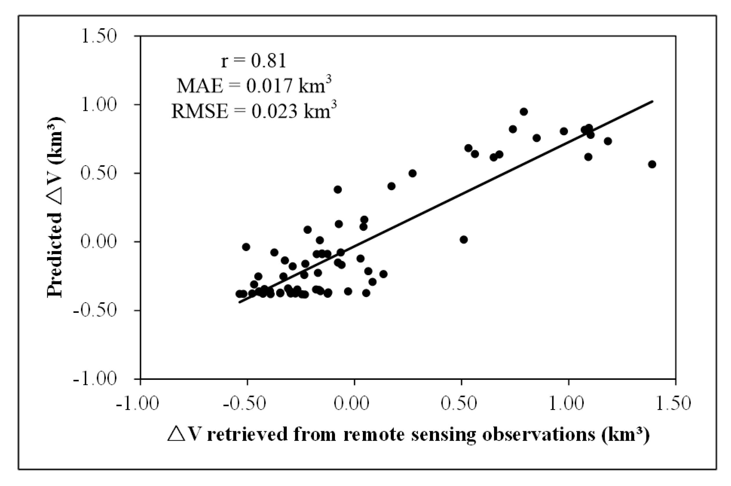
where is the monthly water volume variation (km3) to be predicted. and are the average precipitation (mm) of the Chari/Logone River basin of the previous two months, respectively. The validation results presented in Figure 19 shows that the estimated from the regression model agrees well with that retrieved from Equation (6), with r as high as 0.81. The MAE and RMSE produced are 0.017 km3 and 0.023 km3, respectively.
In Section 4.3, if in Equation (3) is defined as the lowest water level during the study period, the resulting is referred to as Water Volume Above the Lowest water Level (WVALL). The time series presented in Figure 9 shows that the lowest water level from 1992 to 2016 is observed on 7 July 1993 with a value of 265.03. As a result, the L-V curve of the southern pool of Lake Chad is defined as follows:
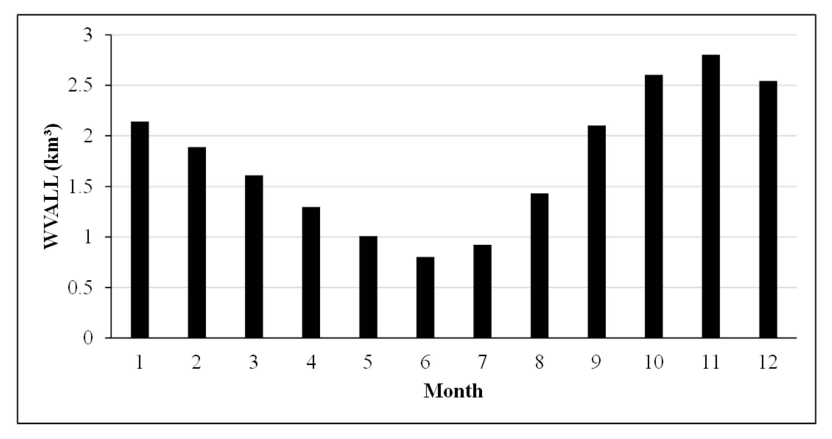
The time series of the WVALL retrieved from the L-V curve is presented in Figure 20. Because WVALL is retrieved using water level as an input, its variation trend is basically the same as that presented in Figure 9. The water volume of the SPLC has been relatively stable in the recent 25 years with respect to inter-annual variation. The annual average WVALL from 1992 to 2016 is 1.76 km3 with a small increase rate of 0.007 km3 year−1. However, the intra-annual variation of WVALL is very significant (Figure 21). On annual average scale, the amplitude of seasonal variation is as high as 2.00 km3, with the largest WVALL in November and the smallest WVALL in June.
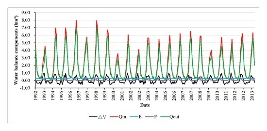
5.5. Water Balance of the LAKE
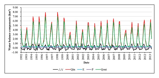
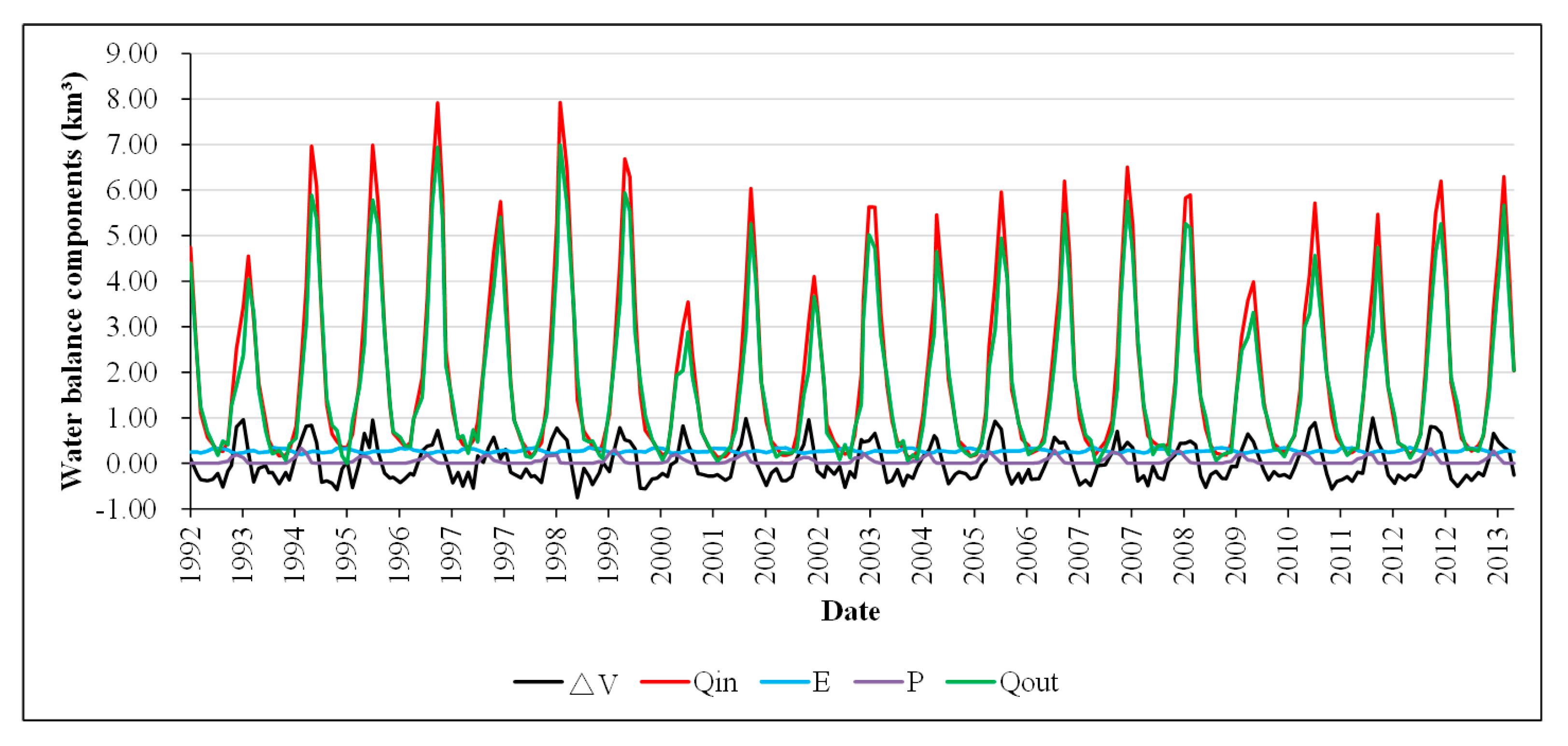
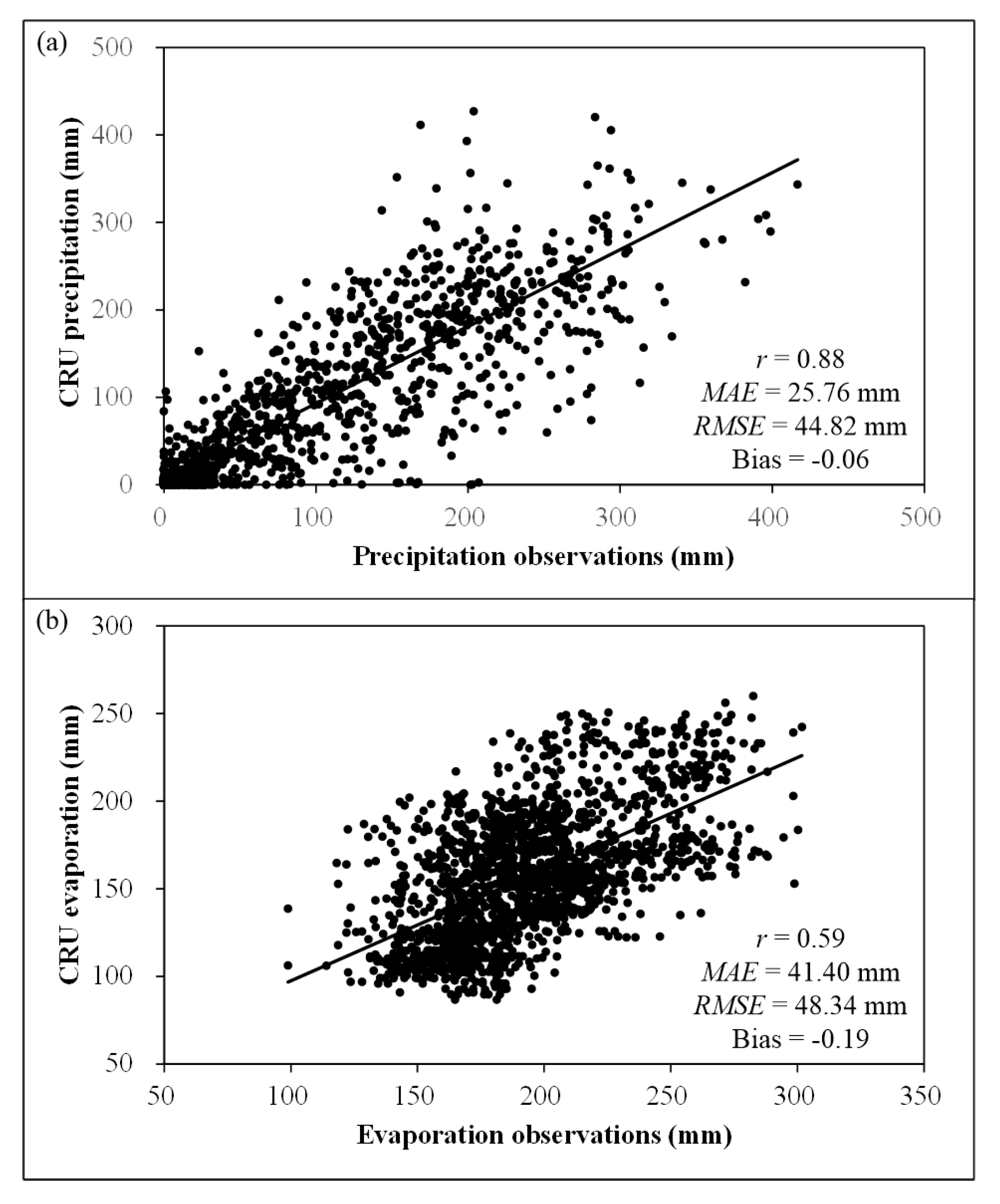
The water budget was calculated with Equation (5) using the direct precipitation and evaporation retrieved from the CRU product, lake inflow from the Chari/Logone River, and water volume variation retrieved in Section 5.4. Because values from the CRU product and discharge observations are at monthly scale, the components of the lake’s water budget presented in Figure 22 are also at monthly scale. To evaluate the accuracy of CRU product, Figure 23 presents the scatterplots of precipitation and evaporation observations versus those retrieved from CRU product. The definition of the bias (B) is defined as follows:
where and are the variables retrieved from meteorological stations and CRU product, respectively. It is obvious that the bias used here is a statistical indicator reflecting relative error. The precipitation retrieved from CRU product agrees well with observations with r as high as 0.88. The MAE and RMSE are 25.76 mm and 44.82 mm, respectively. In contrast, the Pearson’s r for evaporation is only 0.59. The high values of MAE and RMSE also indicate that there is large errors in evaporation estimates. The negative values of bias show that both precipitation and evaporation are underestimated by the CRU product. Specifically, the bias of precipitation is only −0.06 while the bias of evaporation is as high as −0.19. Consequently, it is necessary to calibrate the CRU product before it is used to investigate the water balance of Lake Chad. Here, the calibration is conducted by using the bias correction method. All the precipitation and evaporation presented in Figure 22 are corrected using their original values divided by .
Table 1 shows the monthly average of the five components of the water balance over the past 25 years. Considering the small values of on annual average scale, precipitation and river inputs of Lake Chad are basically consumed by evaporation and outflow. Specifically, the main input of the southern pool of Lake Chad is the inflow from the Chari/Logone River. The annual average discharge is 23.91 km3 year−1, which accounts for 97% of total input. The remaining 3% is supplemented by direct precipitation with an annual average of 0.67 km3 year−1. The losses result mainly from the surface and underground water discharge (84%) and evaporation (16%). The annual average losses caused by outflow and evaporation are 20.54 km3 year−1 and 4.03 km3 year−1, respectively. However, it should be noted that these two components have significant seasonal variation. Evaporation accounts for the bigger share of water losses from March to May. The contribution of outflow during these three months ranges only from 30% to 40%.
6. Discussion
6.1. Evaluating the Water Budget of the SPLC within the Whole Lake Chad Domain
The water budget of Lake Chad has been studied by a number of authors [3,30,61,62,63,64], but most of them focused on the water budget of the entire Lake Chad. Table 2 presents the summary of these previous studies. Lake Chad in the first three studies is in medium state. Only the fourth study is conducted to investigate the water budget of the Small Lake Chad. Therefore, the results of our research are compared with those observed from 1988 to 2010 by LCBC [30]. The comparison shows that there is a significant difference in the water budget components. This difference is partly caused by the selection of the study area. For example, both precipitation and evaporation are functions of the water surface area and their respective rates. The study domain of previous research is the whole of Lake Chad, while our research is focused on the permanent open water in the southern pool. According to Odada et al. [3], the open water of Lake Chad only accounts for one-third of its total area. It explains well why the amount of precipitation during 1988–2013 in LCBC [30] is three times as much as that of our research. No significant difference is observed in the amount of , because in both of these studies is taken from in situ observations.
The most distinct difference is the ratio of and to total water losses. Specifically, total water losses of these two studies are generally the same, which are 23.60 km3 year−1 and 24.57 km3 year−1, respectively. The results of LCBC [30] show that 96% of the water losses are consumed by evaporation. The research of Bouchez et al. [47] indicates that the outflow of the whole Lake Chad through infiltration represents around 10% of the total water losses. However, in our research, evaporation only accounts for 16%, with the other 84% offset by outflow. The difference in the source of water losses is explained as follows. The research of Leblanc et al. [14] indicates that most of the Small Lake Chad is covered by permanent or seasonal marshes rather than open water, which for our purposes we distinguish as “non-water area”, in contrast with the permanent open water area. According to LCBC [30], the discharge of the Chari/Logone River accounts for 96% of the total lake inflow from 1988 to 2010. It means that the inflow from other small tributaries such as El Beid and Komadugu Yobe is only 1.00 km3 year−1. Except for the precipitation falling directly on the lake surface, the amount of precipitation over the non-water area of Lake Chad is 1.23 km3 year−1. Therefore, the sum of and over the non-water area is 2.23 km3 year−1. However, the total water losses caused by and over the non-water area is 19.57 km3 year−1. There is a gap of 17.34 km3 year−1 in water losses to make up. It explains why the outflow of the southern pool of Lake Chad is as high as 20.54 km3 year−1.
In summary, although the water balance of the entire Lake Chad has been reported in several studies, the water balance of the southern pool of Lake Chad is significantly different. The water losses of the SPLC are mainly caused by outflow in the form of net surface and underground water discharge with an annual average of 20.54 km3 year−1. This outflow provides the main water source of evaporation for the whole of Lake Chad.
6.2. Evaluating Present Research in Light of Previous Work
The use of multiple remote sensing data for water volume estimation has been applied to different lakes worldwide [24,25,26,27,53,65]. For example, the water volume variations of three lakes (Lake Mead in the U.S.A., Lake Tana in Ethiopia, and Lake IJsell in Netherlands) were estimated by Duan and Bastiaanssen [25] using four satellite altimetry databases and Landsat images. The results show that estimated water volumes agree welll with in situ measurements with R2 ranging from 0.95 to 0.99 and the RMSE within 1.6% to 13.1% of the mean volumes of in situ measurements. Based on ICESat (Ice, Cloud, and Elevation Satellite) altimetry data and MODIS (Moderate Resolution Imaging Spectroradiometer) images, the water volume variations of Lake Qinghai in China were monitored in our previous research [53]. The RMSE produced is 0.5 km3, which accounts for about 0.7% of the observed total water volume variations. In general, the framework of these previous studies as well as this research is basically the same as each other. Firstly, water level and surface area are retrieved from satellite altimetry and imagery, respectively. Subsequently, the water volume variations are estimated through integration of the functional relationship between surface area and water level. The difference lies in the specific satellite altimetry and imagery product and the method used to retrieve the functional relationship between surface area and water level. In our research, four altimetry products were used to make sure that the time series of water level are as long as possible. As for the method used for the retrieval of the L-A curve, it is generally conducted based on statistical analysis [65]. The statistical model used can be either linear [26,53] or nonlinear [25,27]. Both linear and nonlinear models have been tried in this research, but no significant difference is observed in the model performance. Consequently, linear regression model is adopted because of its simplicity. In the research of Duan and Bastiaanssen [25] and Tong et al. [27], only the Water Volume Above the Lowest water Level (WVALL) was estimated by selecting the lowest water level during the study period. In contrast, as presented in Equation (6) and Figure 16, the empirical model established in our research makes it possible for us to estimate water volume variations caused by any water level change. Consequently, compared with Equation (4) recommendation by Duan and Bastiaanssen [25] and Tong et al. [27], Equation (3) proposed in this paper is more universal for monitoring the variations of water volume. The major drawback of this research is the uncertainties involved in the estimation of water volume variations. In most previous studies [24,25,26,27,53], the water level and surface area retrieved from remote sensing data are usually calibrated and validated based on in situ observations before they are used for the retrieval of the L-A curve. Besides, the estimated water volumes are also validated based on in situ observations so that the statistical method used can be adjusted and calibrated. In this research, however, due to the lack of in situ observations, it is impossible for us to evaluate directly the accuracy of water level, surface area and water volume retrieved from remote sensing data. Instead, their accuracy is evaluated indirectly. Specifically, the accuracy of water level and surface area is investigated through cross validation using correlation analysis. The validity of water volume variations is assessed through water balance analysis. Therefore, the results presented in this paper contain uncertainties arising from errors in the remote sensing data and linear regression model. The availability of reliable in situ measurements would be indispensable for future research.
7. Conclusions
Due to a series of devastating droughts, Lake Chad has shrunk dramatically in the second half of the 20th century. As a result, its open water area has been separated into two individual parts since 1973, with the water pool facing the Chari delta in the southern basin as the only permanent water area. In this paper, the variation of the southern pool of Lake Chad (SPLC) in the recent 25 years was investigated comprehensively using multiple remote sensing observations.
Four satellite altimetry products, GRLM, Hydroweb, RLH and DAHITI, were used to retrieve water level. Water surface area of the SPLC was extracted from 904 Landsat TM/ETM+ images. Because of the lack of in situ observations, the accuracy of the altimetry products was evaluated by correlation analysis, and only water levels correlating significantly with the extracted lake surface area were adopted. As a result, the Hydroweb, DAHITI and GRLM/OSTM dataset were used in this paper to monitor the water level variations of Lake Chad from 1992 to 2016. Based on the water levels retrieved above and the lake surface area extracted from Landsat images, the relationship between water level (L) and surface area (A) for the southern pool of Lake Chad was established through linear regression method. The retrieval of the L-A curve makes it possible for us to estimate lake surface area as long as water level data are available. Finally, the water volume variations were estimated through integration of the functional relationship between surface area and water level, and the water balance equation was established to investigate the components of the lake’s water budget.
The results show that Lake Chad has stopped shrinking since the 1990s. It has been in a relatively stable phase in the recent 25 years with a slight increasing trend. On annual average scale, the increase rate of water level, surface area and water volume is 0.5 cm year−1, 0.14 km2 year−1 and 0.007 km3 year−1, respectively. As for the intra-annual variations of the SPLC, it increases gradually from July to November, and then deceases from November to June of the following year. The seasonal variation amplitude of water level, lake area and water volume is 1.38 m, 38.08 km2 and 2.00 km3, respectively. The discharge of the Chari/Logone River and direct precipitation account for 97% and 3% of the SPLC’s total inputs respectively. The water losses result mainly from outflow (20.54 km3 year−1) and evaporation (4.03 km3 year−1). The outflow of the southern pool of Lake Chad provides the main water source of evaporation for the whole of Lake Chad. However, it should be noted that the outflow in this paper was estimated as the residual of the water balance equation. It contains uncertainties arising from errors in the data and water losses due to human and animal consumption. The availability of reliable in situ measurements would be indispensable for future research.
Acknowledgments
This research was funded by the National Key Research and Development Program of China (2016YFC0401307) and PowerChina International Limited. Thanks are given to the National Aeronautics and Space Administration (NASA), the Climatic Research Unit (CRU), the Lake Chad Basin Commission (LCBC), and the relevant personnel of the four satellite altimetry products (GRLM, Hydroweb, RLH and DAHITI) for their data support. Finally, we acknowledge the anonymous reviewers for their constructive comments.
Author Contributions
Wenbin Zhu designed the research, processed the remote sensing data and wrote the main part of the manuscript. Shaofeng Jia supervised the scientific development of the research project and Jiabao Yan contributed to data analysis.
Conflicts of Interest
The authors declare no conflict of interest.
References
- Coe, M.T.; Foley, J.A. Human and natural impacts on the water resources of the Lake Chad basin. J. Geophys. Res. 2001, 160, 3349–3356. [Google Scholar] [CrossRef]
- Lemoalle, J.; Bader, J.C.; Leblanc, M.; Sedick, A. Recent changes in Lake Chad: Observations, simulations and management options (1973–2011). Glob. Planet Chang. 2012, 80–81, 247–254. [Google Scholar] [CrossRef]
- Odada, E.O.; Oyebande, L.; Oguntola, J.A. Lake Chad: Experience and lessons learned brief. Lake Vic. 2005, 92, 75–91. [Google Scholar]
- Birkett, C.M. Synergistic remote sensing of Lake Chad: Variability of basin inundation. Remote Sens. Environ. 2000, 72, 218–236. [Google Scholar] [CrossRef]
- Isiorho, S.A.; Njock-Libii, J. Sustainable water resources management practices in South Chad. Glob. Netw. Environ. Inf. 1996, 11, 855–860. [Google Scholar]
- Lake Chad Untapped Potential; Special Report 97-4; Famine Early Warning System (FEWS), US Agency for International Development (USAID): Washington, DC, USA, 1997.
- Bastola, S.; Francois, D. Temporal extension of meteorological records for hydrological modelling of Lake Chad Basin (Africa) using satellite rainfall data and reanalysis datasets. Meteorol. Appl. 2012, 19, 54–70. [Google Scholar] [CrossRef]
- Lake Chad Basin Commission (LCBC). The Lake Chad Basin. 2014. Available online: http://www.cblt.org/en/lake-chad-basin (accessed on 4 November 2015).
- Luxereau, A.; Genthon, P.; Karimou, J.A. Fluctuations in the size of Lake Chad: Consequences on the livelihoods of the riverain peoples in eastern Niger. Reg. Environ. Chang. 2012, 12, 507–521. [Google Scholar] [CrossRef]
- Leblanc, M.; Favreau, G.; Tweed, S.; Leduc, C.; Razack, M.; Mofor, L. Remote sensing for ground water modelling in large semiarid areas: Lake Chad basin, Africa. Hydrol. J. 2007, 15, 97–100. [Google Scholar]
- Okpara, U.T.; Stringer, L.C.; Dougill, A.J. Lake drying and livelihood dynamics in Lake Chad: Unravelling the mechanisms, contexts and responses. Ambio 2016, 45, 781–795. [Google Scholar] [CrossRef] [PubMed]
- Buma, W.G.; Lee, S.; Seo, J.Y. Hydrological evaluation of Lake Chad Basin using space borne and hydrological model observations. Water 2016, 8, 205. [Google Scholar] [CrossRef]
- Coe, M.T.; Birkett, C.M. Calculation of river discharge and prediction of lake height from satellite radar altimetry: Example for the Lake Chad Basin. Water Resour. Res. 2004, 40, W10205. [Google Scholar] [CrossRef]
- Leblanc, M.; Lemoalle, J.; Bader, J.C.; Tweed, S.; Mofor, L. Thermal remote sensing of water under flooded vegetation: New observations of inundation patterns for the “Small” Lake Chad. J. Hydrol. 2011, 404, 87–98. [Google Scholar] [CrossRef]
- Buma, W.; Lee, S. Investigating the changes within the Lake Chad Basin using GRACE and Landsat imageries. Procedia Eng. 2016, 154, 403–405. [Google Scholar] [CrossRef]
- Lemoalle, J. Application des images Landsat a la courbe bathyme trique du Lac Tchad. ORSTOM Tech. Note Hydrobiol. 1978, 12, 83–87. [Google Scholar]
- Schneider, S.R.; McGinnis, D.F.; Stephens, G. Monitoring Africa’s Lake Chad basin with Landsat and NOAA satellite data. Int. J. Remote Sens. 1985, 6, 59–73. [Google Scholar] [CrossRef]
- Rosema, A.; Fiselier, J.L. Meteosat-based evapotranspiration and thermal inertia mapping for monitoring transgression in the Lake Chad region and Niger Delta. Int. J. Remote Sens. 1990, 11, 741–752. [Google Scholar] [CrossRef]
- Boronina, A.; Ramillien, G. Application of AVHRR imagery and GRACE measurements for calculation of actual evapotranspiration over the Quaternary aquifer (Lake Chad basin) and validation of groundwater models. J. Hydrol. 2008, 348, 98–100. [Google Scholar] [CrossRef]
- Gao, H.; Bohn, T.J.; Podest, E.; McDonald, K.C.; Lettenmaier, D.P. On the causes of the shrinking of Lake Chad. Environ. Res. Lett. 2011, 6, 034021. [Google Scholar] [CrossRef]
- Sarch, M. Fishing and farming at Lake Chad: Overcapitalization opportunities and fisheries management. J. Environ. Manag. 1996, 48, 305–320. [Google Scholar] [CrossRef]
- Sarch, M. Fishing and farming at Lake Chad: Institutions for access to natural resources. J. Environ. Manag. 2001, 62, 185–199. [Google Scholar] [CrossRef] [PubMed]
- Kolawole, A. Cultivation of the floor of Lake Chad: A response to environmental hazard in eastern Borno. Geogr. J. 1988, 154, 243–250. [Google Scholar] [CrossRef]
- Hall, A.C.; Schumann, G.J.P.; Bamber, J.L.; Bates, P.D. Tracking water level changes of the Amazon Basin with space-borne remote sensing and integration with large scale hydrodynamic modelling: A review. Phys. Chem. Earth Parts A/B/C 2011, 36, 223–231. [Google Scholar] [CrossRef]
- Duan, Z.; Bastiaanssen, W.G.M. Estimating water volume variations in lakes and reservoirs from four operational satellite databases and satellite imagery data. Remote Sen. Environ. 2013, 134, 403–416. [Google Scholar] [CrossRef]
- Song, C.Q.; Huang, B.; Ke, L.H. Modeling and analysis of lake water storage changes on the Tibetan Plateau using multi-mission satellite data. Remote Sens. Environ. 2013, 135, 25–35. [Google Scholar] [CrossRef]
- Tong, X.H.; Pan, H.Y.; Xie, H.; Li, F.T.; Chen, L.; Luo, X.; Liu, S.J.; Chen, P.; Jin, Y.M. Estimating water volume variations in Lake Victoria over the past 22 years using multi-mission altimetry and remotely sensed images. Remote Sen. Environ. 2016, 187, 400–413. [Google Scholar] [CrossRef]
- Tilho, J. Variations et disparition possible du lac Tchad. Annales de Géographie. France 1928, 37, 238–260. [Google Scholar]
- Mekonnen, D.T. The Lake Chad Development and Climate Resilience Action Plan (Summary); World Bank Group: Washington, DC, USA, 2016. [Google Scholar]
- Lake Chad Basin Commission (LCBC). Report on the State of the Lake Chad Basin Ecosystem; Deutsche Gesellschaft fur Internationale Zusammenarbeit (GIZ) GmbH: Bonn, Germany, 2016; pp. 29–30. [Google Scholar]
- Jiang, L.G.; Nielsen, K.; Andersen, O.B.; Bauer-Gottwein, P. Monitoring recent lake level variations on the Tibetan Plateau using CryoSat-2 SARIn mode data. J. Hydrol. 2017, 544, 109–124. [Google Scholar] [CrossRef]
- Zhang, G.Q.; Xie, H.J.; Kang, S.C.; Yi, D.H.; Ackley, S.F. Monitoring lake level changes on the Tibetan Plateau using ICESat altimetry data (2003–2009). Remote Sens. Environ. 2011, 115, 1733–1742. [Google Scholar] [CrossRef]
- Birkett, C.M.; Reynolds, C.; Beckley, B.; Doorn, B. From research to operations: The USDA global reservoir and lake monitor. In Coastal Altimetry; Vignudelli, S., Kostianoy, A., Cipollini, P., Benveniste, J., Eds.; Springer: Berlin, Germany, 2011; pp. 19–50. [Google Scholar]
- Crétaux, J.F.; Jelinski, W.; Calmant, S.; Kouraev, A.; Vuglinski, V.; Berge-Nguyen, M.; Gennero, M.-C.; Nino, F.; Cazenave, A.; Maisongrande, P.; et al. SOLS: A lake database to monitor in the Near Real Time water level and storage variations from remote sensing data. Adv. Space Res. 2011, 47, 1497–1507. [Google Scholar] [CrossRef]
- Lemoine, F.G.; Kenyon, S.C.; Factor, J.K.; Trimmer, R.G.; Pavlis, N.K.; Chinn, D.S.; Cox, C.M.; Klosko, S.M.; Luthcke, S.B.; Torrence, M.H.; et al. The Development of the Joint NASA GSFC and the National Imagery and Mapping Agency (NIMA) Geopotential Model EGM96; NASA Goddard Space Flight Center: Greenbelt, MD, USA, 1998; pp. 1998–206861.
- Chander, S.; Majumdar, T.J. Comparison of SARAL and Jason-1/2 altimetry-derived geoids for geophysical exploration over the Indian offshore. Geocarto Int. 2016, 31, 158–175. [Google Scholar] [CrossRef]
- Schwatke, C.; Dettmering, D.; Bosch, W.; Seitz, F. DAHITI—An innovative approach for estimating water level time series over inland water using multi-mission satellite altimetry. Hydrol. Earth Syst. Sci. 2015, 19, 4345–4364. [Google Scholar] [CrossRef]
- Xie, Z.Y.; Huete, A.; Ma, X.L.; Restrepo-Coupe, N.; Devadas, R.; Clarke, K.; Lewis, M. Landsat and GRACE observations of arid wetland dynamics in a dryland river system under multi-decadal hydroclimatic extremes. J. Hydrol. 2016, 543, 818–831. [Google Scholar] [CrossRef]
- Nitze, I.; Grosse, G.; Jones, B.M.; Arp, C.D.; Ulrich, M.; Fedorov, A.; Veremeeva, A. Landsat-based trend analysis of lake dynamics across northern permafrost regions. Remote Sens. 2017, 9, 640. [Google Scholar] [CrossRef]
- Lantz, T.C.; Turner, K.W. Changes in lake area in response to thermokarst processes and climatic in Old Crow Flats, Yukon. J. Geophys. Res. Biogeosci. 2015, 120, 513–524. [Google Scholar] [CrossRef]
- Chen, J.; Zhu, X.L.; Vogelmann, J.E.; Gao, F.; Jin, S.M. A simple and effective method for filling gaps in Landsat ETM plus SLC-off images. Remote Sens. Environ. 2011, 115, 1053–1064. [Google Scholar] [CrossRef]
- Pat, S.; Esad, M.; Gyanesh, C. SCL Gap-Filled Products Phase One Methodology. Available online: http://landsat.usgs.gov/documents/SLC_Gap_Fill_Methology (accessed on 12 April 2006).
- Jang, K.; Kang, S.; Kim, J.; Lee, C.B.; Kim, T.; Kim, J.; Hirata, R.; Saigusa, N. Mapping evapotranspiration using MODIS and MM5 Four-Dimensional Data Assimilation. Remote Sens. Environ. 2010, 114, 657–673. [Google Scholar] [CrossRef]
- Chander, G.; Markham, B.L.; Helder, D.L. Summary of current radiometric calibration coefficients for Landsat MSS, TM, ETM+, and EO-1 ALI sensors. Remote Sens. Environ. 2009, 113, 893–903. [Google Scholar] [CrossRef]
- Harris, I.C.; Jones, P.D.; Osborn, T.J.; Lister, D.H. Updated high-resolution grids of monthly climatic observations—The CRU TS 3.10 Dataset. Int. J. Climatol. 2014, 34, 623–642. [Google Scholar] [CrossRef] [Green Version]
- Harris, I.C.; Jones, P.D. CRU TS3.23: Climatic Research Unit (CRU) Time-Series (TS) Version 3.23 of High Resolution Gridded Data of Month-by-Month Variation in Climate (January 1901–December 2014). 2015. Available online: http://catalogue.ceda.ac.uk/uuid/5dca9487dc614711a3a933e44a933ad3 (accessed on 9 November 2015).
- Bouchez, C.; Goncalves, J.; Deschamps, P.; Vallet-Coulomb, C.; Hamelin, B.; Doumnang, J.; Sylvestre, F. Hydrological, chemical, and isotopic budgets of Lake Chad: A quantitative assessment of evaporation, transpiration and infiltration fluxes. Hydrol. Earth Syst. Sci. 2016, 20, 1599–1619. [Google Scholar] [CrossRef]
- Yang, X.C.; Zhao, S.S.; Qin, X.B.; Zhao, N.; Liang, L.G. Mapping of urban surface water bodies from Sentinel-2 MSI Imagery at 10 m resolution via NDWI-based image sharpening. Remote Sens. 2017, 9, 596. [Google Scholar] [CrossRef]
- Xu, H.Q. Modification of normalized difference water index (NDWI) to enhance open water features in remotely sensed imagery. Int. J. Remote Sens. 2006, 27, 3025–3033. [Google Scholar] [CrossRef]
- Feyisa, G.L.; Meilby, H.; Fensholt, R.; Proud, S.R. Automated water extraction index: A new technique for surface water mapping using Landsat imagery. Remote Sens. Environ. 2014, 140, 23–35. [Google Scholar] [CrossRef]
- Thomas, R.F.; Kingsford, R.T.; Lu, Y.; Cox, S.J.; Sims, N.C.; Hunter, S.J. Mapping inundation in the heterogeneous floodplain wetlands of the Macquarie Marshes, using Landsat Thematic Mapper. J. Hydrol. 2015, 524, 194–213. [Google Scholar] [CrossRef]
- Tulbure, M.G.; Broich, M.; Stehman, S.V.; Kommareddy, A. Surface water extent dynamics from three decades of seasonally continuous Landsat time series at subcontinental scale in a semi-arid region. Remote Sens. Environ. 2016, 178, 142–157. [Google Scholar] [CrossRef]
- Zhu, W.B.; Jia, S.F.; Lv, A.F. Monitoring the fluctuation of Lake Qinghai using multi-source remote sensing data. Remote Sens. 2014, 6, 10457–10482. [Google Scholar] [CrossRef]
- Ji, L.; Zhang, L.; Wylie, B. Analysis of dynamic thresholds for the normalized difference water index. Photogramm. Eng. Remote Sens. 2009, 75, 1307–1317. [Google Scholar] [CrossRef]
- Hendriks, A.J.; Schipper, A.M.; Caduff, M.; Huijbregts, M.A.J. Size relationships of water inflow into lakes: Empirical regressions suggest geometric scaling. J. Hydrol. 2012, 414–415, 482–490. [Google Scholar] [CrossRef]
- Eric, M.; Mohamed, Y.A.; Duan, Z.; Zaag, P. Estimation of reservoir discharges from Lake Nasser and Roseires Reservoir in the Nile Basin using satellite altimetry and imagery data. Remote Sens. 2014, 6, 7522–7545. [Google Scholar]
- Medina, C.; Gomez-Enri, J.; Alonso, J.J.; Villares, P. Water volume variations in Lake Izabal (Guatemala) from in situ measurements and ENVISAT Radar Altimeter (RA-2) and Advanced Synthetic Aperture Radar (ASAR) data products. J. Hydrol. 2010, 382, 34–48. [Google Scholar] [CrossRef]
- Gardelle, J.; Hiernaux, P.; Kergoat, L.; Grippa, M. Less rain, more water in ponds: A remote sensing study of the dynamics of surface waters from 1950 to present in pastoral Sahel (Gourma region, Mali). Hydrol. Earth Syst. Sci. 2010, 14, 309–324. [Google Scholar] [CrossRef] [Green Version]
- Dessie, M.; Verhoest, N.E.C.; Pauwels, V.R.N.; Adgo, E.; Deckers, J.; Poesen, J.; Nyssen, J. Water balance of a lake with floodplain buffering: Lake Tana, Blue Nile Basin, Ethiopia. J. Hydrol. 2015, 522, 174–186. [Google Scholar] [CrossRef]
- Bhang, K.J.; Schwartz, F.W.; Braun, A. Verification of the vertical error in C-Band SRTM DEM using ICESat and Landsat-7, Otter Tail County, MN. IEEE Trans. Geosci. Remote Sens. 2007, 45, 36–44. [Google Scholar] [CrossRef]
- Audoin, M. Notice hydrographique sur le lac Tchad. La Géogr. 1905, 12, 305–320. [Google Scholar]
- Lussigny, T.P. Monographie Hydrologique du Lac Tchad; ORSTOM: Paris, France, 1968. [Google Scholar]
- Olivry, J.C.; Chouret, A.; Vuillaume, G.; Lemoalle, J.; Bricquet, J.P. Hydrologie du Lac Tchad; ORSTOM: Paris, France, 1996. [Google Scholar]
- Vuillaume, G. Bilan hydrologique mensuel et modélisation sommaire du régime hydrologique du lac Tchad, Cah. ORSTOM Hydrol. 1981, 18, 23–72. [Google Scholar]
- Tourian, M.J.; Elmi, O.; Chen, Q.; Devaraju, B.; Roohi, S.; Sneeuw, N. A spaceborne multisensor approach to monitor the desiccation of Lake Urmia in Iran. Remote Sens. Environ. 2015, 156, 349–360. [Google Scholar] [CrossRef]
Figure 1.
Location of our study area, with its main tributaries and the four riparian countries.
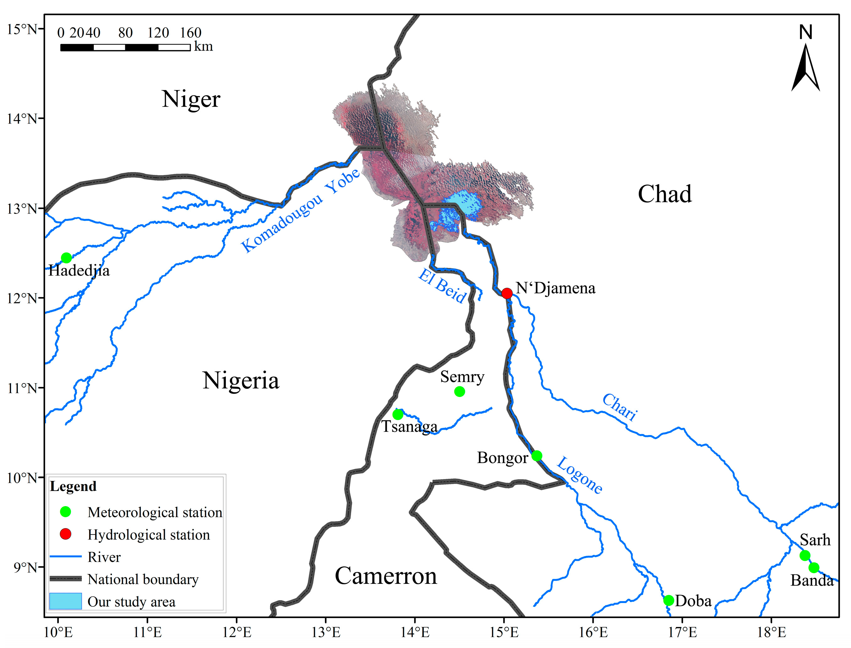
Figure 2.
The serious lake recession of Lake Chad observed from Landsat images.
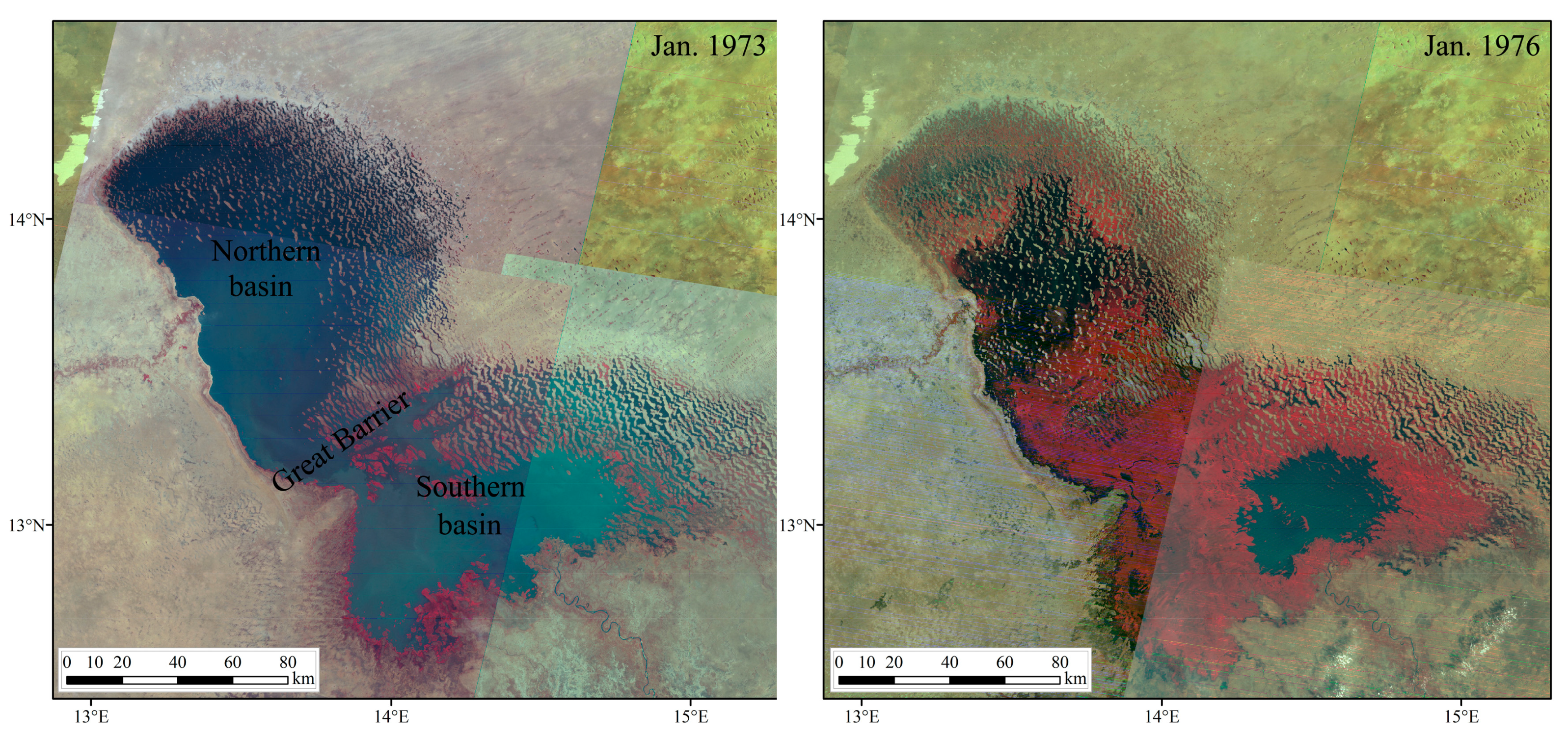
Figure 3.
Time series of monthly discharge of the Chari/Logone River, the direct rainfall of the southern pool of Lake Chad (SPLC) and the regional average rainfall of the whole basin.
Figure 3.
Time series of monthly discharge of the Chari/Logone River, the direct rainfall of the southern pool of Lake Chad (SPLC) and the regional average rainfall of the whole basin.

Figure 4.
Seasonal variations of river discharge and regional average rainfall of the whole basin.

Figure 5.
Water level variations retrieved from four altimetry products: GRLM (a), Hydroweb (b), DAHITI (c), RLH (d). The red lines indicate the trend of variation.
Figure 5.
Water level variations retrieved from four altimetry products: GRLM (a), Hydroweb (b), DAHITI (c), RLH (d). The red lines indicate the trend of variation.

Figure 6.
Scatterplots of the water surface area extracted from Landsat images and water level retrieved from: Hydroweb (a); GRLM (b); and DAHITI (c) products. The black, red and green colors in GRLM product represent OSTM, Jason-1 and T/P dataset, respectively.
Figure 6.
Scatterplots of the water surface area extracted from Landsat images and water level retrieved from: Hydroweb (a); GRLM (b); and DAHITI (c) products. The black, red and green colors in GRLM product represent OSTM, Jason-1 and T/P dataset, respectively.
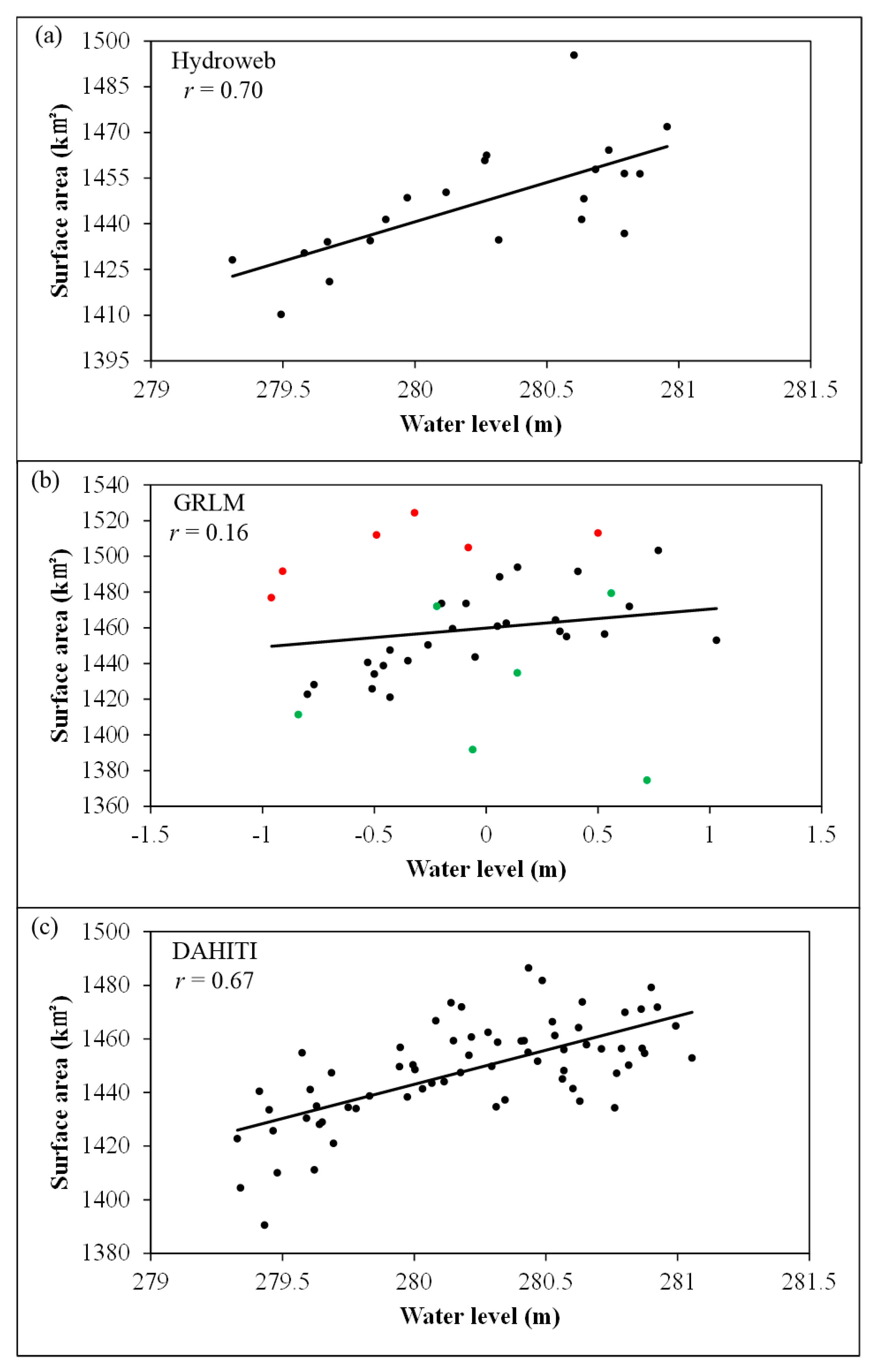
Figure 7.
Scatterplots of the water levels retrieved from: Hydroweb (a); and GRLM/OSTM (b), and the corresponding water levels retrieved from DAHITI.
Figure 7.
Scatterplots of the water levels retrieved from: Hydroweb (a); and GRLM/OSTM (b), and the corresponding water levels retrieved from DAHITI.
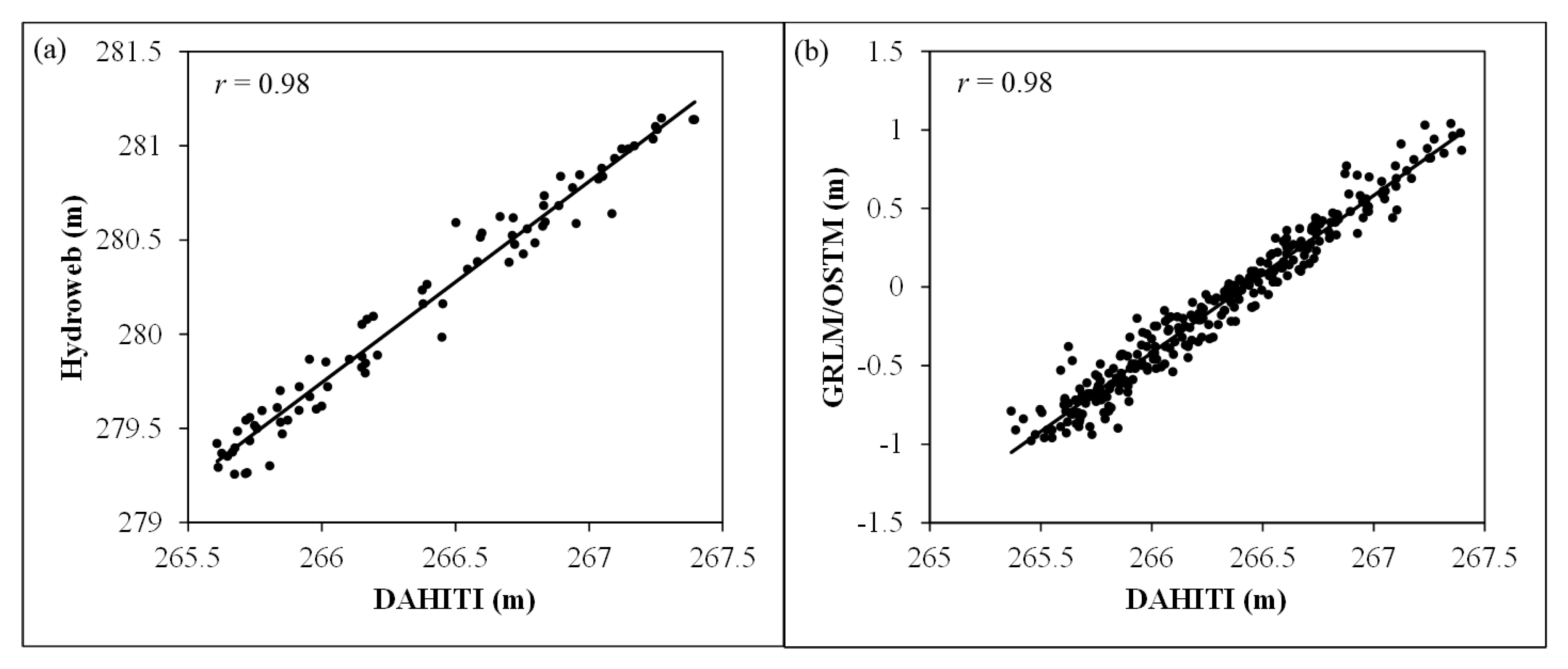
Figure 8.
Time series of water level on days when the observations of all three altimetry products are available.
Figure 8.
Time series of water level on days when the observations of all three altimetry products are available.

Figure 9.
Variations of water levels retrieved from the combination of Hydroweb, GRLM/OSTM and DAHITI.
Figure 9.
Variations of water levels retrieved from the combination of Hydroweb, GRLM/OSTM and DAHITI.

Figure 10.
Monthly average water level of the SPLC from 1992 to 2016.

Figure 11.
Time series of water levels observed in June and November.

Figure 12.
The water level-surface area (L-A) curve retrieved for the SPLC (a); and its accuracy for lake surface area estimates (b).
Figure 12.
The water level-surface area (L-A) curve retrieved for the SPLC (a); and its accuracy for lake surface area estimates (b).

Figure 13.
Variations of lake surface area of the SPLC retrieved from the L-A curve.

Figure 14.
Monthly average lake surface area of the SPLC from 1992 to 2016.

Figure 15.
Time series of lake surface area retrieved in June and November.
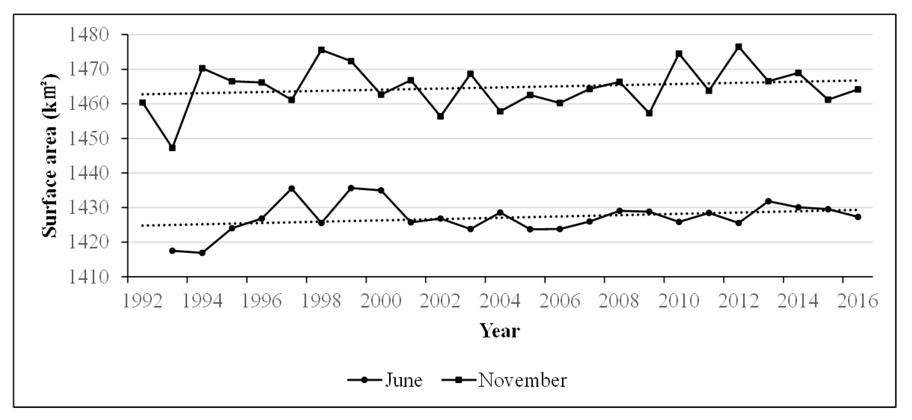
Figure 16.
Variation of of the SPLC on: daily (a); and monthly (b) scale.

Figure 17.
Monthly average water volume variation of the SPLC from 1992 to 2016.

Figure 18.
Correlations between and precipitation of: the same month (a); the prior month (b); the second month prior to the same (c); and the third month prior to the same (d).
Figure 18.
Correlations between and precipitation of: the same month (a); the prior month (b); the second month prior to the same (c); and the third month prior to the same (d).

Figure 19.
Scatterplots of retrieved from remote sensing observations and retrieved from the regression model.
Figure 19.
Scatterplots of retrieved from remote sensing observations and retrieved from the regression model.

Figure 20.
Time series of the Water Volume Above the Lowest water Level (WVALL) retrieved from the L-V curve.
Figure 20.
Time series of the Water Volume Above the Lowest water Level (WVALL) retrieved from the L-V curve.
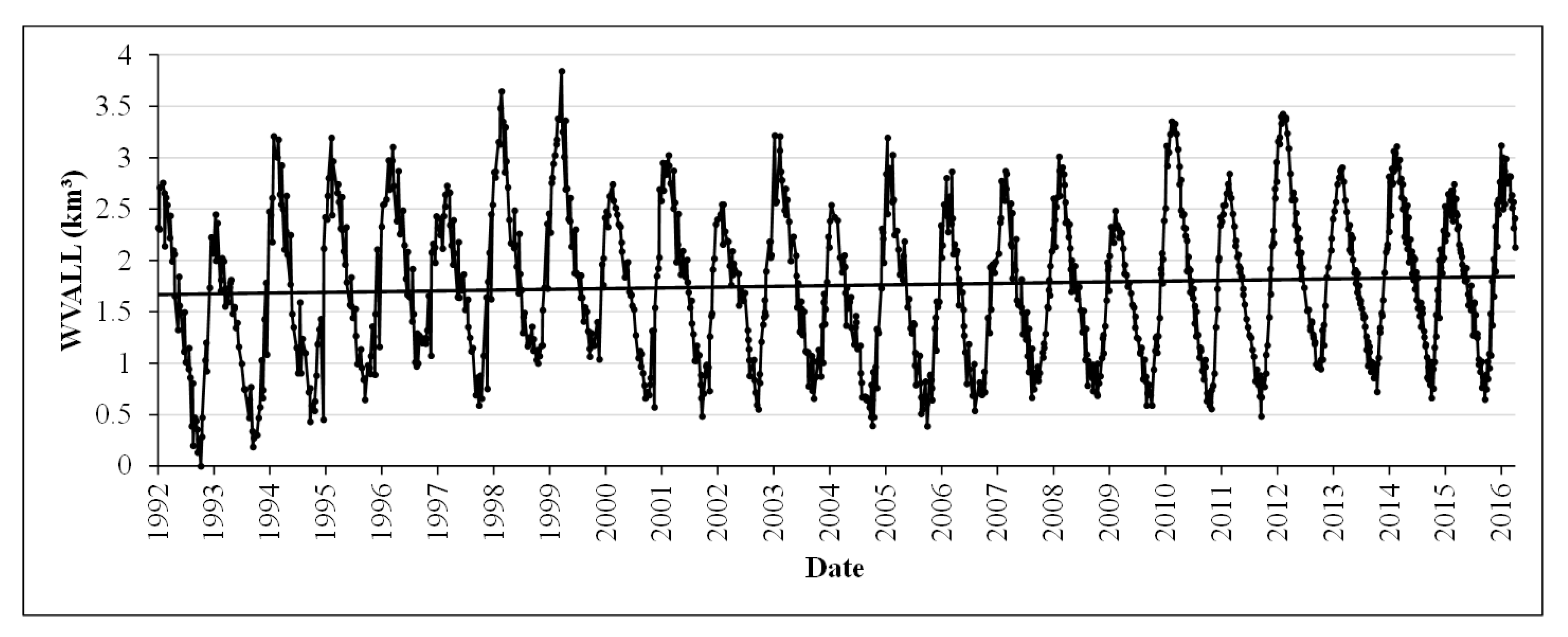
Figure 21.
Monthly average WVALL of the SPLC from 1992 to 2016.

Figure 22.
Variations of different water budget components of the SPLC from 1992 to 2016.

Figure 23.
Scatterplots of precipitation and evaporation observations versus those retrieved from CRU product.
Figure 23.
Scatterplots of precipitation and evaporation observations versus those retrieved from CRU product.


Table 1.
Monthly mean values (km3) for the components of the SPLC water budget.
| Month | |||||
|---|---|---|---|---|---|
| 1 | −0.37 | 1.03 | 0.00 | 0.31 | 1.09 |
| 2 | −0.30 | 0.54 | 0.00 | 0.33 | 0.51 |
| 3 | −0.29 | 0.38 | 0.00 | 0.41 | 0.26 |
| 4 | −0.31 | 0.24 | 0.00 | 0.41 | 0.15 |
| 5 | −0.29 | 0.28 | 0.02 | 0.40 | 0.19 |
| 6 | −0.18 | 0.49 | 0.08 | 0.35 | 0.40 |
| 7 | 0.11 | 1.40 | 0.17 | 0.30 | 1.15 |
| 8 | 0.47 | 2.88 | 0.24 | 0.26 | 2.39 |
| 9 | 0.68 | 4.38 | 0.14 | 0.29 | 3.55 |
| 10 | 0.55 | 5.89 | 0.02 | 0.33 | 5.04 |
| 11 | 0.19 | 4.32 | 0.00 | 0.33 | 3.80 |
| 12 | −0.24 | 2.09 | 0.00 | 0.31 | 2.01 |
| Total | 0.01 | 23.91 | 0.67 | 4.03 | 20.54 |
Table 2.
Comparison of water budget components (km3) estimated in different studies.
| Study | Time Period | Study Area | ||||
|---|---|---|---|---|---|---|
| LCBC [30] | 1954–1969 | Lake Chad | 7.4 | 48.8 | 44.2 | 2.5 |
| Odada et al. [3] | Pre-1970 | Lake Chad | 6.0 | 43 | 42.89 | 3 |
| Odada et al. [3] | 1971–1990 | Lake Chad | 2.1 | 23.1 | 22.57 | 1.4 |
| LCBC [30] | 1988–2010 | Lake Chad | 1.9 | 22.6 | 21.9 | 1 |
| This study | 1991–2013 | SPLC | 0.67 | 4.03 | 23.91 | 20.54 |
© 2017 by the authors. Licensee MDPI, Basel, Switzerland. This article is an open access article distributed under the terms and conditions of the Creative Commons Attribution (CC BY) license (http://creativecommons.org/licenses/by/4.0/).
Share and Cite
MDPI and ACS Style
Zhu, W.; Yan, J.; Jia, S. Monitoring Recent Fluctuations of the Southern Pool of Lake Chad Using Multiple Remote Sensing Data: Implications for Water Balance Analysis. Remote Sens. 2017, 9, 1032. https://doi.org/10.3390/rs9101032
AMA Style
Zhu W, Yan J, Jia S. Monitoring Recent Fluctuations of the Southern Pool of Lake Chad Using Multiple Remote Sensing Data: Implications for Water Balance Analysis. Remote Sensing. 2017; 9(10):1032. https://doi.org/10.3390/rs9101032
Chicago/Turabian StyleZhu, Wenbin, Jiabao Yan, and Shaofeng Jia. 2017. "Monitoring Recent Fluctuations of the Southern Pool of Lake Chad Using Multiple Remote Sensing Data: Implications for Water Balance Analysis" Remote Sensing 9, no. 10: 1032. https://doi.org/10.3390/rs9101032
Note that from the first issue of 2016, this journal uses article numbers instead of page numbers. See further details here.