Improving Classification Accuracy of Multi-Temporal Landsat Images by Assessing the Use of Different Algorithms, Textural and Ancillary Information for a Mediterranean Semiarid Area from 2000 to 2015

Abstract

The aim of this study was to evaluate three different strategies to improve classification accuracy in a highly fragmented semiarid area using, (i) different classification algorithms with parameter optimization in some cases; (ii) different feature sets including spectral, textural and terrain features; and (iii) different seasonal combinations of images. A three-way ANOVA was used to discern which of these approaches and their interactions significantly increases accuracy. Tukey–Kramer contrast using a heteroscedasticity-consistent estimation of the kappa covariances matrix was used to check for significant differences in accuracy. The experiment was carried out with Landsat TM, ETM and OLI images corresponding to the period 2000–2015. A combination of four images using random forest and the three feature sets was the best way to improve accuracy. Maximum likelihood, random forest and support vector machines do not significantly increase accuracy when textural information was added, but do so when terrain features were taken into account. On the other hand, sequential maximum a posteriori increased accuracy when textural features were used, but reduced accuracy substantially when terrain features were included. Random forest using the three feature subsets and sequential maximum a posteriori with spectral and textural features had the largest kappa values, around 0.9.

1. Introduction

Several factors hinder the classification of remote sensing imagery in Mediterranean landscapes: the high heterogeneity, due to the presence of small patches dedicated to several different land uses and covers [1]; urban sprawl [2]; the high reflectivity of very dry soils and limestone areas that mask the presence of vegetation [3]; and finally, when rainfed and irrigated areas are mixed, they may be difficult to distinguish by using a single scene image for the analysis [4].

Several strategies have been developed to overcome these difficulties. Traditional parametric methods, such as Maximum Likelihood (ML) [5], have been substituted by more robust techniques such as Random Forest (RF) [6] or Support Vector Machine (SVM) [7]. Another interesting method, although far less used, is Sequential Maximum A Posteriori (SMAP), a Bayesian multi-scale classification algorithm [2,8,9]. Several studies have used these methods and reported the comparisons made among them. Li et al. [10] used RF, SVM and decision trees to classify forest communities in New York State (USA), obtaining better accuracy with the first two. These authors thought that machine learning non-parametric methods are more versatile than traditional ones for processing large and complicated datasets. Sluiter and Pebesma [11] compared seven classification techniques in Mediterranean heterogeneous landscapes, concluding that the most accurate results were obtained both with RF and SVM. They found that these two algorithms improved accuracy, especially when the number of classes was increased to 15, that is as the complexity of the classification increased. They also stressed how RF and SVM are able to handle large datasets with highly correlated features better than more traditional classifiers. Similar results were reported by He et al. [12] when mapping Arctic lithology in Canada. Rodríguez-Galiano [13] and Rodriguez-Galiano et al. [14] used several different methods to classify land use in a semiarid environment in southern Spain. They reached the same conclusions as the previous authors, stressing that SVM and RF are more robust in the presence of noise in the data. Belgiu and Drăguţ [15], in a recent review of previous research, concluded that the RF classifier outperforms decision trees, the Binary Hierarchical Classifier (BHC), Linear Discriminant Analysis (LDA) and artificial neural network classifiers in terms of classification accuracy; RF and SVM classifiers are equally reliable, the accuracy of RF being slightly higher for high dimensional input data such as hyperspectral imagery; however, the SVM classification is more sensitive to the selected features, and it is more complicated to use as several parameters have to be set. These authors highlight the lower sensitivity of RF, compared with other algorithms, to erroneous training data or overfitting and point to the robustness due to the ensemble of classifiers and the randomness in the selection of a feature subset when the nodes of the trees are split. McCauley and Engel [8], Ehsani [9] and Ehsani and Quiel [16] compared SMAP with ML, finding that the most accurate results were obtained with SMAP. The last author argues that this algorithm can take into account the texture and spatial information provided by the image even when they are not explicitly provided as features. Kumar et al. [17] compared SMAP with five machine learning algorithms, including RF and SVM, to classify Landsat imagery, the results obtained with SMAP being more accurate than with the machine learning algorithms. The reason for this, according to the authors, is that SMAP reaches higher accuracy values because it can retrieve information from both intra-class and spatial variability.

Other lines of research have centered on the use of ancillary data (mostly terrain features) to improve accuracy [18]. The conclusion of these studies is that spectral information is not sufficient for an accurate classification and that terrain information significantly improves accuracy, especially in vegetation types most affected by relief. After an analysis of several studies, Lu and Weng [19] stressed that terrain features improve accuracy in vegetation classification, especially in mountainous regions where vegetation distribution is closely related to topography; however, in urban studies, these features are not commonly used. Sluiter and Pebesma [11] obtained more accurate classifications using ancillary information (elevation, slope, aspect, water stress index and rock types) to complement reflectivity, especially when using RF or SVM, possibly due to the effect of soil variables, geology and soil moisture on vegetation classes. Furthermore, Kumar et al. [17] included Digital Elevation Model derived features when comparing classification methods. Other successful approaches to increase classification accuracy include the use of textural features [3,20] and the use of different images corresponding to different seasons in the same year [14,19]. Zhou and Robson [20] pointed out that texture introduces relevant information when classifying certain types of land cover in the Mediterranean region. They specifically mention the improvement in accuracy for urban classes because the objects in an urban area are so small that they form part of the distinctive texture (high frequency spatial variation) within urban areas. The use of multi-temporal information has proven useful for improving the classification accuracy in agricultural crops and other vegetation types due to changes in plant phenology. In addition, the use of multi-temporal information has been found useful when trying to separate cultivated from natural cover. Classifying multi-seasonal spectral bands using machine learning algorithms such as RF to produce land cover maps helps overcome the difficulty of discriminating between classes that have close spectral characteristics or exhibit a similar phenology [21]. Finally, Gómez et al. [22] identified and reviewed methods to incorporate time series information and other novel inputs for annual land cover characterization.

From the literature consulted, it appears that the use of auxiliary features can produce an increase in accuracy only if the algorithm is not sensitive to the Hughes effect; in this case, the potential increase in accuracy would be reduced by the decrease in sampling density, unless the number of training elements is increased exponentially (something that is not usually possible in land cover classification).

Since a suitable statistical analysis is needed to test the significance of any improvement in accuracy due to the different strategies tested and also any interaction between them, the objective of this study was to integrate the four above-mentioned approaches (machine learning algorithms, textural features, contextual features and multi-seasonal) to test their ability to increase accuracy when classifying land cover in a diversified Mediterranean semiarid area. More specifically, we try to increase classification accuracy by using: (1) machine learning algorithms with and without parameter optimization; (2) several images taken in different seasons of the same year; and (3) different feature sets including textural and contextual (terrain) information. A factorial ANOVA is used to discern which of these approaches, and their interactions, are most relevant for increasing accuracy and whether the interaction of two such approaches might have a higher impact on accuracy than the sum of individual impacts. Tukey–Kramer contrast using a heteroscedasticity-consistent estimation of the kappa covariances matrix was used to check for significant differences in accuracy when using strategies to improve accuracy.

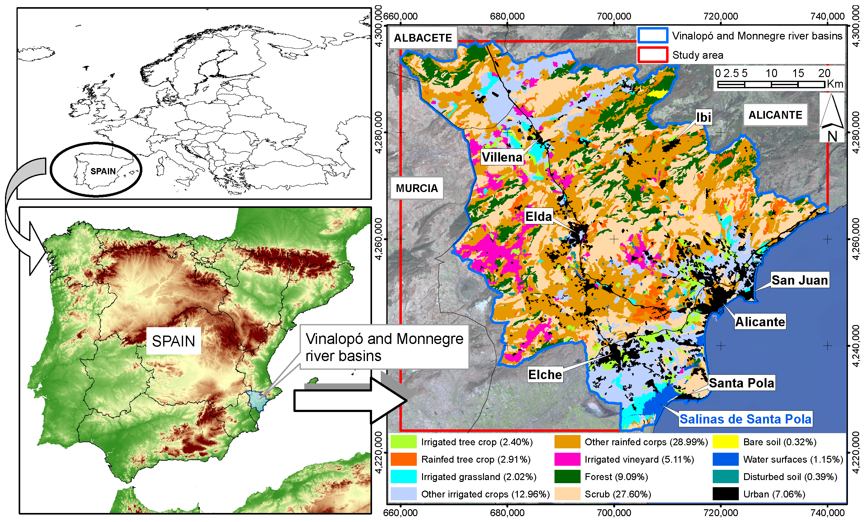
2. Study Area

The research was conducted in a 5079 km${}^2$ semiarid area in south-eastern Spain (Figure 1) in which the Vinalopó and Monnegre river basins (3003 km${}^2$) are included. Precipitation is scarce and irregular; in addition, high temperatures and many hours of sun result in high potential evapotranspiration. Human pressure is quite high, and the equivalent population (including both permanent and seasonal) is 1,087,536 [23], including large cities such as Alicante (332,067 inhabitants) and Elche (228,647 inhabitants). More than 60% of the area is dedicated to agricultural activities, mainly irrigated using groundwater and water transfers from the river Tagus. The aridity, pluviometric variability, human pressure and the irrigated agriculture combine to produce a highly diverse area. Such diversity complicates any attempt to classify remote sensing imagery.

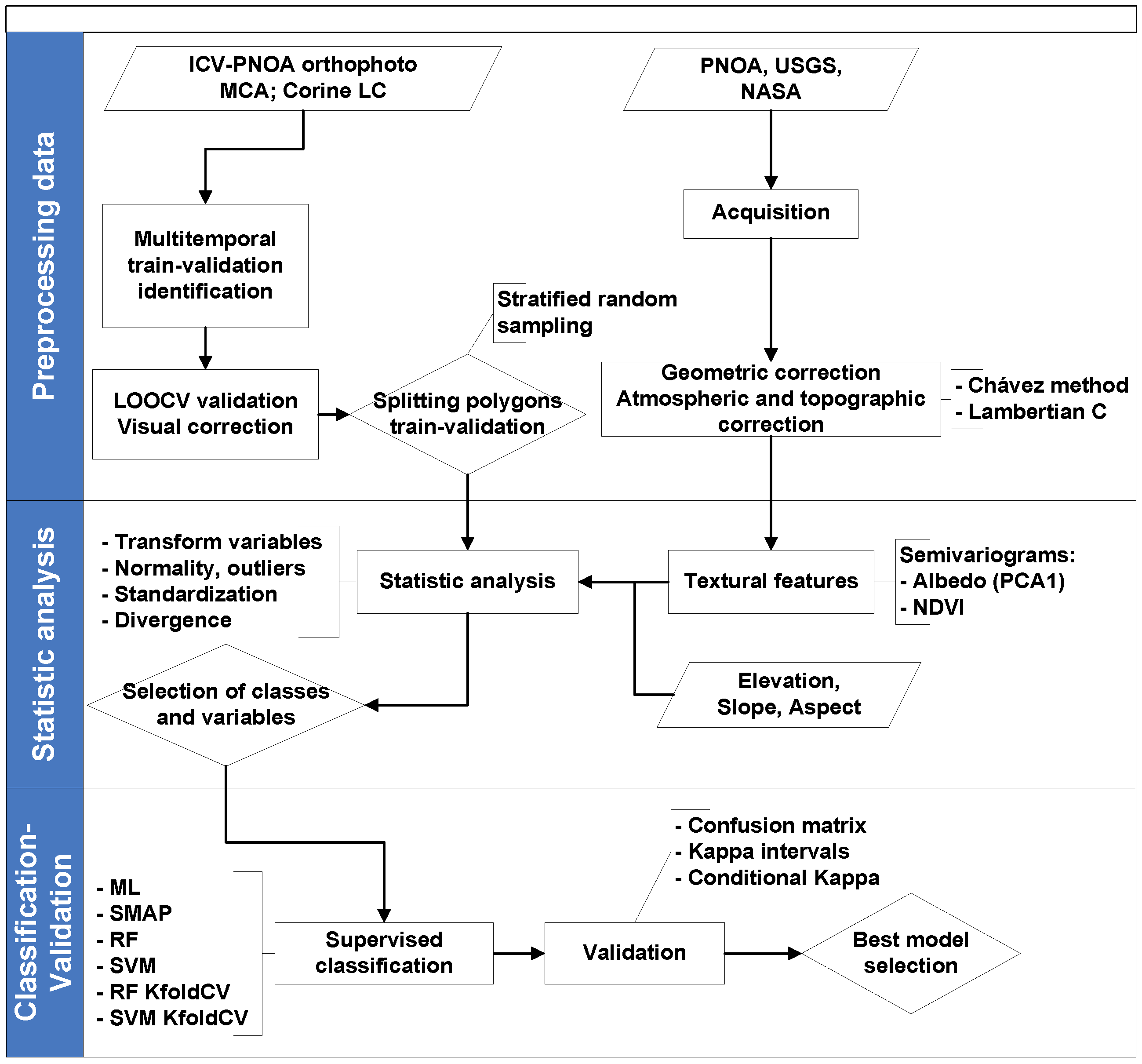
3. Material and Methods

Figure 2 shows the working process schematically. This process can be divided into three main blocks: (1) Information pre-processing, which includes the acquisition, processing and corrections of the images, and the identification and processing of training and validation sites; (2) statistical analysis of auxiliary variables, including the creation of new textural variables, and the standardization and transformation of spectral features; this section assesses the assumptions of the classification methods, such as normality, and characterizes the classes and polygons (spectral signatures, divergence, etc.); (3) classification and validation of results (process implemented in the Supplementary Material).

3.1. Data Sources

The study area is fully located in the Landsat scene with Path 199 and Row 33, occupying 18.5% of the scene. Landsat-5 Thematic Mapper (TM), Landsat-7 Enhanced Thematic Mapper Plus (ETM+) and Landsat-8 Operational Land Imager (OLI) images for the period 2000–2015, except 2012 (as we did not find images of sufficient quality to perform the experiment), were classified. When possible, four different images per year (one per season) were taken into account.

Table 1. Landsat images analyzed in this study. In bold are those used for the classification.

Date	Sensor	Date	Sensor	Date	Sensor	Date	Sensor	Date	Sensor
2000		2001		2002		2003		2004
29-Jan-00	ETM+	1-Dec-01	TM	6-Feb-03	ETM+	6-Feb-03	ETM+	4-Mar-04	TM
21-Jun-00	ETM+	21-Apr-01	ETM+	24-Apr-02	ETM+	10-March-03	TM	13-Apr-04	ETM+
8-Aug-00	ETM+	26-Jul-01	ETM+	19-Jun-02	TM	29-May-03	TM	19-Aug-04	ETM+
27-Oct-00	ETM+	30-Oct-01	ETM+	-	-	26-Sep-03	TM	15-Nov-04	TM
2005		2006		2007		2008		2009
4-Mar-04	TM	24-Jan-07	TM	24-Jan-07	TM	14-Feb-09	TM	14-Feb-09	TM
18-May-05	ETM+	6-Jun-06	ETM+	8-May-07	ETM+	19-Jun-08	TM	5-May-09	TM
26-Jun-05	TM	16-Jul-06	TM	4-Aug-07	TM	15-Sep-08	ETM+	24-Jul-09	TM
12-Dec-05	ETM+	13-Nov-06	ETM+	16-Nov-07	ETM+	1-Oct-08	ETM	10-Sep-09	TM
2010		2011		2013		2014		2015
16-Nov-10	TM	4-Feb-11	TM	-	-	16-Mar-14	OLI	2-Feb-15	OLI
24-May-10	TM	9-Apr-11	TM	14-Apr-13	OLI	4-Jun-14	OLI	7-Jun-15	OLI
11-Jul-10	TM	28-Jun-11	TM	19-Jul-13	OLI	22-Jul-14	OLI	9-Jul-15	OLI
29-Sep-10	TM	-	-	14-Nov-13	OLI	26-Oct-14	OLI	30-Nov-15	OLI

shows the 54 images analyzed. After a preliminary quality and cloudiness analysis, 42 images (in bold in Table 1) were finally used. In some years, it was not possible to find good winter images, so the corresponding image from the previous or subsequent year was used.

To have a coherent georeferentiation for TM and ETM images, we used 35 control points homogeneously distributed throughout the study area and identifiable in all the images; RSME values were, in all cases, lower than the pixel size. Landsat-8 images are delivered with sufficiently accurate georeferentiation. Atmospheric correction was carried out using the method of Chávez [25] and topographic correction using [26].

3.2. Classification Methods

To test the effect of different classification methods, we used four classification algorithms, representing different approaches in remote sensing imagery classification: ML, a classical parametric method; RF, an ensemble of decision trees; SVM, a kernel-based algorithm; and SMAP, a multi-scale Bayesian method.

3.2.1. Maximum Likelihood

Assuming that features follow a normal multivariate probability distribution, the vectors of means and the variance-covariance matrices of each class can be used to estimate the probability that any given pixel belongs to that class. The pixel is then classified into the most probable class. This probability can also be used as an indicator of the classification certainty, while the classification of pixels with a maximum probability below a given threshold is rejected.

As some classes have a larger presence in the study area, the proportion of each class in the training areas can be used as the prior probability, in a Bayesian approach that uses the equation:

$$P\left(H|E\right)=\frac{p\left(E|H\right)·p\left(H\right)}{p\left(E\right)}$$

(1)

where $P\left(H|E\right)$ is the conditional probability of class H given evidence E (spectral response), $p\left(E\right)$ is the total probability of E, $p\left(H\right)$ is the prior probability of H and $p\left(E|H\right)$ is the conditional probability of E given H.

Although ML has been widely used in remote sensing, the basic normality assumption is not always met, especially when including textural or ancillary information, so this assumption should be verified. Swain and Davis [27] suggest that ML may be robust enough and not affected by non-normality; however, it is very sensitive to outliers that may easily appear, especially if ancillary data are used.

3.2.2. Random Forest

RF [6] is a non-parametric method based on an ensemble of decision trees. Each tree is trained with a bootstrapped sub-sample of cases, and decisions in each node are made using just a random feature subset. Each tree contributes with one vote to classify each pixel, which, finally, is attributed to the most voted for class. The feature randomization reduces the correlation among trees, enforcing the ensemble concept. The default values of the number of trees ($ntree$) and the number of features used to train each tree ($mtry$) are, respectively, 500 trees and the square root of the number of available features rounded to the closest integer [28,29].

RF produces more accurate results than other classification methods [6,28], even when there are more features than observations or when most of the features are noisy. It is less prone than others to overfitting the model to the data [30] and gives a high generalization capability [6,31,32]. Since the cases not included in a bootstrapped sample are not used to fit the corresponding tree, they can be used to perform a cross-validation accuracy estimation [33]. However, it has been suggested [34] that this procedure may underestimate errors in remote sensing applications. A final advantage is that it is computationally lighter than other meta-classifiers such as boosting [14].

One disadvantage of RF is that, unlike other methods such as ML or logistic regression, it is difficult to obtain insights into the effects of the different features involved in the model. However, it provides a rank of feature importance that determines which features have had higher weight during the decision process [6,28,29]. It can be used to compare the relative importance among features, so the result is easier to interpret than with other algorithms such as neural networks or SVM.

3.2.3. Support Vector Machines

SVM [35,36] is a very flexible classification algorithm that draws border hyperplanes among classes in the feature space. The distance between such hyperplanes and the cases closest to them, the so-called support vectors, is maximized. These large distances, margins in SVM terminology, give SVM a greater generalization capacity, because they maximize the probability of correctly classifying new cases located between two different classes. When the classes are not completely separable, a cost parameter C penalises the number of cases allowed on the wrong side of the separating hyperplane. The higher the cost, the more complex the hyperplane to avoid misclassifications and the lower the generalization capacity. SVM uses a default value of $C=1$.

SVM is included in the category of kernel methods because kernel functions can be used to transform the feature space in order to obtain a linear separation hyperplane, even if the borders between classes in the original feature space are not linear. With the Radial Basis Function (RBF), the kernel used in this study, the $\gamma$ parameter, controls the width of the function. Generally, low $\gamma$ values produce overfitting, and very high $\gamma$ values produce underfitting.

SVM is increasingly used because of its advantages over traditional methods. Mountrakis et al. [37] analyzed several studies on SVM used in remote sensing, highlighting its good results due to its generalization ability and high reliability even with limited training data (both in quality and quantity). Nowadays, it is a fully-established method in machine learning [7,38] due to its high generalization ability compared with other algorithms such as neural networks. It was first applied to classify hyperspectral imagery by Gualtieri and Cromp [39] and Melgani and Bruzzone [40]. Recent reviews on the subject can be found in Tso and Mather [41] or Camps-Valls and Bruzzone [36].

As with RF, it is difficult to understand the effect of the different features on the model; moreover, and noisy or co-linear features can affect the results [42].

3.2.4. Sequential Maximum A Posteriori

SMAP [43,44] is based on contextual classification, a classification of the pixels by region and not individually; in this sense, it can also be considered a segmentation method. It is assumed that the cells that are close in the image are more likely to belong to the same class, so it works by dividing the image into various resolutions. It then uses coarser divisions to obtain a prior density function from which, using a Bayesian approach, an a posteriori distribution in the finer division is obtained [44,45]. The end result is a land use map with larger and more homogeneous polygons that avoid the speckle effect usual in land use maps obtained by image classification.

The only parameter to be defined is the window size, whose purpose is to divide the image to reduce the memory load; however, it can slightly influence the results as the smoothing parameters of the segmentation algorithm are estimated separately for each window. For this reason, using a small window is recommended. A similar approach is the use of Random Markov Fields (MFR) [41], although such algorithms are computationally more intensive than SMAP [44].

3.3. Multi-Seasonal Approach

To test whether the use of multi-seasonal images improves the accuracy of classification, seven season combinations were used, spring, summer, autumn, winter, winter + summer, winter + spring + summer, and the combination of the four seasons. After analyzing the 2009 images, we concluded that summer images produce the best results when used alone. As a consequence, only the summer image was used to represent one-season classifications for the rest of the years.

3.4. Feature Sets

In order to test the effect of textural and ancillary information on classification accuracy, images were classified using three different feature sets: (1) reflectivity: the six Landsat reflectivity bands; (2) reflectivity and texture estimated by two semivariogram layers; (3) reflectivity, texture and terrain features (height, slope and aspect sine and cosine) calculated from the Spanish Instituto Geográfico Nacional (National Geographic Institute) DEM, a 25-m resolution raster layer derived from LIDAR data taken in 2009. The Landsat images were resampled to align with these data using nearest neighbors to preserve the original values.

The two semivariogram layers were calculated from the first principal component of the reflectivity bands (considered as a weighted average of reflectivities) and from the NDVI, respectively. The equation used to calculate the semivariogram is:

$$\gamma =\frac{{\sum }_{i=1}^4{\left(b-b_i\right)}^2}{8}$$

(2)

where b is the value in the analyzed cell and $b_i$ the value in the four cells surrounding; so, this can be considered a one-pixel lag semivariogram.

The use of parametric classification methods such as ML requires a number of assumptions about the features: mainly that they follow a normal multivariate distribution and the absence of outliers. We analyzed these assumptions for the original and transformed variables (logarithmic and inverse) using an exploratory analysis based on box-plots and the Kolmogorov–Smirnov test. A compromise transformation for all classes was selected for each feature that did not comply with those assumptions. Finally, reflectivity and terrain features were not transformed, and textural features were logarithmically transformed.

3.5. Training and Validation Areas

One of the greatest difficulties when historical images are classified is to obtain training and validation areas for the whole period without field work. To identify such areas, we used 3 land use maps and 5 orthoimages, in order to cover the time span from 2000–2015:

• Mapa de Cultivos y Aprovechamientos (crops and land-use map) published by the Spanish Ministerio de Agricultura, Pesca y Alimentación (Ministry of Agriculture, Fisheries and Food) with field data collected between 2001 and 2007 at a 1:50,000 scale.
• Corine Land Cover maps [24] for 2000 and 2006 at a 1:200,000 scale.
• 2002 orthophotography from the Sistema de Información Geográfica de Parcelas Agrícolas (Agricultural Plots Geographic Information System) project at a 1:5000 scale by the Spanish Ministerio de Agricultura, Pesca y Alimentación (Ministry of Agriculture, Fisheries and Food).
• Orthophotography series available in the Instituto Cartográfico de Valencia (Cartographic Institute of Valencia) and the Plan Nacional de Ortofotografía Aérea (Spanish Orthophotography National Plan, PNOA) for 2005, 2007 and 2012 at a 1:10,000 scale by the Spanish Instituto Geográfico Nacional (National Geographic Institute).
• Orthophotography from the PNOA for 2009 and 2014 at a 1:5000 scale.

The criteria for selecting training and validation areas were: (1) training and validation areas should not be too close in order to guarantee statistical independence; (2) land use should be the same throughout the study period to ensure that no changes occurred; (3) to avoid border effects, areas should be defined inside the real land use polygon, discarding a 50–75-m buffer from their border; (4) infrastructures crossing the areas and other features that could introduce noise should be avoided; (5) the topography inside the areas should be as homogeneous as possible; (6) areas should be as homogeneously distributed as possible; (7) the minimum size of the training set should be between 10- and 30-times the number of features per class (at least in classifications with one or two seasons), as recommended by Mather and Koch [46]; (8) for the validation areas, the area of each land use should be proportional to its area in the Corine land cover map.

In order to address Criteria (6), (7) and (8), a previous stratified random sampling was carried out with the R SamplingStrata package (Barcaroli, 2014), using Corine’s land uses as strata. The number of points per stratum was proportional to the area of the land cover. The training (validation) area should be taken within a distance of 1000 meters from the point (Criterion (1)). Once the sampling points have been obtained, the polygons are digitized based on Criteria (2)–(5), from the photointerpretation of the orthophotos of different periods, auxiliary information on land use and false-color compositions of the scenes included in the study.

Training and validation areas obtained from maps rather than from field work are less reliable, especially when, in a multi-temporal experiment, maps are not available for every year. In order to detect pixels that in certain years might have a different use, an ML-based cross-validation analysis of each pixel and year was made to identify those pixels that, in certain years, have a very low probability of being classified in the class to which they belong according to the maps. These pixels, which were considered noisy and so eliminated, were mostly outliers, so this also functioned as an implicit outlier elimination process.

Finally, 214 areas were obtained. This set was divided into 141 (2/3) training areas and 73 (1/3) validation areas, by means of a stratified random sampling based on the classes studied and elevations in the study area (

Table 2. Number and area (ha) of training and validation areas. Water surfaces include some sea polygons. The percentages refer to the areas. Bare soil was initially included within the scrub class, but because of its different reflectivity, we have considered it as a new class.

	Training Areas			Validation Areas
Use	N	Area	%	N	Area	%
Forest	19	328.21	13.66	10	98.35	9.79
Scrub	22	302.43	12.59	12	213.50	21.26
Rainfed tree crops	13	77.89	3.24	7	51.39	5.12
Irrigated tree crops	14	148.01	6.16	8	39.78	3.96
Rainfed grassland	15	231.85	9.65	8	111.01	11.05
Irrigated grassland	10	293.20	12.20	5	103.74	10.33
Impervious surfaces	16	423.84	17.64	7	112.86	11.24
Water surfaces	11	391.12	16.28	6	207.72	20.69
Bare soil	4	7.56	0.31	2	8.02	0.80
Vineyard	17	198.62	8.27	8	57.81	5.76
Total	141	2402.73	100	73	1004.18	100

).

To evaluate the influence of stratified random sampling in the classification, several classifications were made with randomly separated training and validation areas. The resulting changes in validation were not statistically significant.

3.6. Classification Process

The objectives were tackled in three stages. First, year 2009 was classified with all possible combinations of algorithms (4), feature subsets (3) and seasonal imagery (7), making a total of 84 classifications. In the second stage, as the above results showed that multi-seasonal classifications increased the accuracy, the whole 2000–2015 series (except 2012) was classified using the highest number of seasonal images available (two, three or four) and the 3 feature sets to optimize SVM and RF models. That made 90 optimized and 90 non-optimized classifications. The objective of this stage was to optimize the parameters of the RF and SVM method to test whether such optimization significantly improves accuracy.

Although RF is not sensitive to its parameters [28,35], it can be optimized using k-fold cross-validation with repetition [47]. Kuhn and Johnson [48] suggested using $k=10$ to calibrate RF, and, following this advice, we made a 10-fold cross-validation with 5 repetitions. The range of values tested was initially $m_{try}\in \left\{2,\rho \right\}$ (where $\rho$ is the number of features), but, after some preliminary tests, we changed it to $m_{try}\in \left\{2,12\right\}$. Both SVM parameters (C and $\gamma$) were calibrated using a method similar to that described for RF: a 10-fold cross-validation with five repetitions. In this case, $\gamma$ was estimated first using the methodology of Caputo et al. [49], implemented in the R package kernlab [50]. Once $\gamma$ was set, C was optimized for values $\left\{0.25,0.5,1,2,4,8,16,32\right\}$. To optimize the parameters, we used k-fold cross-validation: the dataset is divided into k equal groups, so that in each iteration, $k-1$ groups are used to train the algorithm, and the remaining group is used to estimate model accuracy. At the end, the highest kappa value $k_{max}$ in all iterations is identified, and from all the parameter values that produced accuracies larger than $0.85\times k_{max}$, the least complex is chosen as the optimal one. The reason is that the parameters associated with the best accuracy might overfit the model [51], so it is preferred, among all the parameter values that produce reasonably high accuracies, to select the least complex model. In the case of RF, this means less trees and less features per node; in the case of SVM, a larger C means a more complex hyperplane separating the classes.

In a third stage, we classified the whole 2000–2015 period (except 2009, which was classified in the first stage, and 2012 for which there was no appropriate images). Such classifications were carried out using the 3 feature subsets, the 4 classification algorithms and 4 seasonal combinations: summer (the season with more accurate results when used alone in 2009), spring + summer, spring + summer + winter and the four-image combination. That makes 552 classifications including 2009. As the results of the second stage showed that optimization does not significantly increase accuracy, RF and SVM classifications were obtained with the default parameters.

Proprietary software was not used because of limitations to easily adapt the large number of classifications and calibration cycles, as well as the high cost. However, this work was successfully carried out using free and open source software. GRASS [52,53] was used to store raster data and to perform image preprocessing. The classification was carried out with R [54,55]. Bash and R scripting languages were used to write the computing protocols. Some advantages of such an implementation are its low cost, high interoperability between programs, easy automation of processes in high-performance servers, the modularity that allows new processes to be changed or included and the reproducibility of the work. The working server we used includes twoIntel Xeon E5620 2.4 GHz processors (16 cores), 84 Gb DDR3 1333 MHz RAM and 256 Gb SSD + 4 TB for storage. The operating system was Linux Debian.

3.7. Validation of Classifications and Evaluation of Hypothesis

To assess the quality of the results, both qualitative (visual) and quantitative (confusion matrices) analyses were carried out. Several goodness of fit statistics were estimated from the confusion matrices. The kappa index [56], introduced to remote sensing by Congalton and Mead [57], is an accuracy measurement that evaluates the percentage of improvement over a random classification [58]. The significance of differences between the indices was checked by calculating 95% confidence intervals. Kappa values were interpreted following the criteria of Landis and Koch [59], that is: 0.00–0.20, insignificant; 0.21–0.40, low; 0.41–0.60, moderate; 0.61–0.80, good; and 0.81–1.00, very good. The estimation of class accuracies involves two values: user’s accuracy, related to errors of omission, and producer’s accuracy, related to errors of commission. The goodness of fit statistics used in this study are described in detail in Congalton and Green [60].

To evaluate the effects of the different strategies to improve classification accuracy, two factorial ANOVAs considering kappa values as dependent variable were carried out:

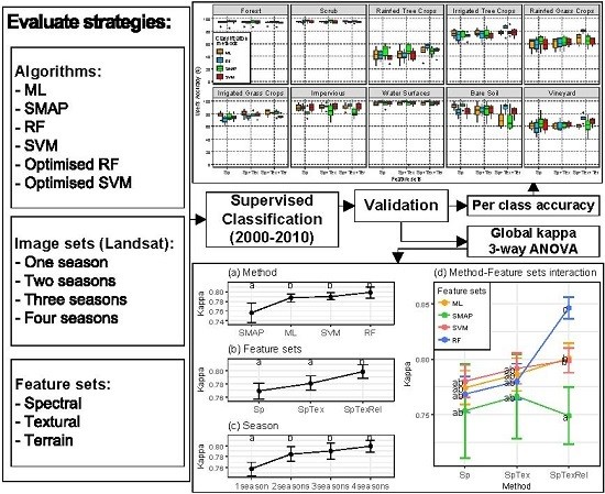
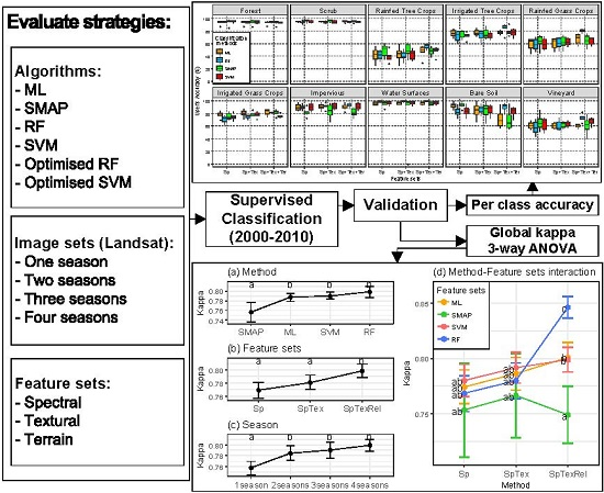
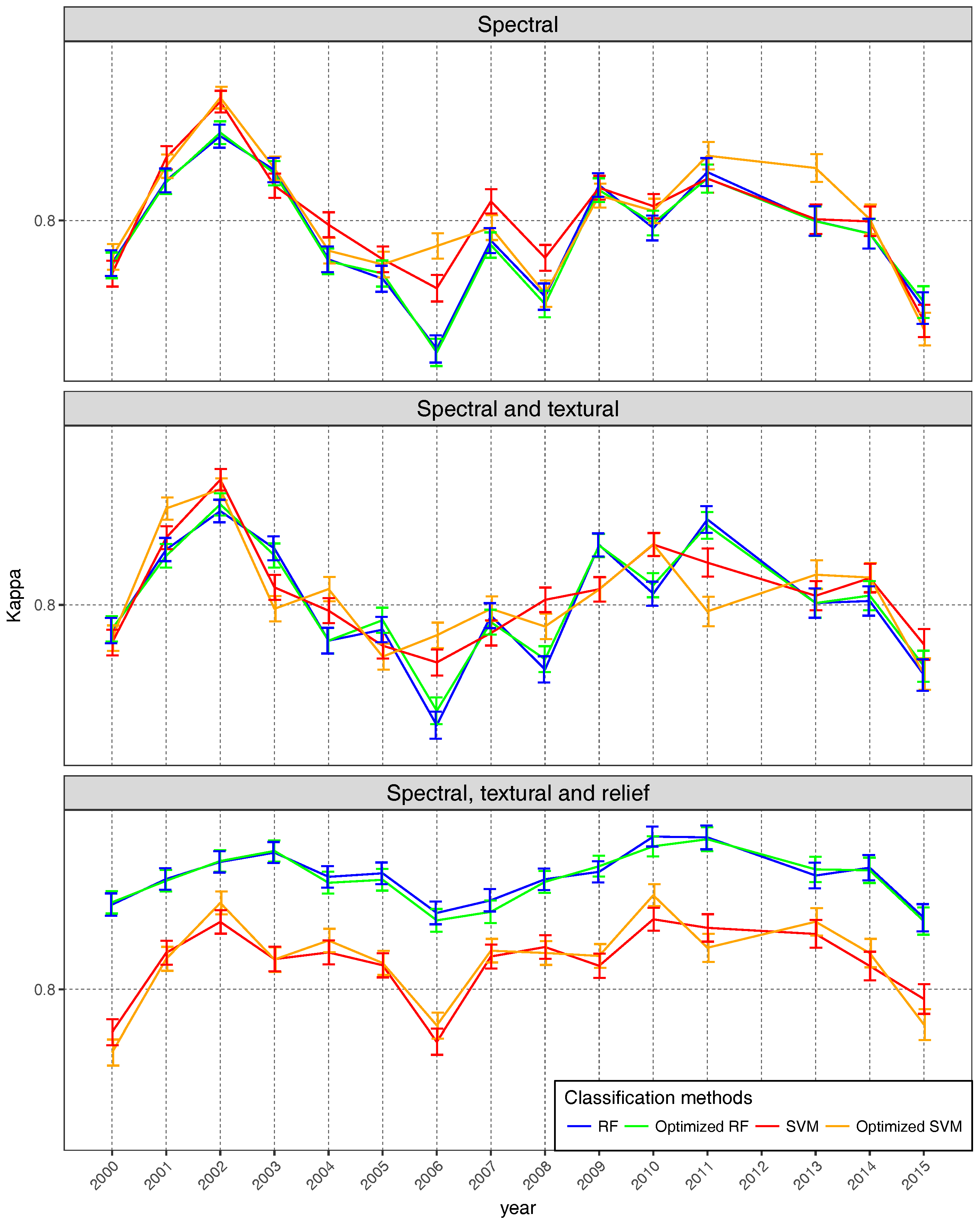
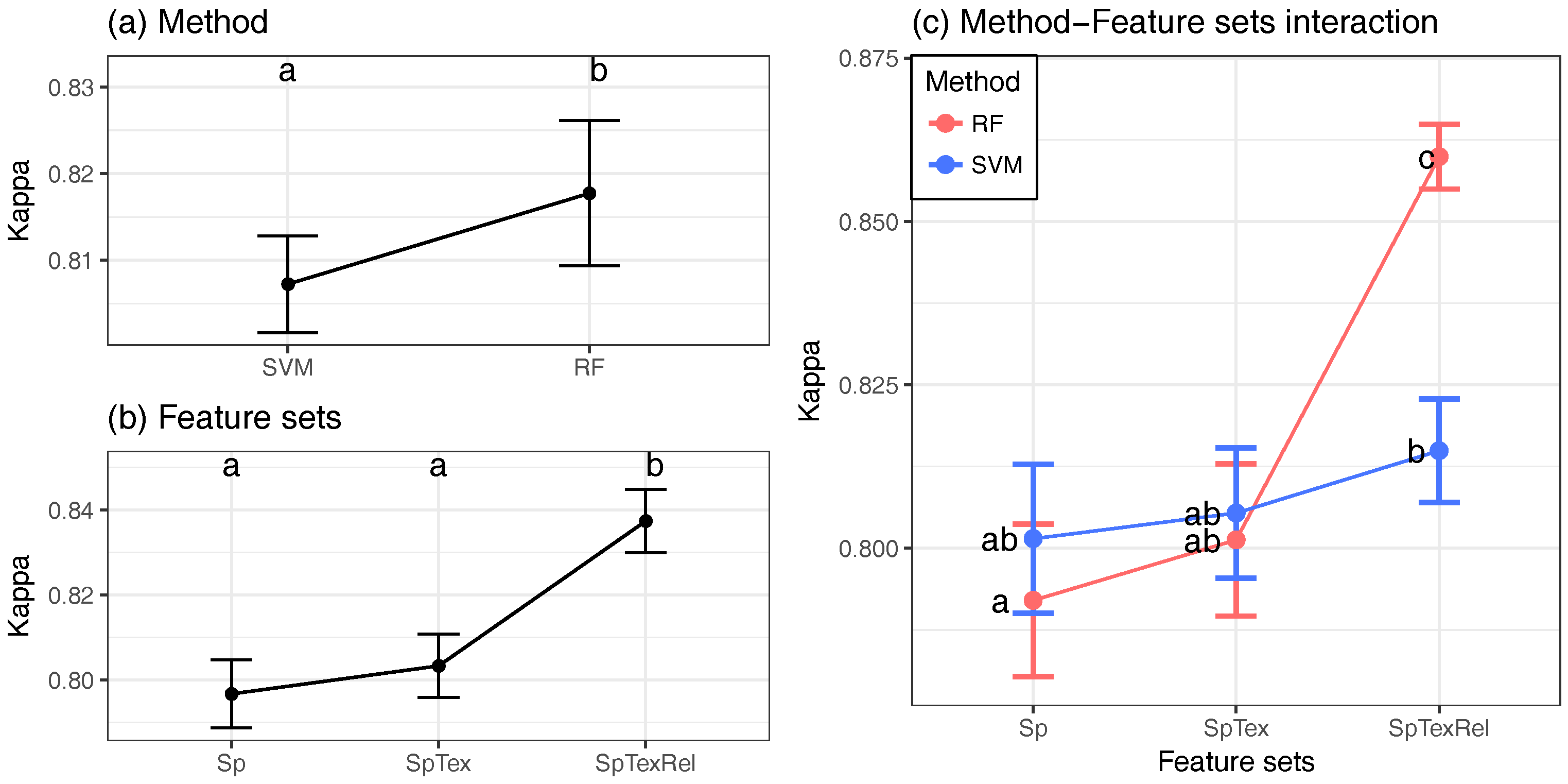
• To evaluate how the results improve when RF and SVM parameters are optimized, a factorial ANOVA was conducted to compare the effects of the classification method (method), optimization (optimized), feature sets (varset) and the interactions between them. method included two levels (RF; SVM); optimized included two levels (Yes; No); and varset three levels (Sp: Spectral information; SpTex: Spectral and Textural information; SpTexRel: Spectral, Textural and contextual information). In this case, classifications were performed using the maximum number of images available per year: four in 2000, 2001, 2009, 2010, 2014, 2015; three in 2002, 2003, 2011, 2013; and two in 2004, 2005, 2006, 2007 and 2008. That makes 180 classifications.
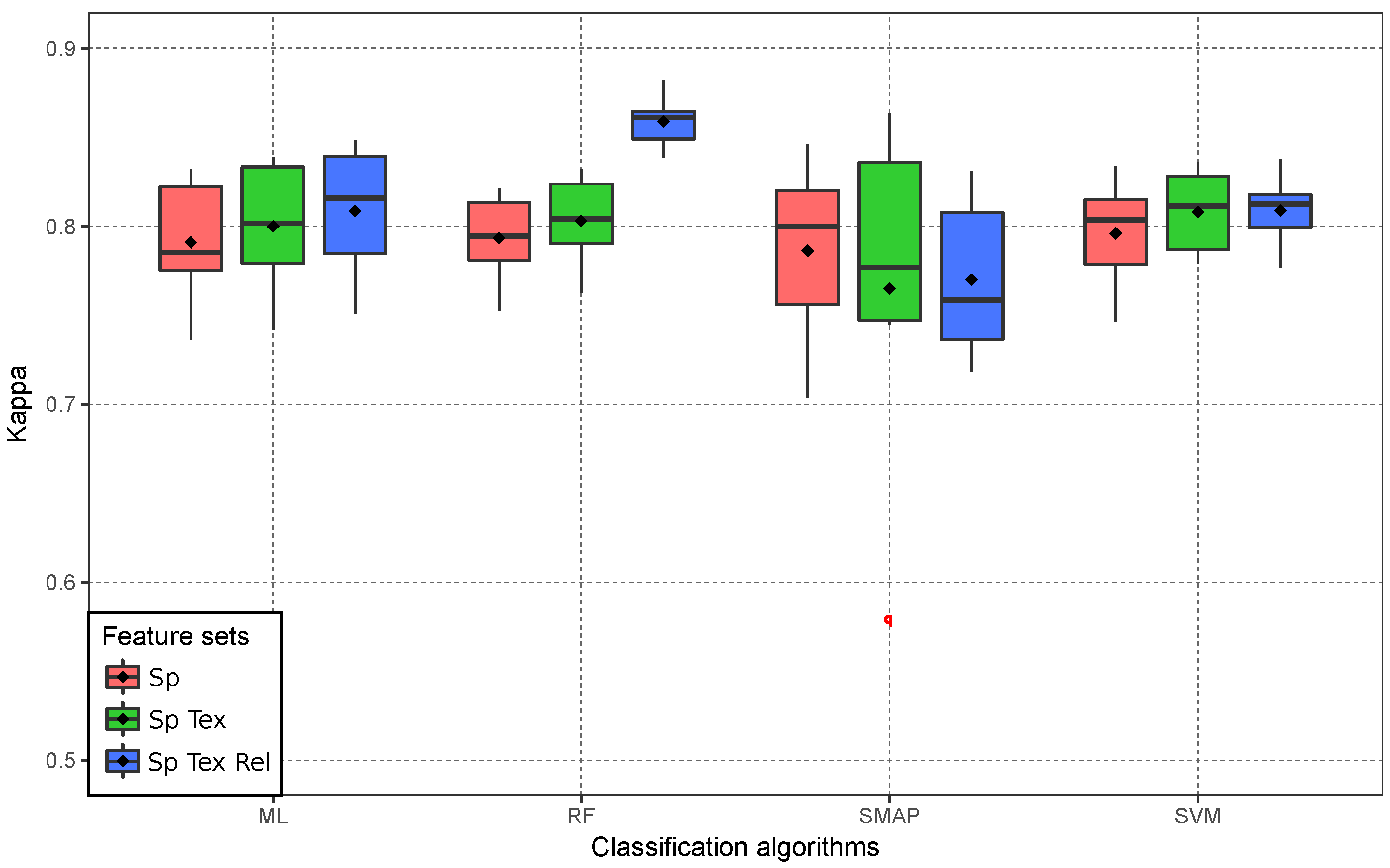
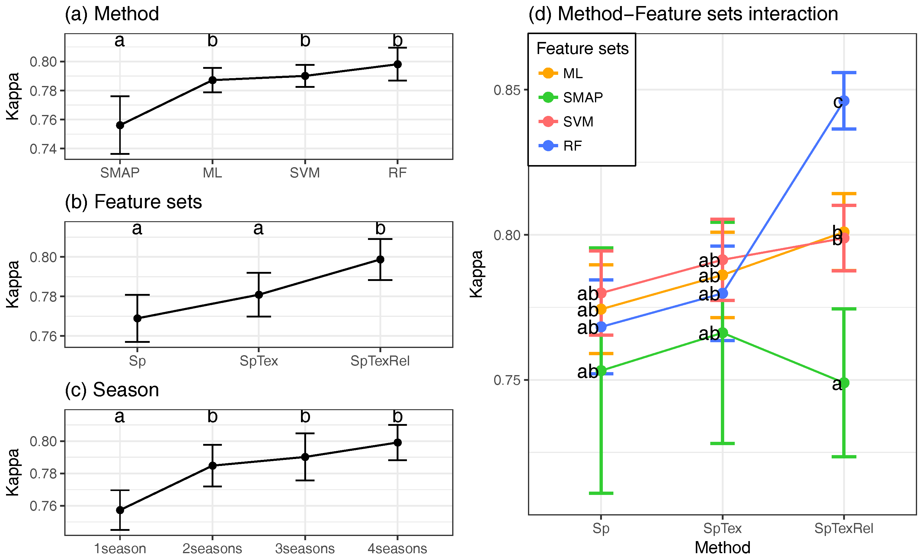
• To evaluate how classification accuracy improves in the final models, a factorial ANOVA was conducted to compare the main effects of method, varset, the number of seasonal images (season) and the interaction effect between them. In this case, method included four levels (RF; SVM; ML; SMAP) and season four levels (One season; Two seasons; Three seasons; Four seasons). In this case, only the years when 4 images were available (2000, 2001, 2009, 2010, 2014 and 2015) were taken into account, making 288 classifications.

The proposed designs include seven null hypotheses for contrast, three related to the simple effects, three related with two interactions among pairs of factors and a final one for the three factors in conjunction. The orthogonal design for three fixed levels might be represented as:

$$Y_{ijkl}=\mu +{\alpha }_j+{\beta }_k+{\gamma }_l+{\left(\alpha \beta \right)}_{jk}+{\left(\alpha \gamma \right)}_{jl}+{\left(\beta \gamma \right)}_{kl}+{\left(\alpha \beta \gamma \right)}_{jkl}+{ϵ}_{ijkl}$$

(3)

where $\mu$ is the global mean; ${\alpha }_j$, ${\beta }_k$, ${\gamma }_l$ are the effects of each level j, k y l; ${\left(\alpha \beta \right)}_{jk}$, ${\left(\alpha \gamma \right)}_{jl}$, ${\left(\beta \gamma \right)}_{kl}$ are the two-way interaction model components; ${\left(\alpha \beta \gamma \right)}_{jkl}$ are the three-way interaction model components; and ${ϵ}_{ijkl}$ is the error component.

Once the existence of an effect was discovered using ANOVA, a Tukey–Kramer contrast was carried out to identify significant differences among factors; this contrast is based on a Student’s t:

$$t=\frac{|X_i-X_j|}{S{E}_{ij}}$$

(4)

where $S{E}_{ij}$ is a pooled estimation of the standard error of the means obtained from the covariance matrix of the kappa values.

To evaluate the statistical assumptions of ML (normality and homoscedasticity), we used the Kolmogorov–Smirnov (KS) test to evaluate normality and the Levene test to evaluate homoscedasticity in the residuals. In both cases, KS was not significant ($W=0.08,p=0.2005$ and $W=0.077,p=0.066$, respectively), but the significance of the Levene contrasts ($F(11,168)=1.97,p=0.0346$ and $F(47,240)=1.95,p=0.0007$, respectively) showed heteroscedasticity. In this case, the covariance matrix of the estimated parameters ($Var[\widehat{\beta }]$) is not robust enough, and the Tukey–Kramer contrast is less reliable.

Several statistical methods have been proposed to correct for heteroscedasticity [61]. In this case, we used a heteroscedasticity-consistent covariance matrix of the parameters (HC3). With this methodology, heteroscedasticity effects are avoided even when its form is unknown [61]. The basic idea behind an HC estimator is to use residuals (${\widehat{e}}_i^2$) to estimate the covariance matrix:

$$\begin{array}{ccc}\hfill Var[\widehat{\beta }]=HC3& =& {\left(X^{\prime }X\right)}^{-1}{X}^{\prime }{\widehat{\mathsf{\Omega }}}_{3}X{\left(X^{\prime }X\right)}^{-1}\hfill \end{array}$$

(5)

$$\begin{array}{ccc}\hfill {\widehat{\mathsf{\Omega }}}_3& =& diag\left\{\frac{{\widehat{e}}_1^2}{{\left(1-h_{11}\right)}^2},\dots ,\frac{{\widehat{e}}_i^2}{{\left(1-h_{ii}\right)}^2}\right\}\hfill \end{array}$$

(6)

where $h_{ii}$ is the $ii$ element in the matrix ${\left(X^{\prime }X\right)}^{-1}{X}^{\prime }$.

Using this methodology, it is possible to compute a more robust covariance matrix estimator for the Tukey–Kramer contrast, especially when the number of cases is small.

4. Results and Discussion

4.1. Classification of 2009 Image

Figure 3 shows mean kappa and 95% confidence intervals for the four algorithms, three feature combinations and seven season combinations in 2009. With just one season, the mean kappa is M = 0.747, SD = 0.058, and with three or four seasons, the mean value is M = 0.824, SD = 0.018. High kappa values are reached; given the complexity of the study area and the objectives, the results are quite satisfactory. Figure 4 shows that using four seasons significantly outperforms any other temporal combination in every combination of algorithm and feature subset. In general, the second best option is to use three seasonal images (winter-spring-summer), which in most cases does not significantly differ from using four. When using two seasons (winter and summer), the accuracy does not significantly outperform the accuracy reached using the summer image alone, probably because it is the season in which the highest spectral differences between land uses appear. Images of winter and spring were seen to be the least accurate options.

There is a general accuracy increase when the number of features increases, especially in the case of SMAP, when spectral and textural features are introduced, and in the case of RF, when using all features.

4.2. Parameter Optimization

Having concluded that the best results are obtained with the combination of four seasons, this combination (or, when not available, the combination of three or two seasons) was used, in a second stage to classify the 2000–2015 series using RF and SVM. The objective was to test whether parameter optimization significantly improves validation accuracy. Figure 4 shows the whole 2000–2015 series of kappa values with 95% confidence intervals. An analysis of variance based on heteroscedasticity-consistent standard errors indicated that the effect optimized is not significant (F (1,168) = 0.0061, p = 0.9378), so there are no significant differences between optimized and non-optimized models (M = 0.8126, SD = 0.0346 and M = 0.8124, SD = 0.0343, respectively). By contrast, the effects of method (F (1,168) = 43.4019, p < 0.0001), varset (F (2,168) = 60.32, p < 0.0001) and the interaction between them (F (2,168) = 24.0107, p < 0.0001) were significant. Figure 5 summarizes the main and simple effects of such significant factors and the homogeneous groups obtained in the post-hoc comparisons. RF (M = 0.8177, SD = 0.04) seems significantly more accurate than SVM (M = 0.8072, SD = 0.0267); SpTexRel (M = 0.8374, SD = 0.0287, Group b) is significantly more accurate than the other two combinations (Group a); SpTex is not significantly more accurate than classifications using only spectral features, indicating that RF is significantly more accurate when using SpTexRel (M = 0.86, SD = 0.0133, Group c); in general, both methods seem to follow the same pattern, the accuracy increasing slightly when features are added to the model; however, the differences are not significant.

The main conclusion that can be drawn from these results is that optimization does not significantly improve accuracy, as the optimized model outperforms the non-optimized one only half of the time. A slightly higher accuracy is obtained with SVM when using spectral and spectral plus textural features; however, the accuracy of RF is significantly higher when adding terrain features. These results and the high computing cost of optimization, especially for RF (0.33 h without optimization and 51.2 h when optimizing), led us to omit optimization for the rest of the season combinations.

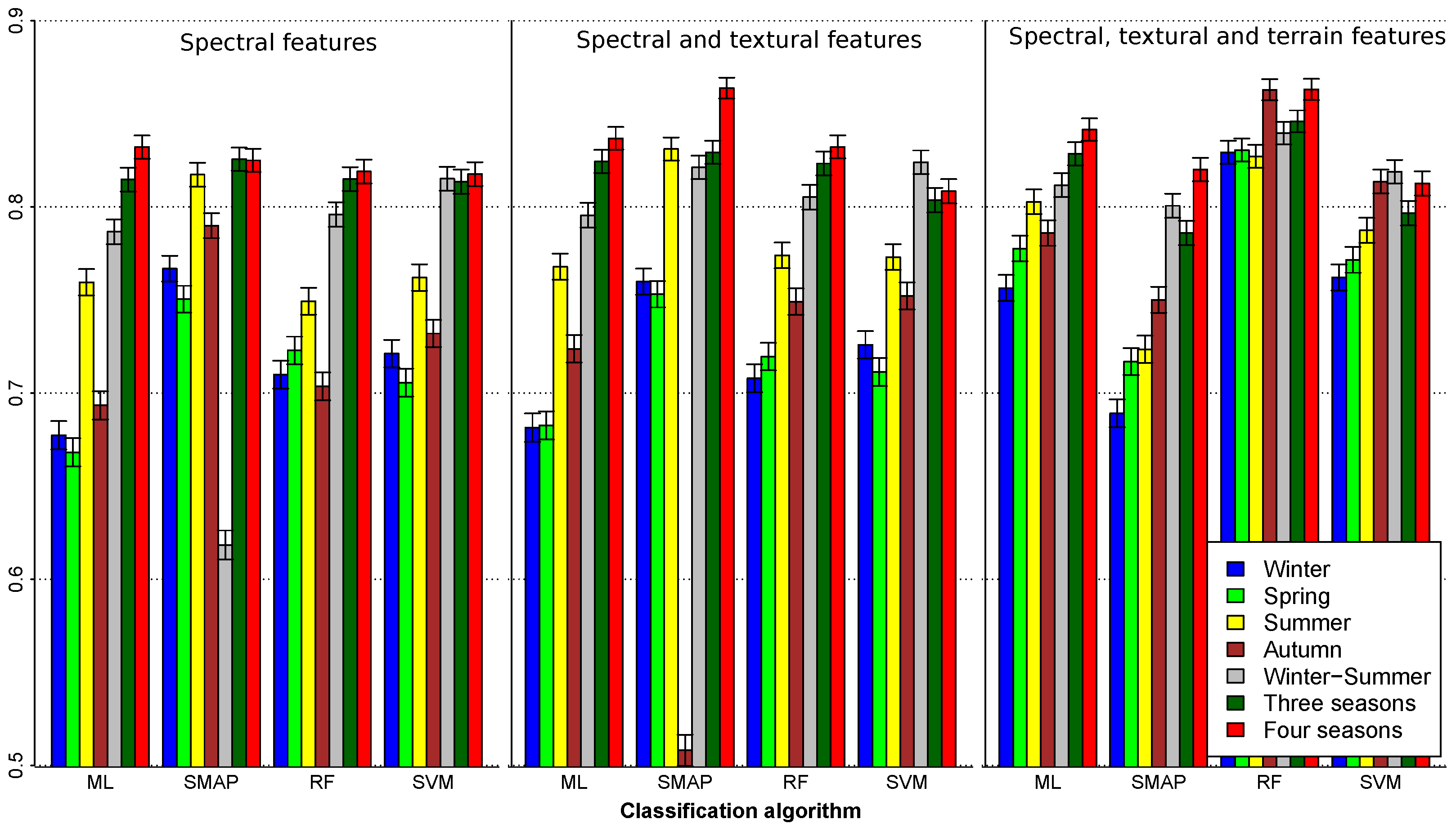
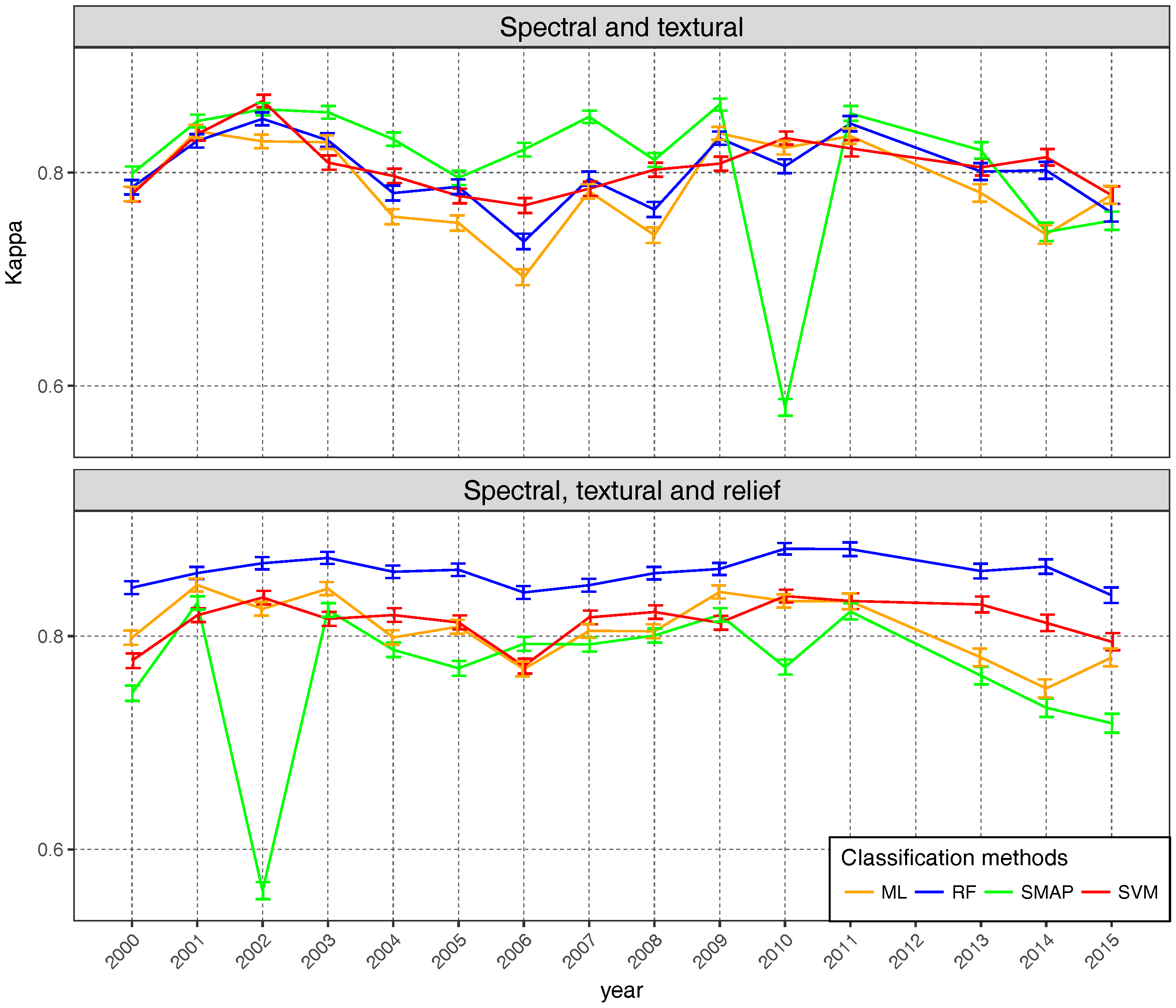
4.3. Global Validation

Figure 6 summarizes the kappa values for the period 2000–2015, and Figure 7 shows the complete series. Figure 6 does not include the period 2004–2008, because only two images per season were used in the classification for those years. According to these results, ML, RF and SVM slightly increase their accuracy when textural features are added, but the increase is higher when terrain features are taken into account, especially with RF. In contrast, SMAP improves accuracy when textural features are used, but reduces it considerably when terrain features are added, producing several moderate (lower than 0.65) kappa values. Using just two images (2004–2008) has a clear effect on classification accuracy (Figure 7). Whereas for the four-image classification (2001, 2002, 2009, 2010, 2014 and 2015), kappa values are around 0.8, which is the threshold value for a very good classification, the two-image classifications (2004–2008) drops to 0.7, except when SMAP is used to classify or when the three feature sets are taken into account.

The analysis of variance based on heteroscedasticity-consistent standard errors (conducted for the six years when four images were available) indicated that the effects on kappa values of method (F (3,240) = 14.1289, p < 0.0001), seasons (F (3,240) = 20.7537, p < 0.0001), varset (F (2,240) = 51.1315, p < 0.0001) and the interaction between method and seasons (F (6,240) = 9.6975, p < 0.0001) were significant.

As regards the main effects (Figure 8a), SMAP (M = 0.7561, SD = 0.084, Group a) is the least accurate method, whereas differences in accuracy in the other methods are not statistically significant (Group b), although RF seems slightly better. In relation to the feature sets effect (Figure 8b), the value of the SpTexRel factor (M = 0.7987, SD = 0.0512) is significantly more accurate than the others (Group b), indicating that this feature combination substantially improves accuracy. Finally, the multi-seasonal effect (Figure 8c, not evaluated when optimizing, indicates that including different images for different seasons improves accuracy since phenological differences among classes are better identified. Although the best results were obtained with four seasons (M = 0.7991, SD = 0.0467, Group b), there were no significant differences between the two-season and three-season options. Only the one-season classification (M = 0.7573; SD = 0.0523, Group a) is significantly less accurate than the others.

ML classification is usually reported to be less accurate than the machine learning methods; however, in this study, its kappa values are quite high with all feature combinations. When considering only the spectral variables, this algorithm is significantly better than RF and SVM in some years, such as 2001. In the remaining years, it provides results that are almost as good as RF and SVM. We think these results are due to the precautions taken when the training and validation areas were selected and the resulting reduction in noise and outliers in the dataset. Such results indicate that machine learning methods outperform classical statistical methods when data are noisy, indicating their greater robustness, although this is not necessarily the case when noise is removed.

Finally, although ML, RF and SVM were not significantly different, the significance of the interaction method-feature sets (Figure 8d) indicates that the accuracy of RF is significantly higher than in other methods when using the SpTexRel dataset (M = 0.8462, SD = 0.023, Group c). On the other hand, SMAP provides the lowest kappa values (M = 0.749, SD = 0.0604, Group a), while its wider confidence intervals are also of note. The four methods follow a similar pattern with a slight increase in accuracy when new features are added; however, the difference is not significant.

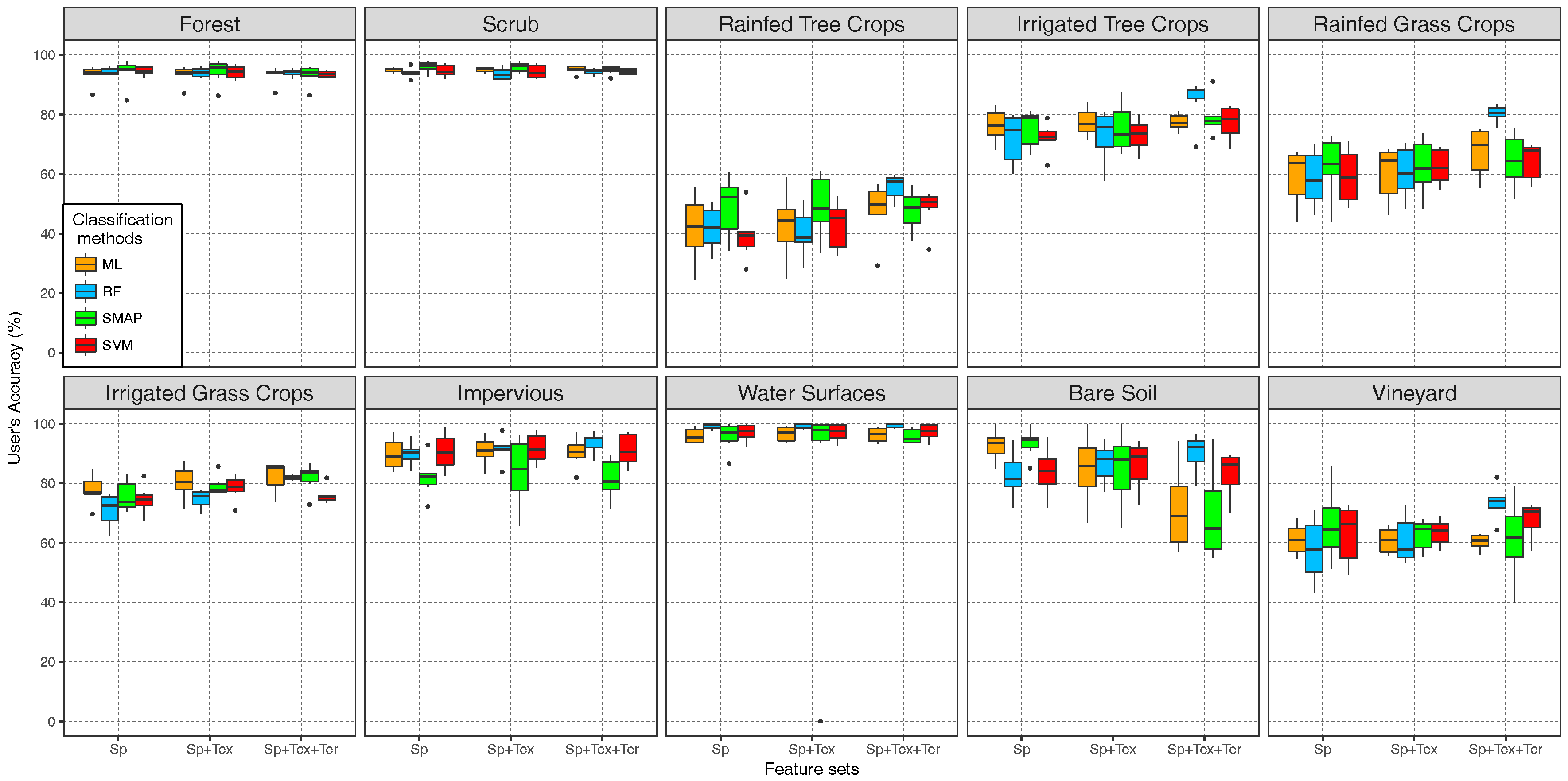
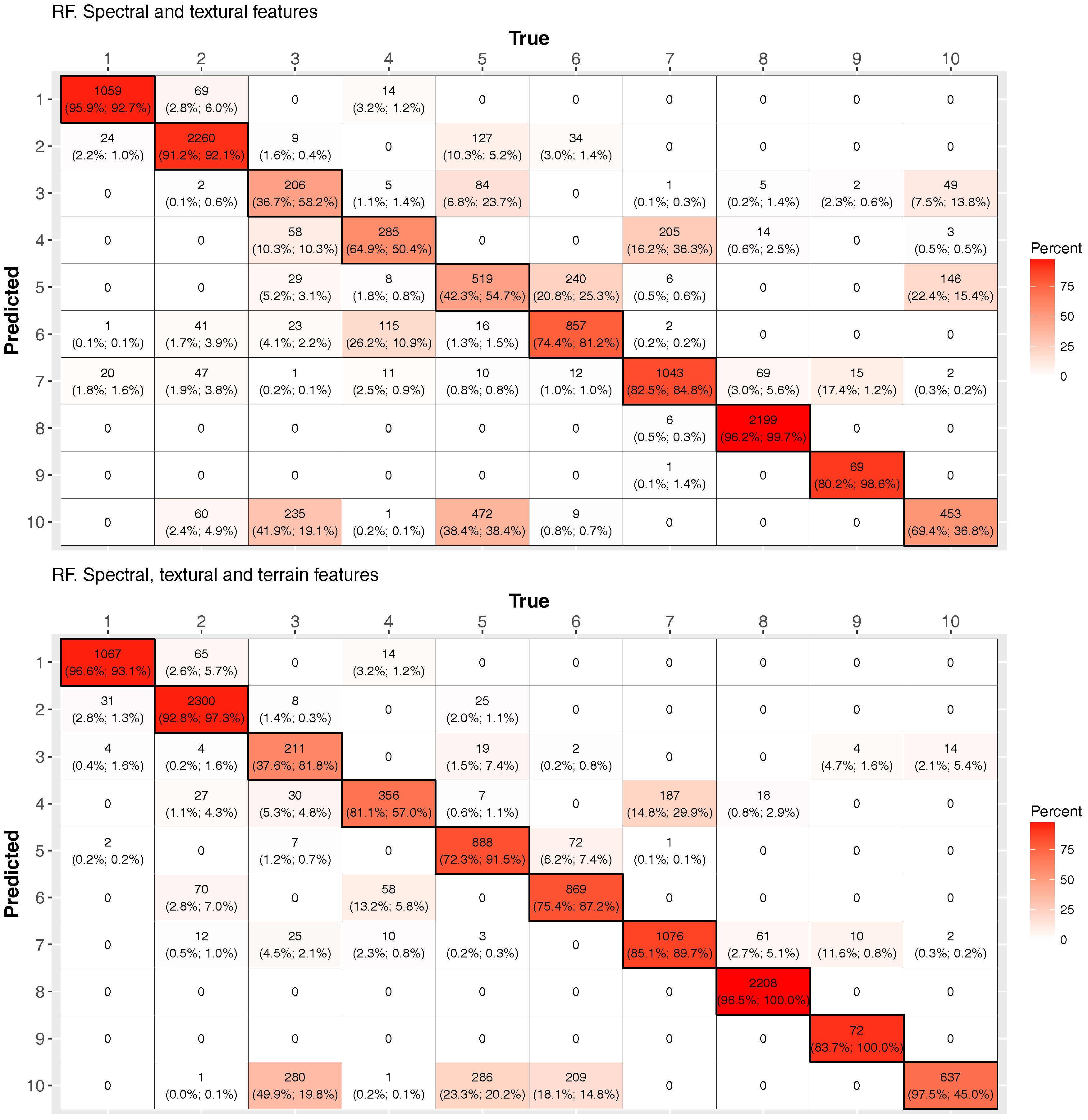
4.4. Per Class Validation

Figure 9 summarizes user’s and producer’s accuracy values for each feature combination and algorithm used in the time series. The classes that correspond to natural vegetation (forest and scrub) are classified more accurately than other classes in almost all cases (kappa around 0.9 or higher) and show less dispersion (M = 94.29%, SD = 2.26%). These two natural vegetation classes are frequently confused. In both cases, the best classifier seems to be SMAP with spectral and textural features (M = 95.09%, SD = 3.26%), although the differences are very small.

Figure 10 shows the confusion matrix for 2015. In the diagonal, the number of correctly classified pixels and the user’s (left) and producer’s (right) accuracy values are represented. The remaining cells show misclassified pixels, the percentage of pixels of one class incorrectly assigned to other classes and the percentage of pixels incorrectly assigned to the class analyzed. The color gradient reflects the average of both percentages.

Natural uses (forest and scrub) and water are the most accurately classified land uses with a reduction in error when relief features are included. The maximum confusion appears among classes that are similar, both in terms of reflectivity and in terms of agronomic properties. For instance, when using the three feature sets, RF classifies almost 50% of the rainfed tree crops as vineyard; indeed, the former is the class least accurately classified in most of the classifications. This sort of confusion appears especially in the surroundings of Elda and Villena (Figure 11, bottom) and produces an overestimation of vineyards. The inclusion of new features does not contribute to the accuracy. The best option to classify this class is SMAP with three feature sets, followed by SMAP with spectral and textural features.

Irrigated tree crops have higher user’s and producer’s accuracy values than the above class (M = 76.04%, SD = 6.99% in the case of irrigated tree crops, M = 45.53%, SD = 9.48% in the case of rainfed tree crops). They also present less dispersion, especially the producer’s accuracy. When analyzing user’s accuracy, it is clear that SMAP and ML provide more accurate values (M = 85.7%, SD = 9.13% in the case of SMAP and M = 88.87%, SD = 7.67% in the case of ML), whereas RF’s and SVM’s accuracies are worse (M = 78.55%, SD = 15.74% and M = 74.6%, SD = 12.19%, respectively), except when using terrain features, when the values are M = 88.57%, SD = 15.51% in the case of RF. RF also benefits from the inclusion of terrain features (SVM only in user’s accuracy), and ML producer’s accuracy is reduced when terrain features are included. Confusion occurs with irrigated grass crops and, to a lesser extent, with rainfed tree crops and rainfed grass crops. As a whole, RF with the three feature sets produces the most accurate classification followed by ML with spectral and textural features.

Another frequent confusion is the misclassification of impervious surfaces as irrigated tree crops. The mixing of both uses is frequent in orchard landscapes near the Mediterranean coast. This fact and the high spectral variability of urban land use explain this confusion.

Rainfed grass crops have, in general, low producer’s accuracy values (M = 49.11%, SD = 12.6%) and high user’s accuracy (M = 77.75%, SD = 11.99%). Confusion tends to occur with irrigated grass crops and, to a lesser extent, with rainfed tree crops and vineyards. All methods increase user’s accuracy when adding new feature sets, but only ML and RF do the same with producer’s accuracy, while SMAP clearly reduces accuracy. In general, the best option is ML with the three feature sets followed by SMAP with spectral and textural features.

Irrigated grass crops (including orchard areas) is a heterogeneous class that reaches quite high accuracy values (M = 73.3%, SD = 7.9% for producer’s accuracy and M = 82.27%, SD = 7.08% for user’s accuracy). All methods improve both accuracies when new features are included. Confusion occurs with the class rainfed grass crops and, to a lesser extent, with irrigated tree crops and rainfed tree crops. RF with the three feature sets is, in general, the best classification option followed by SMAP or ML with spectral and textural features.

Impervious surfaces (buildings and infrastructures) are classified with high accuracy (M = 88.86%, SD = 6.89% in user’s and producer’s accuracy). However, of interest are the SMAP lower user’s accuracy values (M = 66.29%, SD = 17.22% and the lower is 32.36%), while all the other methods have values between 70% and 93% (M = 87.58%, SD = 7.47%). Producer’s accuracy is higher, with values above 90%, except for SVM. RF benefits in both accuracies from the inclusion of new feature sets. Confusion occurs with classes like bare soil, irrigated grass crops and rainfed tree crops. The best classification option is RF with the three feature sets (M = 87.73%, SD = 4.91% is user’s and producer’s accuracy). No significant differences appear among algorithms when spectral and textural features are used to classify.

Water surfaces (artificial or natural) show very high user’s and producer’s accuracy values (M = 95.87%, SD = 11.79%), especially RF (M = 99.27%, SD = 0.91%), which reaches 100% with any combination of feature sets. SMAP with spectral and textural features also produces very high accuracy values; in 2010, omission and commission errors reach 100%. Confusion happens mainly with the impervious class.

Bare soil is represented exclusively by a quarry in the south of the study area, the area of which is small compared with the other classes. The user’s accuracy values are high (M = 92.86%, SD = 13.47%) and similar for the different algorithms, increasing when new features are added. The producer’s accuracy is in most cases in the range 60–90% in the case of RF and SVM, and between 11% and 100% in the case of SMAP and ML. Confusion appears with the class impervious and to a lesser extent with rainfed tree crops. In these cases, the best results are reached with ML and SMAP, using just spectral features (M = 92.72%, SD = 5.24% and M = 93.94%, SD = 5.07% in user’s and producer’s accuracy).

Finally, vineyard includes both irrigated and rainfed systems because their separability is very low. This class is easily confused with similar crops, like rainfed tree crops. A high dispersion is observed in accuracy values. Producer’s accuracy is in the range 64.77–82.49% for ML, in the range 85.71–97.55% for RF with the three feature sets and in the range 30.78–94.74% for SMAP with the three feature sets. Confusion appears with the classes rainfed tree crops, rainfed grass crops and irrigated grass crops. The best user’s and producer’s accuracy values are obtained, as a rule, with RF (M = 75.11% =, SD = 15.1%) and SVM (M = 78.88%, SD = 10.81%), whose values improved when terrain features were added. SMAP with spectral and textural features also gives a high accuracy (M = 75.56%, SD = 8.27%).

4.5. Visual Validation

Figure 11 shows the land use maps obtained with RF, using spectral and textural features (top) and spectral, textural and terrain features (bottom) in 2015. Although this is not the year in which the best results were obtained (see Figure 7), the kappa value is still quite high when using spectral, textural and terrain features ($k=0.838$). In addition, it is the most recent year of the series.

SMAP is the classifier that produces the visually poorest result because of a strong overestimation of Class 7 (impervious surfaces), although in some years, such as 2009, it produces a good classification both visually and quantitatively ($k=0.864$).

Some serious errors appear when ML or SMAP are used, since the Santa Pola coastal marshes are classified as urban; both RF and SVM classify this area correctly, although some overestimation of impervious surfaces is observed when including the three feature sets. In the case of RF, we think the reason is that the biased distribution of urban areas in the study area, concentrated in low altitude and low slope sites, might have led RF to misclassify low height cells as urban. In addition, the importance of the variables obtained with RF give much higher importance to relief features than to the spectral or textural features.

In other cases, misclassifications were observed in coastal areas even with the most accurate classifications (Figure 11, bottom), classifying as Class 6 (irrigated grassland) some coastal urban areas (San Juan or Santa Pola) and, at the same time, expanding the urban areas beyond their real limit.

In summary, it is necessary to visually check the classification results to avoid the sort of problems we have mentioned when using very flexible classifiers with a large number of features.

5. Conclusions

Using images from several seasons significantly improves accuracy, as the differences in the phenological calendars of different land covers are taken into account; however, there are no significant differences between using two or more images. When classifying only one image per year, summer is the best option, probably due to strong differences in the water content between irrigated and non-irrigated covers.

Parameter optimization in RF and SVM does not improve accuracy significantly, but greatly increased the computing time. However, it may be interesting to try other more “expensive” methods of calibration, such as a simultaneous calibration of parameters in a grid, or to use other resampling methods.

Adding textural features to the spectral features does not increase accuracy significantly, but when terrain features are also added, there is a significant increase in accuracy.

SMAP is significantly less accurate than ML, RF or SVM, none of which significantly differ in terms of accuracy. However, the interaction between feature sets and algorithm produces a significant increase in RF accuracy over SVM and ML when terrain features are added. We believe that the good accuracy of ML is partly due to the restrictions taken into account when the training and validation areas are identified and to outlier elimination.

Although some algorithms and feature subsets perform better overall, the results are not so clear when individual classes are analyzed. Some classes benefit from the inclusion of additional feature sets, but others do not. This may indicate that the combined use of different algorithms (depending on individual classes) can be a good line to follow to get better results. Similarly, it may be interesting to use different combinations of strategies depending on the class of interest. Thus, the variables derived from the DEM should not be used in classes such as urban, while it may be a good strategy for use with natural classes such as forest or scrub.

Water surfaces, forest and scrub are the most accurately classified land use. The problem arises with crops, especially with sparse tree crops, mostly in rainfed land. In this case, the greatest confusion occurred with vineyards due to the similar characteristics of both uses. Confusion errors were also detected in rainfed grass crops, especially errors of commission, almost always resulting in confusion with other crops, especially irrigated grass crops.

References

- Alrababah, M.; Alhamad, M. Land use/cover classification of arid and semi-arid Mediterranean landscapes using Landsat ETM. Int. J. Remote Sens. 2006, 27, 2703–2718. [Google Scholar] [CrossRef]
- Di Palma, F.; Amato, F.; Nolè, G.; Martellozzo, F.; Murgante, B. A SMAP Supervised Classification of Landsat Images for Urban Sprawl Evaluation. ISPRS Int. J. Geoinform. 2016, 5, 109. [Google Scholar] [CrossRef]
- Berberoglu, S.; Curran, P.; Lloyd, C.; Atkinson, P. Texture classification of Mediterranean land cover. Int. J. Appl. Earth Obs. Geoinform. 2007, 9, 322–334. [Google Scholar] [CrossRef]
- Senf, C.; Leitão, P.J.; Pflugmacher, D.; Van der Linden, S.; Hostert, P. Mapping land cover in complex Mediterranean landscapes using Landsat: Improved classification accuracies from integrating multi-seasonal and synthetic imagery. Remote Sens. Environ. 2015, 156, 527–536. [Google Scholar] [CrossRef]
- Maselli, F.; Conese, C.; Petkov, L.; Resti, R. Inclusion of prior probabilities derived from a nonparametric process into the maximum likelihood classifier. Photogramm. Eng. Remote Sens. 1992, 58, 201–207. [Google Scholar]
- Breiman, L. Random Forests. Mach. Learn. 2001, 45, 5–32. [Google Scholar] [CrossRef]
- Cortes, C.; Vapnik, V. Support-vector network. Mach. Learn. 1995, 20, 1–5. [Google Scholar] [CrossRef]
- McCauley, J.; Engel, B. Comparison of scene segmentations: SMAP, ECHO, and maximum likelihood. IEEE Trans. Geosci. Remote Sens. 1995, 33, 1313–1316. [Google Scholar] [CrossRef]
- Ehsani, A. Evaluation of sequential maximum a posteriori (SMAP) Method for Land Cover Classification. In Proceedings of the Geomatics 90 (National Conference & Exhibition), Tehran, Iran, 30 May–1 June 2011. [Google Scholar]
- Li, M.; Im, J.; Beier, C. Machine learning approaches for forest classification and change analysis using multi-temporal Landsat TM images over Huntington Wildlife Forest. GISci. Remote Sens. 2013, 50, 361–384. [Google Scholar]
- Sluiter, R.; Pebesma, E.J. Comparing techniques for vegetation classification using multi- and hyperspectral images and ancillary environmental data. Int. J. Remote Sens. 2010, 31, 6143–6161. [Google Scholar] [CrossRef]
- He, J.; Harris, J.; Sawada, M.; Behnia, P. A comparison of classification algorithms using Landsat-7 and Landsat-8 data for mapping lithology in Canada’s Arctic. Int. J. Remote Sens. 2015, 36, 2252–2276. [Google Scholar] [CrossRef]
- Rodríguez-Galiano, V. Metodología Basada en Teledetección, SIG Y Geoestadística Para Cartografía Y Análisis De Cambios De Cubiertas Del Suelo De La Provincia De Granada. Ph.D. Thesis, Department of Geodynamics, University of Granada, Granada, Spain, 2011. [Google Scholar]
- Rodriguez-Galiano, V.; Ghimire, B.; Rogan, J.; Chica-Olmo, M.; Rigol-Sanchez, J. An assessment of the effectiveness of a random forest classifier for land-cover classification. ISPRS J. Photogramm. Remote Sens. 2012, 67, 93–104. [Google Scholar] [CrossRef]
- Belgiu, M.; Drăguţ, L. Random forest in remote sensing: A review of applications and future directions. ISPRS J. Photogramm. Remote Sens. 2016, 114, 24–31. [Google Scholar] [CrossRef]
- Ehsani, A.; Quiel, F. Efficiency of Landsat ETM+ Thermal Band for Land Cover Classification of the Biosphere Reserve “Eastern Carpathians” (Central Europe) Using SMAP and ML Algorithms. Int. J. Environ. Res. 2010, 4, 741–750. [Google Scholar]
- Kumar, U.; Dasgupta, A.; Mukhopadhyay, C.; Ramachandra, T. Advanced Machine Learning Algorithms based Free and Open Source Packages for Landsat ETM+ Data Classification. In Proceedings of the OSGEO-India: FOSS4G 2012- First National Conference: Open Source Geospatial Resources to Spearhead Development and Growth, Andhra Pradesh, India, 25–27 October 2012; pp. 1–7. [Google Scholar]
- Elumnoh, A.; Shrestha, R. Application of DEM data to Landsat image classification: Evaluation in a tropical wet-dry landscape of Thailand. Photogramm. Eng. Remote Sens. 2000, 66, 297–304. [Google Scholar]
- Lu, D.; Weng, Q. A survey of image classification methods and techniques for improving classification performance. Int. J. Remote Sens. 2007, 28, 823–870. [Google Scholar] [CrossRef]
- Zhou, Q.; Robson, M. Contextual information is ultimately necessary if one is to obtain accurate image classifications. Int. J. Remote Sens. 2001, 22, 612–625. [Google Scholar]
- Eisavi, V.; Homayouni, S.; Yazdi, A.M.; Alimohammadi, A. Land cover mapping based on random forest classification of multitemporal spectral and thermal images. Environ. Monit. Assess. 2015, 187, 187–291. [Google Scholar] [CrossRef] [PubMed]
- Gómez, C.; White, J.C.; Wulder, M.A. Optical remotely sensed time series data for land cover classification: A review. ISPRS J. Photogramm. Remote Sens. 2016, 116, 55–72. [Google Scholar] [CrossRef]
- CHJ. Plan Hidrológico de la Demarcación Hidrográfica del Júcar; Technical Report; Cemarcación Hidrográfica del Júcar, Ministerio de Medio Ambiente: Singapore, 2015. [Google Scholar]
- Bossard, M.; Feranec, J.; Otahel, J. CORINE Land Cover Technical Guide - Addendum 2000; Technical Report No. 40; European Environment Agency: Copenhagen, Denmark, 2000. [Google Scholar]
- Chávez, P. An improved dark-object substraction technique for atmospheric scattering correction of multispectral data. Remote Sens. Environ. 1988, 24, 459–479. [Google Scholar] [CrossRef]
- Teillet, P.; Guindon, B.; Goodenough, D. On the slope-aspect correction of multispectral scanner data. Can. J. Remote Sens. 1982, 8, 84–106. [Google Scholar] [CrossRef]
- Swain, P.; Davis, S.E. Remote Sensing: The Quantitative Approach; McGraw-Hill: New York, NY, USA, 1976; p. 396. [Google Scholar]
- Liaw, A.; Wiener, M. Classification and Regression by randomForest. R News 2002, 2, 18–22. [Google Scholar]
- Gislason, P.; Benediktsson, J.; Sveinsson, J. Random Forests for land cover classification. Pattern Recognit. Lett. 2006, 27, 294–300. [Google Scholar] [CrossRef]
- Ghimire, B.; Rogan, J.; Miller, J. Contextual land-cover classification: Incorporating spatial dependence in land-cover classification models using random forests and the Getis statistic. Remote Sens. Lett. 2010, 1, 45–54. [Google Scholar] [CrossRef]
- Pal, M. Random forest classifier for remote sensing classification. Int. J. Remote Sens. 2005, 26, 217–222. [Google Scholar] [CrossRef]
- Prasad, A.; Iverson, L.; Liaw, A. Newer Classification and Regression Tree Techniques: Bagging and Random Forests for Ecological Prediction. Ecosystems 2006, 9, 181–199. [Google Scholar] [CrossRef]
- Cutler, D.; Edwards, T., Jr.; Beard, K.; Cutler, A.; Hess, K.; Gibson, J.; Lawler, J. Random forest for classification in ecology. Ecology 2007, 88, 2783–2792. [Google Scholar] [CrossRef] [PubMed]
- Cánovas-García, F.; Alonso-Sarría, F.; Gomariz-Castillo, F.; Onate Valdivieso, F. Modification of the random forest algorithm to avoid statistical dependence problems when classifying remote sensing imagery. Comput. Geosci. 2017, 103, 1–11. [Google Scholar] [CrossRef]
- Hastie, T.; Tibshirani, R.; Friedman, J. The Elements of Statistical Learning: Data Mining, Inference, and Prediction, 2nd ed.; Springer: Berlin, Germany, 2009. [Google Scholar]
- Camps-Valls, G.; Bruzzone, L. (Eds.) Kernel Methods for Remote Sensing Data Analysis, 1st ed.; John Wiley & Sons, Ltd.: Chichester, UK, 2009. [Google Scholar]
- Mountrakis, G.; Im, J.; Ogole, C. Support vector machines in remote sensing: A review. ISPRS J. Photogramm. Remote Sens. 2011, 66, 247–259. [Google Scholar] [CrossRef]
- Vapnik, V. Statistical Learning Theory, 1st ed.; Wiley Interscience: Hoboken, NJ, USA, 1998; p. 736. [Google Scholar]
- Gualtieri, J.; Cromp, R. Support Vector Machines for Hyperspectral Remote Sensing Classification. In Proceedings of the 27th AIPR Workshop: Advances in Computer Assisted Recognition, Washington, DC, USA, 14–16 October 1998. [Google Scholar]
- Melgani, F.; Bruzzone, L. Classification of hyperspectral remote sensing images with support vector machines. IEEE Trans. Geosci. Remote Sens. 2004, 42, 1778–1790. [Google Scholar] [CrossRef]
- Tso, B.; Mather, P. Classification Methods for Remotely Sensed Data, 2nd ed.; Taylor & Francis: Didcot, UK; Abingdon, UK, 2009; p. 352. [Google Scholar]
- Auria, L.; Moro, R. Support Vector Machines (SVM) as a Technique for Solvency Analysis; Discussion Papers of DIW Berlin 811; German Institute for Economic Research: Berlin, Germany, 2008. [Google Scholar]
- Bouman, C.; Shapiro, M. Multispectral Image Segmentation using a Multiscale Image Model. In Proceedings of the IEEE International Conference on Acoustic, Speech and Signal Processing, San Francisco, CA, USA, 23–26 March 1992; pp. III565–III568. [Google Scholar]
- Bouman, C.; Shapiro, M. A Multiscale Random Field Model for Bayesian Image Segmentation. IEEE Trans. Image Process. 1994, 3, 162–177. [Google Scholar] [CrossRef] [PubMed]
- Cheng, H.; Bouman, C.A. Multiscale Bayesian Segmentation Using a Trainable Context Model. IEEE Trans. Image Process. 2001, 10, 511–525. [Google Scholar] [CrossRef] [PubMed]
- Mather, P.; Koch, M. Computer Processing of Remotely-Sensed Images: An Introduction, 4th ed.; Wiley: Hoboken, NJ, USA, 2010. [Google Scholar]
- Molinaro, A.; Simon, R.; Pfeiffer, R. Prediction error estimation: A comparison of resampling methods. Bioinformatics 2005, 21, 3301–3307. [Google Scholar] [CrossRef] [PubMed]
- Kuhn, M.; Johnson, K. Over-Fitting and Model Tuning. In Applied Predictive Modeling; Springer: New York, NY, USA, 2013; pp. 61–92. [Google Scholar]
- Caputo, B.; Sim, K.; Furesjo, F.; Smola, A. Appearance-based object recognition using SVMS: Which kernel should I use? In Proceedings of the NIPS Workshop on Statitsical Methods for Computational Experiments in Visual Processing and Computer Vision, Whistler, BC, Canada, 12–14 December 2002. [Google Scholar]
- Karatzoglou, A.; Smola, A.; Hornik, K.; Zeileis, A. kernlab—An S4 Package for Kernel Methods in R. J. Stat. Softw. 2004, 11, 1–20. [Google Scholar] [CrossRef]
- Breiman, L.; Friedman, J.; Olshen, R. Classification and Regression Trees. 1984. Available online: https://pdfs.semanticscholar.org/df5a/9aeb6ad2ebda81afc7e0377bcd770a3c19f9.pdf (accessed on 17 October 2017).
- Neteler, M.; Mitasova, H. Open Source GIS. A GRASS GIS Approach, 3rd ed.; The International Series in Engineering and Computer Science; Springer: New York, NY, USA, 2008; Volume 773, p. 486. [Google Scholar]
- Neteler, M.; Bowman, M.; Landa, M.; Metz, M. GRASS GIS: A multi-purpose open source GIS. Environ. Model. Softw. 2012, 31, 124–130. [Google Scholar] [CrossRef]
- Venables, W.; Smith, D. The R Development Core Team. In An Introduction to R; 2012; Available online: http://www.math.vu.nl/stochastics/onderwijs/statlearn/R-Binder.pdf (accessed on 17 October 2017).
- R Core Team. R: A Language and Environment for Statistical Computing; R Foundation for Statistical Computing: Vienna, Austria, 2012. [Google Scholar]
- Cohen, J. A coefficient of agreement for nominal scales. Educ. Psychol. Meas. 1960, 20, 37–46. [Google Scholar] [CrossRef]
- Congalton, R.; Mead, R. A Quantitative Method to Test for Consistency and Correctness in Photointerpretation. Photogramm. Eng. Remote Sens. 1983, 49, 69–74. [Google Scholar]
- Chuvieco, E. Fundamentals of Satellite Remote Sensing. An Environmental Approach; CRC Press: Boca Raton, FL, USA, 2016. [Google Scholar]
- Landis, J.; Koch, G. The Measurement of Observer Agreement for Categorical Data. Biometrics 1977, 33, 159–174. [Google Scholar] [CrossRef] [PubMed]
- Congalton, R.; Green, K. Assessing the Accuracy of Remotely Sensed Data: Principles and Practices; Mapping Science, Taylor & Francis: Didcot, UK; Abingdon, UK, 1998. [Google Scholar]
- Long, J.; Ervin, L. Using Heteroscedasticity Consistent Standard Errors in the Linear Regression Model. Am. Stat. 2000, 54, 217–224. [Google Scholar]