Improving Jason-2 Sea Surface Heights within 10 km Offshore by Retracking Decontaminated Waveforms
by
 , , and
Zhengkai Huang
1,2, 
Haihong Wang
1,3,*,
Zhicai Luo
4,
C. K. Shum
5,6,
Kuo-Hsin Tseng
7,8,9 and
Bo Zhong
1,3 
1
School of Geodesy and Geomatics, Wuhan University, Wuhan 430079, China
2
Guangxi Key Laboratory of Spatial Information and Geomatics, Guilin University of Technology, Guilin 541004, China
3
Key Laboratory of Geospace Environment and Geodesy, Ministry of Education, Wuhan University, Wuhan 430079, China
4
MOE Key Laboratory of Fundamental Physical Quantities Measurement, School of Physics, Huazhong University of Science and Technology, Wuhan 430074, China
5
Division of Geodetic Science, School of Earth Sciences, Ohio State University, Columbus, OH 43210, USA
6
State Key Laboratory of Geodesy and Earth’s Dynamics, Institute of Geodesy and Geophysics, Chinese Academy of Sciences, Wuhan 43077, China
7
Department of Civil Engineering, National Central University, Taoyuan 32001, Taiwan
8
Center for Space and Remote Sensing Research, National Central University, Taoyuan 32001, Taiwan
9
Institute of Hydrological and Oceanic Sciences, National Central University, Taoyuan 32001, Taiwan
*
Author to whom correspondence should be addressed.
Remote Sens. 2017, 9(10), 1077; https://doi.org/10.3390/rs9101077
Submission received: 7 June 2017
/
Revised: 5 October 2017
/
Accepted: 19 October 2017
/
Published: 23 October 2017
(This article belongs to the Special Issue Satellite Altimetry for Earth Sciences)
Abstract
:It is widely believed that altimetry-derived sea surface heights (SSHs) in coastal zones are seriously degraded due to land contamination in altimeter waveforms from non-marine surfaces or due to inhomogeneous sea state conditions. Spurious peaks superimposed in radar waveforms adversely impact waveform retracking and hence require tailored algorithms to mitigate this problem. Here, we present an improved method to decontaminate coastal waveforms based on the waveform modification concept. SSHs within 10 km offshore are calculated from Jason-2 data by a 20% threshold retracker using decontaminated waveforms (DW-TR) and compared with those using original waveforms and modified waveforms in four study regions. We then compare our results with retracked SSHs in the sensor geophysical data record (SGDR) and with the state-of-the-art PISTACH (Prototype Innovant de Système de Traitement pour les Applications Côtières et l’Hydrologie) and ALES (Adaptive Leading Edge Subwaveform) products. Our result indicates that the DW-TR is the most robust retracker in the 0–10 km coastal band and provides consistent accuracy up to 1 km away from the coastline. In the four test regions, the DW-TR retracker outperforms other retrackers, with the smallest averaged standard deviations at 15 cm and 20 cm, as compared against the EGM08 (Earth Gravitational Model 2008) geoid model and tide gauge data, respectively. For the SGDR products, only the ICE retracker provides competitive SSHs for coastal applications. Subwaveform retrackers such as ICE3, RED3 and ALES perform well beyond 8 km offshore, but seriously degrade in the 0–8 km strip along the coast.
1. Introduction
Satellite radar altimetry is a powerful technology for remotely sensing physical properties of global oceans. Sea surface heights (SSHs) are the primary product of altimetry, which have greatly benefited studies of extensive scientific issues in geodesy, oceanography, geophysics and many other disciplines [1]. Despite the remarkable success of altimetry in the open ocean, which can provide SSHs with an accuracy of several centimeters, altimetry-derived SSHs in coastal zones are severely degraded due to inherent limitations of this technique [2,3,4]. The Altimeter emits pulse-limited radar signals and receives echoes from illuminated Earth surfaces in nadir. The distance from satellite to the sea surface covered by the radar footprint, referred to as the range, is measured by tracking the received waveform. Hence, SSH can be derived by subtracting the range from satellite altitude. In coastal zones, altimeter waveforms show diversely complex shapes because of land in the footprint and complicated sea state conditions [5,6]. In this case, erroneous range measurements might be delivered by on-board retrackers, which are designed for normal waveforms in the open ocean. In addition, inaccurate media and geophysical corrections such as atmospheric delay corrections, tides, sea state bias (SSB), etc., are non-negligible factors for the poor quality of coastal SSHs [7,8,9]. These corrections are more complex near the coast and it is considerably more difficult to improve them.
Coastal regions play a very important role in the geographical and economical support of human society, and therefore the coastal environment is subject to great pressure from human activities [10]. High quality and dense sampling of geospatial and environmental information is expected not only for coastal management but also for scientific research, e.g., [11]. The increasing demands of coastal applications have motivated excellent efforts in the altimetry community to improve coastal applicability, including proposing new altimetry concepts (Ka-band altimetry [12], delay-Doppler altimetry [13,14], wide-swath altimetry [15], GNSS altimetry [16], constellations of altimeters [17]) and reprocessing conventional altimeter data [18,19,20]. In the last decade, a series of projects were supported by some space agencies and research institutions, aiming to retrieve valid altimeter data as close as possible to the coast. Hereafter a few data sets have been available for coastal applications, such as PISTACH (Prototype Innovant de Système de Traitement pour les Applications Côtières et l’Hydrologie) as well as coastal and hydrology altimetry data products [21], COASTALT [22] and X-TRACK [23]. There is increasing consensus that coastal altimetry is a critically important yet challenging discipline.
The endeavor in coastal altimetry consists of refining auxiliary corrections and retracking waveforms [4,20], which are performed to tackle the aforementioned factors degrading conventional altimeter data near the coasts. A summary of the significant achievements was given in [24], including improvements in waveform retracking, tropospheric corrections, tide models, and dynamic atmosphere corrections. There are also some studies on SSB correction, aiming at better modelling the error induced by ocean surface waves, whitecaps and foam [25,26,27,28,29]. Among these improvements, waveform retracking is getting considerable attention in recent years, because of its evident effect on the enhancement of altimeter measurements.
The waveform retracking technique was originally designed for post-processing open ocean radar waveforms. The Brown mathematical model [30] is used to fit ocean waveforms in order to refine parameters related to reflective surfaces, referred to as OCEAN retracker. For waveforms over mixed surfaces, a threshold retracker (TR) was developed [31] for specular or multi-peak shapes. This approach determines retracked gate using a preset percentage of maximum echo power. Later, several revised algorithms based on TR were proposed for coastal applications, and successfully validated in some case studies. For instance, Hwang et al. [32] presented an improved threshold retracker (ITR) and verified better performance than the OCEAN and TR methods using Geosat geodetic mission (GM) altimeter data around Taiwan. Another modified threshold retracker (MTR) was applied to Jason-2 data over California coastal ocean, which could filter the pre-leading edge bumps [33]. This kind of retracker extracts subwaveform in order to avoid superimposed signals from non-marine surfaces by detecting the apparent leading edge. Similarly, assuming waveforms contain a portion unaffected by land effects, a series of subwaveform retrackers have been developed [34,35,36,37,38]. Some other approaches that use refined model-based retrackers, such as Brown plus specular peak model [39] and the Brown with asymmetric Gaussian peak (BAGP) model [6], were developed to conform peaky altimetric waveforms that occupy a large percentage of coastal areas. In addition, some researchers developed adaptive retracking systems by applying an optimal retracker for various characteristic shapes, on the basis of waveform classification [36,38,40,41,42]. Although these retrackers contribute enormously to coastal SSH retrievals with better accuracy and shortened coastal gaps, handling coastal waveforms within 10 km of the shore is still a thorny issue [2,38,43].
The major obstacle for coastal waveform retracking is due to the diversity and complexity of coastal waveforms. According to the classification of the coastal waveforms within PISTACH processing [21], the percentage of typical ocean waveforms starts decreasing around 10 km away from the coast, whilst the quantity of waveforms with the shape of the Brown plus anomalous peaks rapidly increases. More than a quarter of the waveforms do not obey the Brown model at the distance of 8 km off the shoreline [6]. Within 5 km away from the shoreline, the peaky waveforms outnumber the ocean waveforms. Anomalous peaks in waveforms might cause an overestimation of some waveform parameters for empirical retrackers or make model-based retracker failure. In order to purify waveforms, a waveform modification (WM) concept was presented by Tseng et al. [43]. In their study, they proposed an algorithm to modify polluted coastal waveforms before retracking. By retracking modified waveforms, it was demonstrated in four cases in North America that SSHs in 1–7 km coastal zone had smaller root mean square error (RMSE) than those from retracking original waveforms, comparing with the in-situ tide gauge data. However, shifted leading edges might be misjudged as spurious peaks and then distorted in their procedure, if the selected reference waveform is not representative (further discussion given in Section 3.1). Another issue is that an interpolation for amending outlier gates might induce noise from adjacent gates.
In this paper, an alternative strategy for decontaminating waveforms is presented in order to overcome these defects of the WM method. We revise the criterion for selecting reference waveforms, and directly set the outliers as null value rather than amending them by interpolation, i.e., the detected spurious gates would not be taken into consideration in the retracking procedure. The performance of this new approach is evaluated in four coastal regions within 10 km offshore using Jason-2 data. The article is structured as follows. The study regions and dataset used in the present study are described in Section 2. In Section 3, the WM method is reviewed and a modified algorithm is proposed. The strategy for computation and evaluation of the retracked SSHs is also introduced in this section. The retracked SSHs by various retrackers are validated using geoidal heights and tide gauge data in Section 4. Further discussions about our results are presented in Section 5. Finally, some conclusions and recommendations are summarized in Section 6.
2. Materials and Study Regions
2.1. Jason-2 Altimeter Data
The Ocean Surface Topography Mission (OSTM)/Jason-2 satellite, launched in June 2008, is an international mission between the National Aeronautics and Space Administration (NASA), the Central National d’Etudes Spatiales (CNES), the National Oceanic and Atmosphere Administration (NOAA) and the European Organization for the Exploitation of Meteorological Satellites (EUMETSAT). One vital objective of Jason-2 is to extend the time series of SSH observations beyond TOPEX/Poseidon (T/P) and Jason-1 by more than two decades. As a successor to T/P and Jason-1, Jason-2 not only inherited the characteristics of its predecessors: a similar payload (Poseidon altimeter) and an identical orbit (inclination: ~66°; revisit period: ~10 days), but also made some improvements in instruments, data processing and algorithms. For instance, the Poseidon-3 altimeter on Jason-2 has a lower instrumental noise and adopts a better tracking algorithm for land and ice surface than preceding generations of Poseidon altimeters [44]. These improvements are expected to increase the accuracy of sea surface height measurement to about 2.5 cm [45]. A detailed description of Jason-2 mission is referred to in [46].
The Jason-2 sensor geophysical data record (SGDR) product version d (JA2-GPS-PdP) provided by AVISO (Archiving, Validation and Interpretation of Satellite Oceanographic data)/CNES was used in this study. This dataset is a reprocessed delivery product, containing waveforms and all relevant corrections needed to retrieve SSHs. The waveform information is required for ground post-processing (i.e., retracking). Originally, the Jason-2 altimeter receives about 2060 elementary echoes per second. In order to reduce the thermal and speckle noise, waveforms are produced at a 20 Hz rate by averaging elementary echoes over 50 ms on board [44]. Detailed description of waveform sampling is suggested to refer [47]. Each waveform in SGDR comprises 104 sampling gates with an on-board tracking gate at #32.5. In addition to the operating tracker ranges, three types of retracked ranges calculated by OCEAN (MLE4), MLE3, and ICE retrackers, are included in SGDR [48].
For comparison, we employed the coastal and hydrology altimetry products released by the Collecte Localisation Satellites (CLS) in the frame of the PISTACH project. The PISTACH project is funded by CNES, aiming to improve Jason-2 altimetry data over coastal areas and continental waters. The PISTACH products are divided into two categories: one for coastal applications and the other for hydrology. Coastal products cover the whole ocean and a 25-km fringe over land. Hydrology products cover all continents plus a 25-km band over coastal ocean. Four alternative ranges are available in PISTACH products, namely, ICE1, ICE3, RED3 and OCE3 [21]. Therein, the ICE1 retracker, as well as the ICE retracker in SGDR, is based on the Offset Center of Gravity (OCOG) method [49], which determines range epoch by the first sample in which power is larger than 30% of the COG amplitude. The ICE3 retracker has the same principle as the ICE1 retracker, but only part of the samples around the main leading edge is taken into computation. The RED3 method retracks parameters with a maximum likelihood estimator in a small window selected in the same way as ICE3 retracker. The OCE3 range is obtained by applying the classical MLE3 retracker to filtered waveforms by singular value decomposition filtering.
2.2. Study Regions
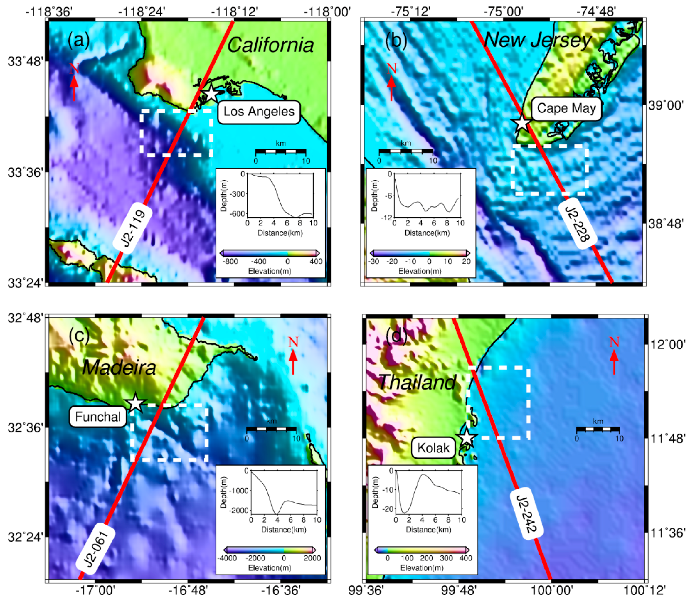
Four study regions with different relief and sea state conditions were selected in order to evaluate the SSHs retrieved by various retrackers (Figure 1). Characteristics of the coast have a great effect on the shape of altimeter waveforms [50]. Complex topography will decrease the amount of recognizable waveforms in the coast area. Region (a) is located near the NOAA gauge station in Los Angeles, west coast of US. Ocean bottom elevation has a sudden drop near to 5 km offshore, with a relatively smooth slope between 0–4 km and 6–10 km. Region (b), neighboring to Cap May at the east coast of US, has the most gradual variation in topography and the shallowest water depth among the four study regions. Region (c) is at the south of Madeira Island, Portugal. In this region, the coastal topography is composed of a mountain ridge and the ocean depth sharply drops by 2000 m within 4 km. In contrast, water depth is also very shallow (<22 m) in region (d). Different from other regions, region (d) has a small angle between satellite track and coastline, which lengthens the effect of land contamination and results in a great number of waveforms deviating from the Brown model.
In each study region, there is a Jason-2 pass and a vicinal tide gauge station. These four track segments used in this study consist of two approaching and two leaving land, corresponding to ascending and descending passes respectively. The flight direction of the satellite is denoted by the orientation of the pass tag in Figure 1. A brief introduction to the Jason-2 data used in the four study locations is given in Table 1. Cycles of altimeter data used in the study are selected according to the time span of available gauge data. The tide gauge data are downloaded from the University of Hawaii Sea Level Center (UHSLC). The hourly research quality data are used, which are the final science-ready dataset released 1–2 years after raw data are received by UHSLC [52].
3. Methodologies
3.1. Recapitulation of the WM Technique
WM is a statistical approach to trim off anomalous peaks of land contamination in the stacked waveforms [43]. An empirical criterion is exploited to detect the spurious peaks, and then the corresponding gates are amended by a 2-D interpolation from neighboring nodes. Firstly, the averaged waveform over deeper oceans is calculated as a reference waveform for each pass. Secondly, the residual waveform is defined as the following Equation (1), i.e., subtracting the reference from the original waveform.
where are the n-th original waveform and the corresponding residual, is the reference waveform. If the i-th gate value in the residual waveform fulfills the criterion given in Equation (2), the original waveform sampling related to the i-th gate will be judged as an outlier.
where is the standard deviation of the n-th residual waveform. Finally, the outlier is replaced by the interpolated value from the neighboring samples in the current waveform and its adjacent waveforms.
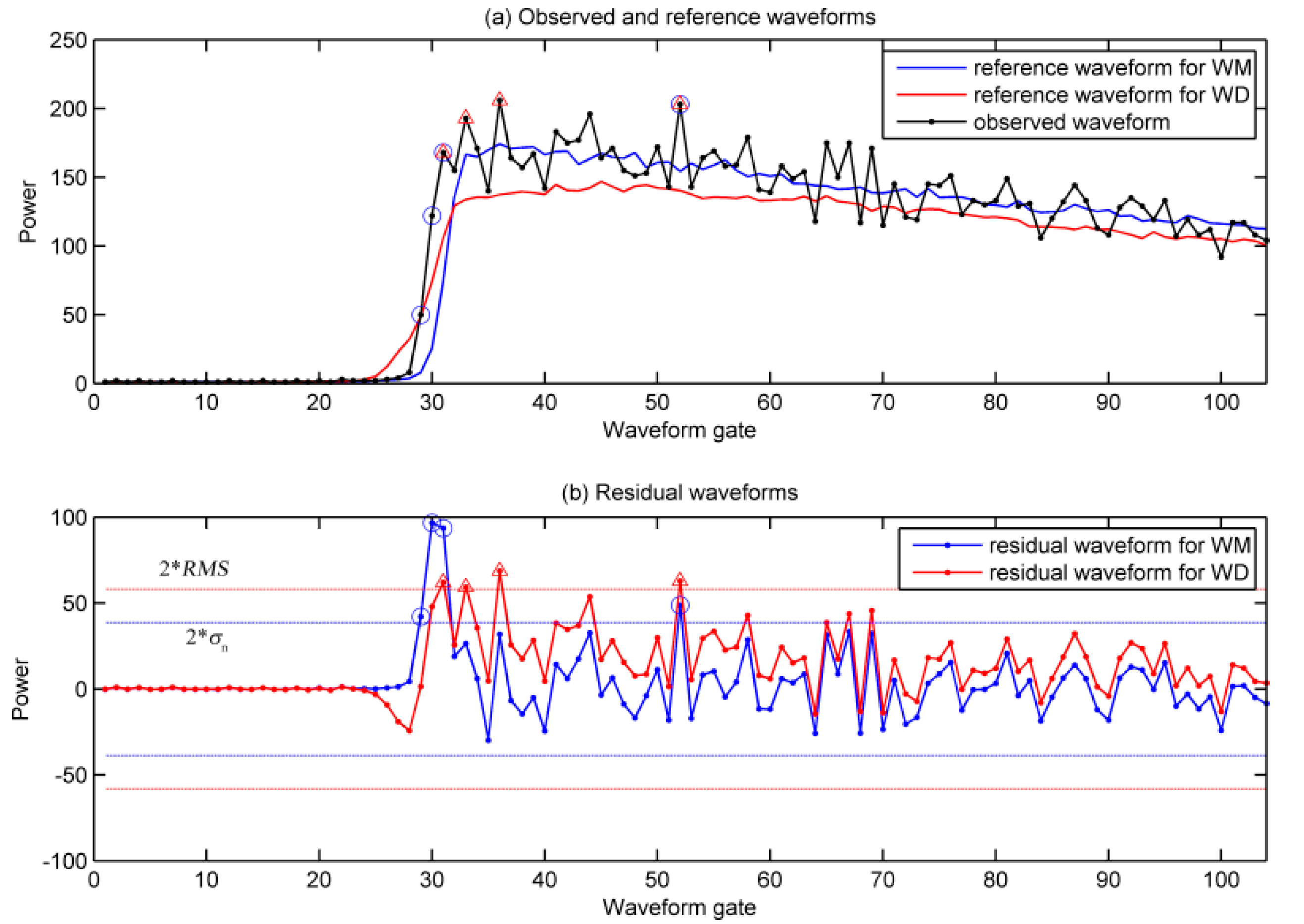
The crucial point of the WM method is the selection of the reference waveform. An averaged waveform within 20–30 km of the coast is treated as an ocean waveform, of which the midpoint of the leading edge is very close to the nominal tracking gate. Tseng et al. [43] used it as the reference to detect spurious gates with contaminations from non-marine surfaces and achieved good results in most cases. However, there is one possibility when the leading edge of the waveform migrates far away from the nominal tracking gate. It often happens in the transition zone between land and sea. In this case, the reference waveform might lose its representativeness and bring about worse results. It can explain why the WM method had no improvement for SSHs within 0.5–1 km of the shoreline. Figure 2 demonstrates a failed case of the WM method near Cape May, NJ, USA, which is also the study region of Case 1 in [43]. It can be seen that original waveforms (Figure 2a) begin to shift at a latitude of 38.83° compared to waveforms over deeper ocean. These waveforms form an apparent bump between 38.85° and 38.90°. The shift causes large residuals near the nominal tracking gate for these waveforms (see Figure 2b) and subsequently misleads the judgment of contaminated gates. The leading edge in modified waveforms would be seriously distorted as a result (Figure 2c).
There is also a potential problem in repairing outliers. Nearby gates of the detected outliers have a high probability of being polluted by land effect, but their amplitudes are not enough to be judged as anomalies. Therefore, interpolation from nearby gates might not completely remove the anomalous peaks.
3.2. Waveform Decontamination
To avoid the abovementioned problems, three revisions for the WM method were made in this study. Here, the revised procedure is referred to as waveform decontamination (WD), to distinguish it from the WM. Firstly, we substituted the averaged waveform within 20 km of the coast as the reference waveform for the mean waveform between 20–30 km. Secondly, the standard deviation () of the individual waveform was replaced with the root mean square (RMS) of all residual waveforms in the study region
where N is the total number of waveforms in the study region, M is the number of waveform sampling gates (104 for Jason-2). By applying the new criterion, spurious gates were detected as in the WM method. Finally, outliers were directly set to null value in our procedure, instead of being repaired in the WM.
The first two revisions make the criterion for outlier detection more tolerant of the waveform shift. This is because the reference waveform and RMS used in the WD contain information of coastal waveforms to be modified, and therefore are more representative of these waveforms than those in the WM. The third revision we made is aiming to avoid errors induced by interpolation. These modifications are helpful to reduce the misjudgment of outliers and the risk of waveform distortion after amending. An example in Figure 3 shows the improvement after these revisions. The leading edge of the observed waveform (black curve with dots in Figure 3a) deviates from that of the reference waveform for the WM (blue curve in Figure 3a). This phase shift causes extreme residuals at two sampling gates on the leading edge (see Figure 3b). Therefore, these gates will be misjudged as anomalous samples by the WM. In contrast, the misjudgment does not happen in the case of the WD. This is because the reference waveform for the WD (red curve in Figure 3a) has a much gentle leading edge, which intersects the leading edge of the observed waveform. Meanwhile, the RMS computed using Equation (3) is larger than used in Equation (2), since the RMS contains contribution from shifted waveforms in the study area.
3.3. Computation and Evaluation of the Retracked SSHs
In order to test the efficiency of the WD method, 20% TR was used to retrack the original waveforms (Ori-TR), modified waveforms (MW-TR) and decontaminated waveforms (DW-TR), respectively. Because the decontaminated waveform may contain null values, traditional formula of TR to determine the retracked gate should be slightly reformed as
where is the retracked gate, is the threshold level, is the first gate with power exceeding , is the first non-null gate before , and are the power at gate and , respectively. The threshold level is computed using
where is the thermal noise which is determined by averaging the power in the first five gates, is the threshold (20% in the present study), is the maximum power of a waveform. Then the retracked range correction is calculated using the offset between the retracked gate and the nominal tracking gate multiplied by the one way range corresponding to the sampling interval.
After waveform retracking correction, the media and geophysical corrections were included to correct range estimations. All atmosphere corrections used in this study were model-derived values. The dry and wet troposphere corrections were calculated using climate models from the European Centre for Medium-range Weather Forecasts (ECMWF). The ionosphere corrections were derived from the Global Ionospheric Maps (GIM). The ocean/solid earth/pole tide corrections were computed using FES2004, Cartwright and Taylor tidal potential, Equilibrium model, respectively [45]. These corrections were provided both in SGDR and in PISTACH. The SSB corrections and the dynamic atmosphere corrections we used in this study were retrieved from the PISTACH product. The SSB corrections associated with OCEAN retracker in PISTACH had the smallest number of default values, and hence were applied to the other retracked SSHs.
Two methods were employed to evaluate the retracked SSHs. First, along-track SSHs were compared to their corresponding geoidal heights derived from EGM2008 model [53]. The standard deviation (SD) of difference between along-track SSHs and geoidal heights was computed, which can be used to assess the variability of the along-track SSHs during each cycle. Second, the SSHs were compared to nearby tide gauge data. In order to evaluate the altimeter-derived SSHs using in-situ sea level, tidal corrections were removed from the SSHs. Selecting the gauge station as the reference point, the SSH time series were determined by correcting the geoid differences between locations of measurements and gauge station. To avoid datum differences between altimeter measurements and in-situ observations, the temporal mean value in the time series was removed. Since the sampling interval of the altimeter-derived SSH time series is only ~10 days, the in-situ sea level was linearly interpolated at each epoch of altimetry observations from the hourly sampling of gauge level data. Finally, the SD and correlation coefficient between altimeter and in-situ time series were computed.
4. Results
In order to retain as many measurements as possible, no data editing was performed on SGDR and PISTACH products. Nine retrackers were compared in this study, including three retrackers (ICE, OCEAN, MLE3) from SGDR, three retrackers (ICE3, OCE3, RED3) from PISTACH, and three retrackers (Ori-TR, MW-TR, DW-TR) performed in this study. Table 2 lists the 20 Hz data availability of various retrackers within 10 km of the shoreline in four study regions. It should be noted that the distance to the coastline was approximately represented by the along-track distance to the point where the satellite ground track crosses the coastline. The data availability rates of OCEAN and OCE3 are very low in the coastal area. OCE3 only successfully retracked 54% waveforms, which is equivalent to the percentage of ocean waveforms classified in PISTACH. In the following discussion, the OCE3 retracker was not taken into account due to its low data availability. It should be clarified that all retrackers were applied to the 0–20 km coastal band, although this study focuses on an area within 10 km offshore.
4.1. Comparison to Geoid
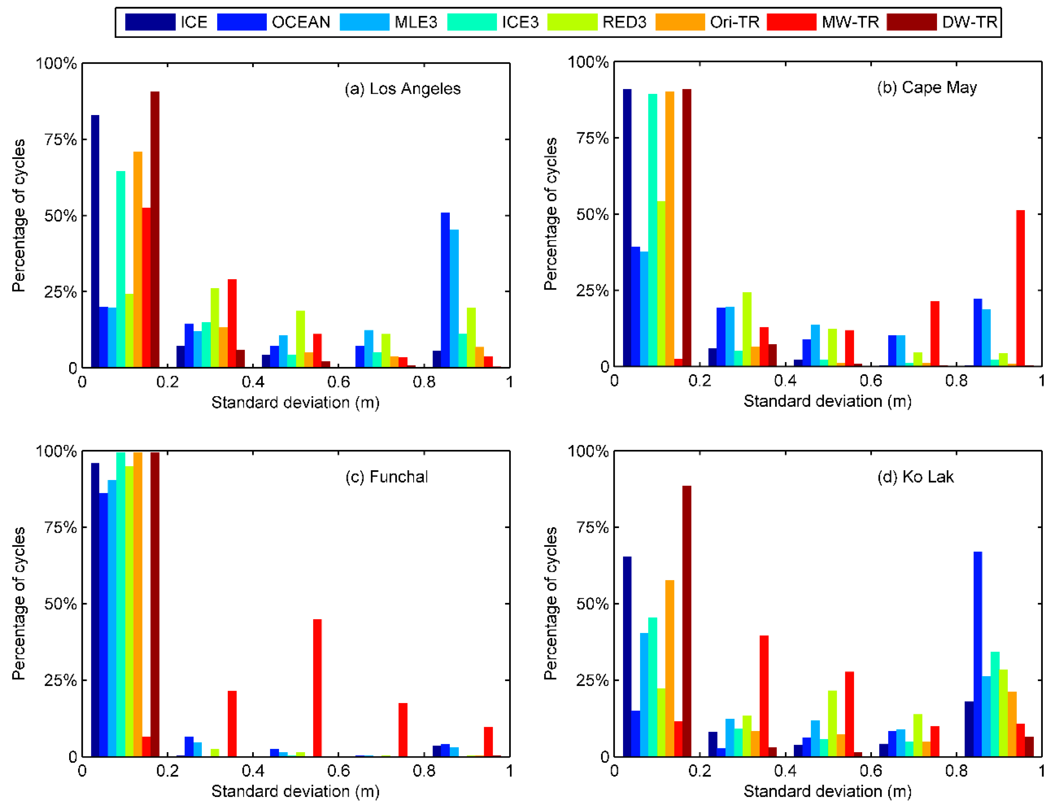
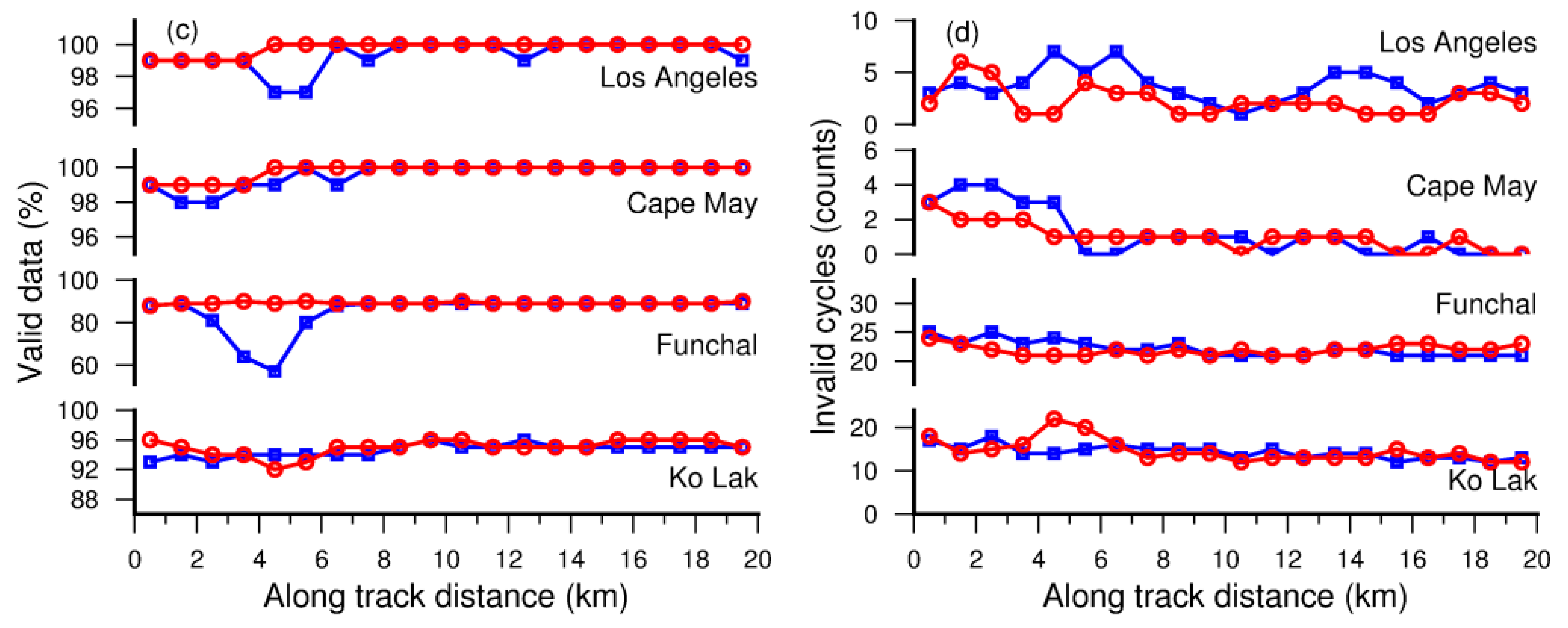
The SDs of the difference between various retracked along-track SSHs and geoid within 10 km away from the coastline are computed for all cycles after discarding crude measurements by a 3σ de-outlier process. Figure 4 shows histograms of the SDs in the four study regions. Table 3 presents the mean SDs before and after removing outliered cycles (>3σ) and corresponding improvement percentage (IMP) [32] relative to the non-retracked SSHs. The SD after removing outliered cycles is denoted as Cal. SD in Table 3 and the following table. The highest precision and the maximum IMPs are indicated by underlined numbers. The percentages of valid data and numbers of invalid cycles are also tabulated in Table 3.
It is notable that DW-TR exhibits better performance than the other retrackers. In overall average, DW-TR preserves most of data points (97%) and achieves the largest improvement, which is about 82% and 89% before and after the calibration, respectively. It exceeds two 30% threshold retrackers, ICE and ICE3, by 5% and 15% in accuracy, respectively. For the same 20% threshold retrackers, DW-TR outperforms Ori-TR by 9% and MW-TR by 34%. It indicates that the waveform decontamination procedure can efficiently reduce the superimposed noise in coastal waveforms. Overall, three model-based retrackers (OCEAN, MLE3 and RED3) have more data loss and less improvement in accuracy than threshold retrackers. In region (a), OCEAN and MLE3 retracked results are even worse than the non-retracked SSHs. Obviously, the redundant peaks in waveforms will cause the fitted waveform using the Brown model to deviate seriously from the actual waveform. Although RED3 applies a window to filter the waveform, its improvement is not significant.
Histograms in Figure 4 also illustrate that DW-TR is the most robust retracker. For the DW-TR retracked SSHs, more than 85% of cycles have the SD <0.2 m in all the four cases. The OCEAN retracker is less robust compared to the other retrackers. It can be found over region (a) and (d) that the precision of OCEAN retracked measurements is larger than 0.8 m for more than 50% of cycles. Furthermore, frequency of high precision (<0.2 m) cycles for MW-TR is relatively less than the other retrackers. It is particularly evident in region (b). This result indicates that the precision of MW-TR retracked measurements in many cycles deteriorate after waveform modification.
4.2. Comparison to Tide Gauge Data
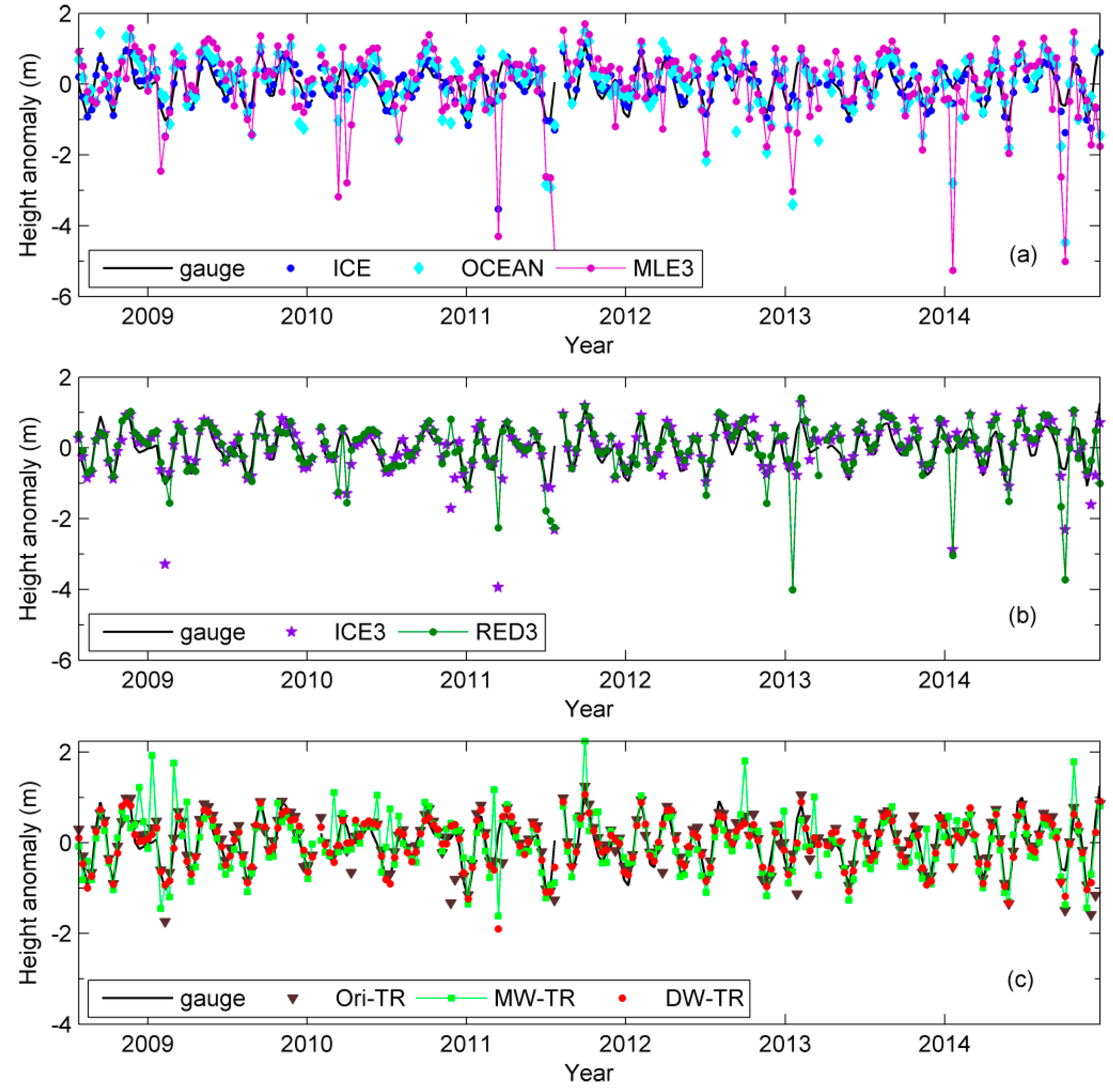
Figure 5 shows an example of coastal (0–10 km) SSH variation from each retrackers in region (a). Temporal mean is subtracted from each time series, referring to as height anomaly. It is obvious that the measurements from SGDR and PISTACH products are much noisy than those of DW-TR with respect to tide gauge. In Figure 5a, the OCEAN and MLE3 retracked SSHs are apparently more dispersed than the ICE results. Figure 5b illustrates that the SSHs from ICE3 and RED3 in many cycles are largely deviated from the gauge data. Figure 5c presents the results from three 20% threshold retrackers using original, modified and decontaminated waveforms, respectively. The retracked results by DW-TR are most consistent with the gauge data. It is evident that a number of deviated cycles exist in the time series estimated by MW-TR.
The statistical results of comparison over the four study regions are summarized in Table 4. The results show, on average, DW-TR yields the smallest SDs and the highest IMPs. It also obtains the largest number of valid data and the smallest number of invalid cycles. Furthermore, DW-TR presents the highest correlation between height anomaly and tide gauge. It is the only retracker with a mean correlation coefficient higher than 0.9. Compared to Ori-TR, DW-TR achieves 40% (50–30 cm) improvement before calibration and 33% (30–20 cm) after calibration, whilst a decrease in accuracy from MW-TR is observed. MW-TR is better than Ori-TR only in region (d). Concerning retrackers in SGDR and PISTACH products, ICE performs with greater stability than the other retrackers. In some cases (e.g., near Cape May coast), ICE provides comparable results to DW-TR. Negative IMPs appear in some cases for OCEAN, MLE3, ICE3 and RED3, indicating that these retrackers are unreliable. Although the PISTACH retrackers are developed for coastal applications, their performance should be evaluated case by case. For instance, the results of ICE3 are better in region (c), but worse in the other regions than those of the ICE retracker.
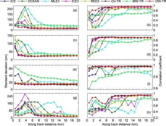
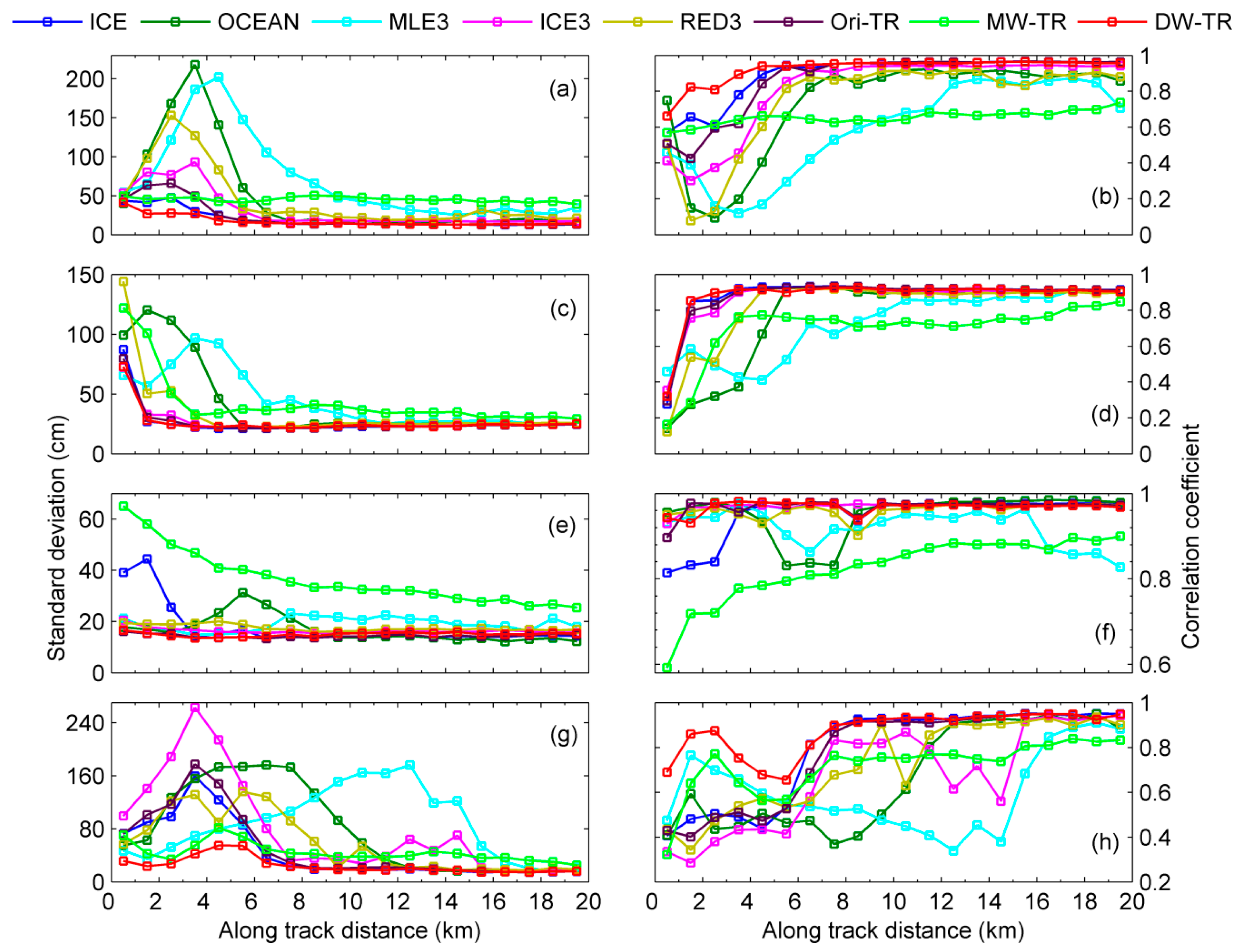
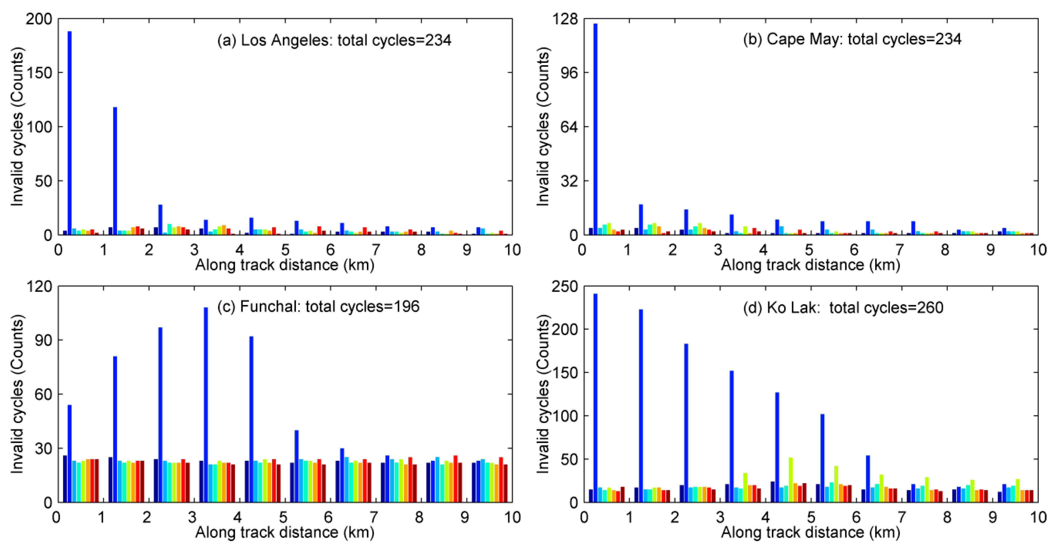
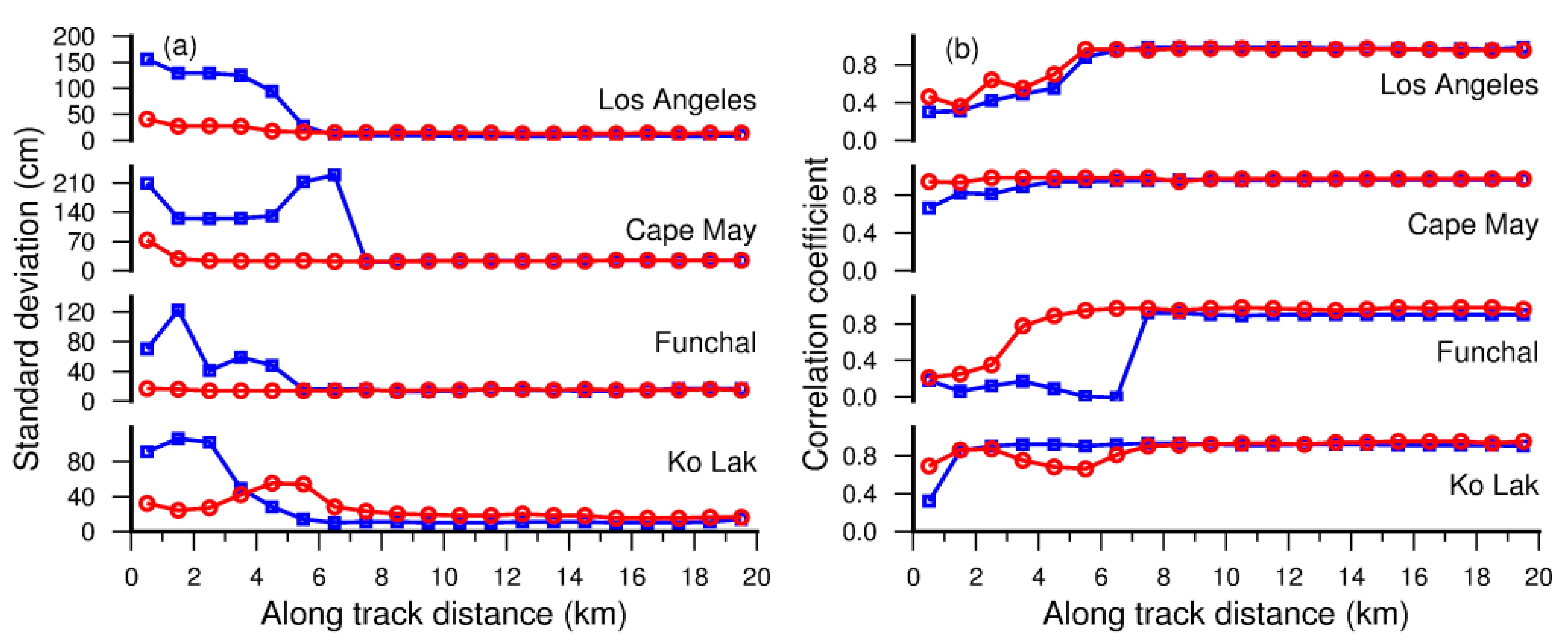
In order to assess how close each retracker can extend precise measurements to the coastline, the SDs and correlation coefficients over each 1-km band within 20 km of the shoreline are computed, which are shown in Figure 6 in terms of along-track distance. It can be seen that DW-TR achieves the smallest SDs and the highest correlation in all cases within 10 km of the shoreline, whilst performing as well as OCEAN, ICE, and Ori-TR in the 10–20 km zone. It can extend measurements to 1 km offshore with nearly consistent accuracy and data gaps as well as high correlation, except for in region (d). There is a peninsula extruding toward the middle segment of the selected satellite track in region (d), which results in large error and low correlation at an along-track distance of 4–6 km. As expected, the performance of OCEAN gets worse when approaching the coast. Data gaps in each band within 10 km for different retrackers are illustrated in Figure 7. From 7 km, the number of invalid cycles for OCEAN is significantly larger than those of other retrackers. Although the OCEAN retracker achieves high accuracy in area very near close to the coast sometimes, it is based on very huge data gaps as displayed in Figure 7.
5. Discussion
5.1. Negative Effects of Contaminations in Coastal Waveforms on Retrackers
Comparison results in Section 4 demonstrate the inefficiency of Brown-model-based retrackers (OCEAN, MLE3, RED3 and OCE3) for coastal altimetry. Obviously, the estimates from the maximum likelihood estimator applied to the Brown model cannot accurately reproduce the variations of the coastal waveform, due to the superimposed echoes from non-marine surfaces [6]. On the other hand, the contamination in coastal waveform may disturb the estimation of waveform amplitude, and then lead to unreliable retracked SSHs from empirical retrackers [43]. In general, SSHs will be underestimated by OCOG and threshold retrackers due to the anomalous peaks. It can explain why the empirical retrackers (ICE, ICE3 and Ori-TR) using original waveforms have inconsistent accuracy along the distance to the coast (see Figure 6), and have a relatively large number of invalid cycles (see Table 3 and Table 4).
The subwaveform technique may improve the precision of altimeter observations. But it is difficult to accurately extract the subwaveform, when there are multiple peaks or an excessive peak in the waveform. Anomalous peaks may mislead the judgment of the leading edge, thus resulting in seriously deviated height estimations. This is the reason that the ICE3 and RED3 retrackers, which retrack portion samples of the waveform, show worse performance and less valid data in some cases. To further discuss the performance of subwaveform retrackers in coastal area, we analyzed the state-of-the-art ALES (Adaptive Leading Edge Subwaveform) product in the four study regions. ALES picks out subwaveform including the leading edge using an adaptive window, and models it with the classic Brown model by means of least square estimation [38]. According to the result in Figure 8, ALES works effectively to about 8 km offshore. The best case is near Ko Lak, Thailand, where SSHs from ALES have much higher accuracy than those from DW-TR up to 4 km offshore. However, the ALES outputs show significant degradation over areas very close to land. The same result was found around the Tsushima Island in Japan [54]. Apparently, ALES does not completely overcome the difficult problem of accurate subwaveform extraction in coastal ocean.
5.2. Improvement of the WD with Respect to the WM
In nature, the effect of the WM and the WD is not to improve the retracking algorithm, but to purify waveforms. It is similar to the subwaveform technique to some extent. The subwaveform approach excludes polluted samples by selecting part of each waveform, while the modification procedure is designed to detect and remedy spurious samples by some empirical methods.
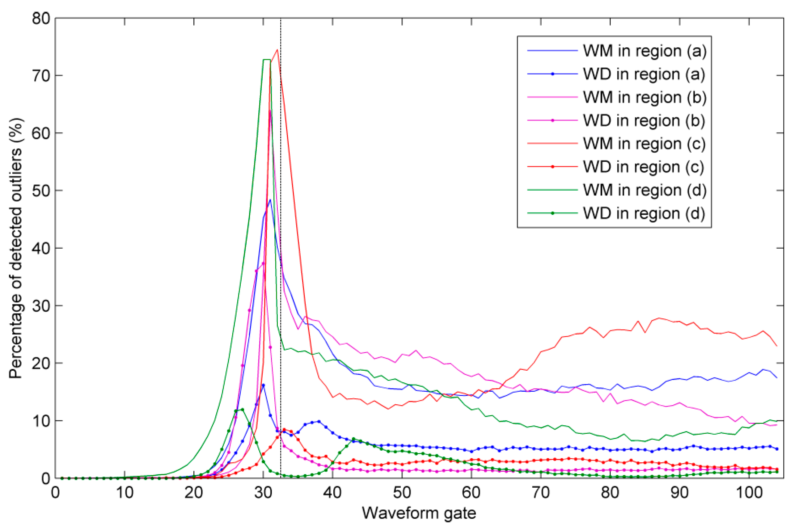
As pointed out in Section 3.1, shifts of the leading edges of the waveforms will cause the failure of the WM procedure. In ocean-land or land-ocean transition zones, these shifts will be frequently introduced by the tracker algorithm, which is based on the determination of the center of gravity of the waveform energy [55]. Most of sampling gates in the shifted leading edges will be misjudged as outliers by the WM method (see Figure 9). Therefore, retracking modified waveforms does not achieve similar average accuracy compared to retracking original waveforms over the four test regions. From Figure 9, it can be seen that outliers detected by the WD are much less than those by the WM. The WD method presented in this paper successfully overcomes the insufficiency of WM. All results validate the highest performance of the DW-TR retracker which is based on purified waveforms by the WD.
5.3. Bias Analysis
Biases between DW-TR, Ori-TR and OCEAN retrackers were estimated for each region, presented in Table 5. Biases were computed by averaging differences between two retracked SSH sets within 13–20 km where correlation coefficients were higher than 0.9 for the three retrackers and for the four considered regions. Biases of DW-TR and Ori-TR relative to OCEAN are of the same order of 65 to 78 cm, with standard deviation of the order of 6 to 11 cm. Biases between DW-TR and Ori-TR are of the order of 1 cm with standard deviation less than 2 cm. It implies that the WD method proposed in this paper will not induce a significant bias into the SSH estimations. The bias between DW-TR and OCEAN is mainly a result of the difference between the 20% threshold retracker and the OCEAN retracker. Therefore, for operational applications covering a larger area, the WD method can still improve the accuracy of SSHs without significant biases, if the same retracker is employed for retracking decontaminated waveforms in coastal regions and original waveforms in open oceans.
5.4. Test for Tracks Paralleling or Crossing Intricate Coastlines
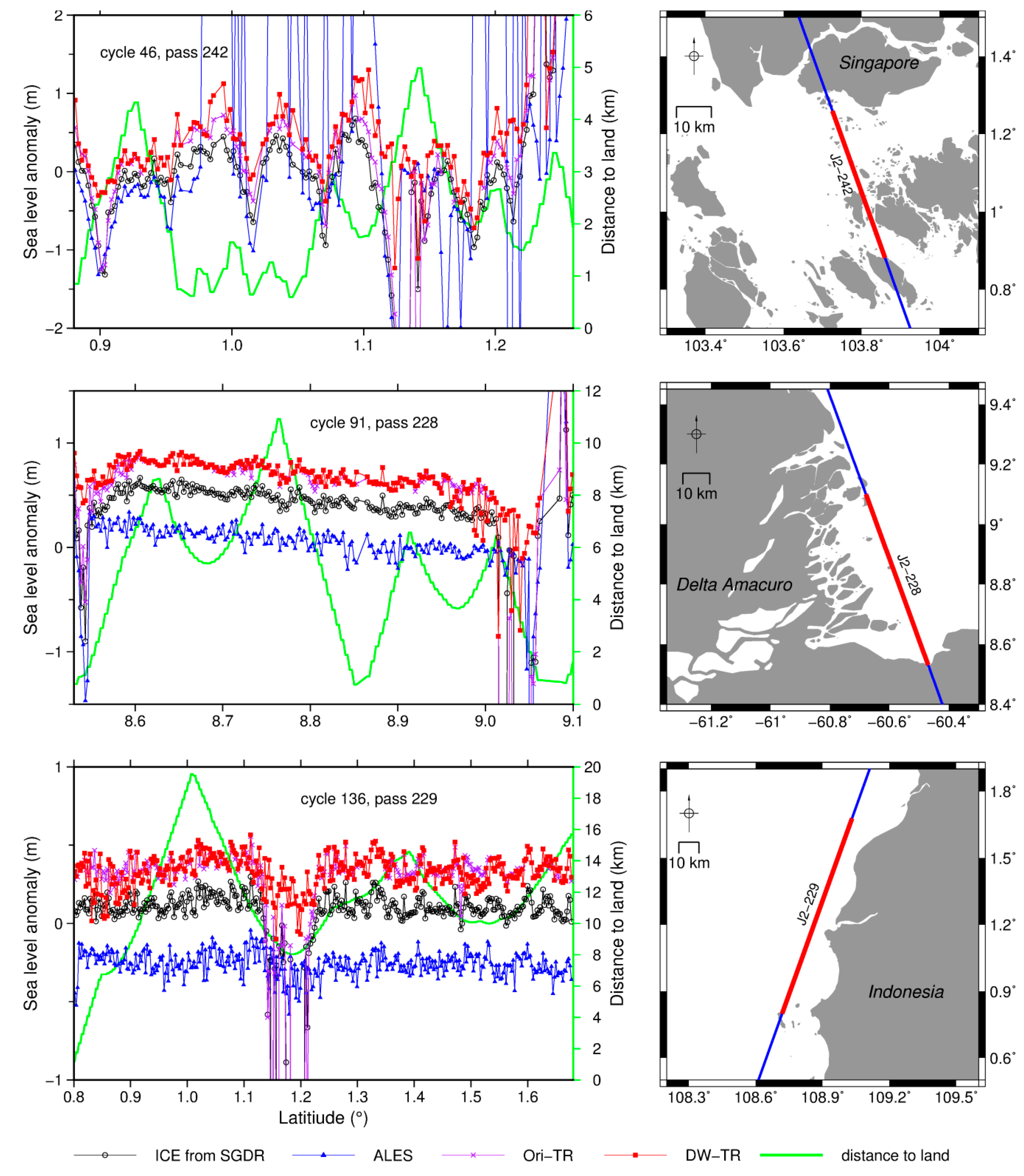
To test the ability of our proposed method in more complicated situations, experiments were performed for three more tracks passing through areas with different types of coastlines. The first track with a length of about 100 km is taken from pass 229, which is nearly parallel to the northwest coast of Indonesia (the bottom in Figure 10). There is an island in the south end of this track. Maximum distance to land is less than 20 km. The second track from pass 228 is located near the Delta Amacuro in Venezuela (the middle in Figure 10). A 65 km long segment is truncated in which the longest distance to land is about 11 km. Many small islands distribute on the side of the track where the river estuary is. The third one is a 45-km-long track from pass 242, located in the Singapore Strait. There are lots of islands on both sides of the track. The farthest distance away from land is less than 5 km, and then almost every waveform on this track contains land contamination.
Since tide gauge data are not available, we compared the sea level anomaly (SLA) from DW-TR to those from ICE, ALES and Ori-TR retrackers. Figure 10 shows examples of SLA profiles from different retrackers. For all cases, reference waveform used in the WD was averaged using all waveforms in the selected track. It can be seen that DW-TR shows robust performance in three cases. For pass 229, the performance of ALES and DW-TR is better than those of ICE and Ori-TR retrackers. ICE and Ori-TR suffer from large errors in the region close to the tongue at a latitude of about 1.2°. Obviously, anomalous peaks cause the sea level to be underestimated by ICE and Ori-TR. The subwaveform technique and the WD process can exclude or remove anomalous peaks well in this case. For pass 228, four retrackers work well except at both ends of the track where the satellite nadirs are much closer to coastline. Compared to other retrackers, the DW-TR obtains a relatively larger number of reasonable SLAs where the distance to land is less than 5 km. In the case of pass 242, the performance of ICE, Ori-TR and ALES becomes worse, while the DW-TR still keeps high effectivity and reliability. Comparisons of SLAs by the DW-TR with those by the Ori-TR further confirm that the WD may not produce a significant bias.
5.5. Issues for Further Research
Although the WD method was validated in several regions in this study, more validations are needed for future global coastal applications since coastal situations are so complicated and quite different everywhere. It is worth mentioning the important role of the reference waveform for the WD. The impact of the reference waveform and it optimal determination might be worthy of further study. No strict rule for the selection of the reference waveform is given in this study. But it should be kept in mind that the reference waveform has to contain information of coastal waveforms to be modified.
It is difficult to accurately detect all contaminated samples in a waveform in a simple way. Underestimation of SLA at both ends of track 228 in Figure 10 implies that there are still some anomalous peaks remained after the WD. Therefore, there is certainly room for improvement of outlier detection. Realigning along-track waveforms [39,54] before the WD might be a good way to further improve outlier detection, which is under investigation.
It should be emphasized that we used the same SSB corrections for all the retracked SSHs, which might induce some errors. The SSB is the sum of electromagnetic bias, skewness bias and tracker bias [25,45]. The accuracy of the SSB is mainly up to the accuracy of estimated significant wave height (SWH), varying with different retrackers. It is expected that the retracked SSHs can be further improved by applying SSB correction corresponding to the specific retracker. Focusing on the performance of various retrackers, SWH is not estimated in this study. It remains a topic of research to assess the impact of SSB on the retracked results.
6. Conclusions and Recommendations
It is proved that removing the superimposed signals from non-marine surfaces by empirical or model-fitting methods is helpful to improve the performance of waveform retracking [6,39,43]. In this paper, an improved empirical method for waveform decontamination was developed based on the WM algorithm. According to the experiments over four coastal regions with different situations, retracked SSHs using the decontaminated waveforms are superior to those using original waveforms and modified waveforms. Comparison results also suggest the DW-TR retracker outperforms SGDR, PISTACH and ALES retrackers in terms of accuracy and data coverage within 10 km offshore. It should be emphasized that the WD method is appropriate for other altimeter data, although it was only validated here using Jason-2 altimeter data. Moreover, only the 20% threshold retracker was applied on the decontaminated waveforms as SSHs were concerned in the present study. In order to extract more parameters, such as significant wave height, model-based retrackers should be used. Theoretically, all retrackers can be exploited to retrack the decontaminated waveforms. Their performance, however, should be further evaluated.
For the SGDR products, ICE provides more accurate measurements than OCEAN and MLE3 in coastal areas, which is consistent with previous studies [33,43]. It is reasonable since in some degree, the ICE retracker moderates the influence of excessive energy in the trailing edge by combining threshold and OCOG retrackers. The performance of ICE3 and RED3 in PISTACH products is not stable. Generally speaking, the two retrackers have high accuracy beyond about 8 km offshore, and become worse in the 0–8 km coastal band. The same performance can be found for ALES in the four study regions. It indicates that these subwaveform retrackers encounter a barrier to accurately extract noise-free subwaveforms in coastal oceans very close to land.
The main purpose of this study is to improve SSHs within 10 km offshore. Experiments in the four study regions were performed using data in the 0–20 km coastal band. The subsequent test in three particular cases shows the new retracking strategy based on the WD proposed here is not limited to a 20 km wide strip along the coast, and can adapt to diverse complicated situations. So, it has great potential for operational application in the global coastal zone. Another advantage of the WD method is that it will not induce a bias between coastal regions and open oceans, as long as the same retracker is applied on decontaminated waveforms and original waveforms. This feature may extend applications of the new method to a larger area. With the help of the WD, the retracking process can achieve more accurate coastal altimetry data with the ability to compare them to the data from open oceans. It will greatly benefit coastal applications connected to sea level, such as coastal circulation studies, coastal tide modelling and refining gravity field in coastal zones. By combining the WD with sophisticated retrackers, significant wave height and backscatter coefficient are expected to be acquired with a higher accuracy, which is helpful for monitoring coastal sea state. This work will be performed in the future study.
Acknowledgments
We acknowledge AVISO for the Jason-2 SGDR data, CLS for the PISTACH data, and UHSLC for the tide gauge data used in this study. The ALES data were obtained from JPL Physical Oceanography DAAC and developed by the UK National Oceanography Centre. This work was supported by the National Natural Science Foundation of China (Grant No. 41774010, 41174021, 41429401), by the Open Fund of Guangxi Key Laboratory of Spatial Information and Geomatics (Grant No. 15-140-07-26), and by the Belmont Forum/IGFA G8 Coastal Vulnerability Program via the United States National Science Foundation (Grant No. CER-1342644).
Author Contributions
Haihong Wang and Zhicai Luo conceived and designed the experiments; Zhengkai Huang and Haihong Wang performed the experiments and wrote the first draft; all authors analyzed the data and wrote the final draft.
Conflicts of Interest
The authors declare no conflict of interest. The founding sponsors had no role in the design of the study; in the collection, analyses, or interpretation of data; in the writing of the manuscript, and in the decision to publish the results.
References
- Fu, L.L.; Cazenave, A. Satellite Altimetry and Earth Sciences: A Handbook of Techniques and Applications; Academic Press: San Diego, CA, USA, 2001. [Google Scholar]
- Deng, X.; Featherstone, W.E.; Hwang, C.; Berry, P.A.M. Estimation of contamination of ERS-2 and POSEIDON satellite radar altimetry close to the coast of Australia. Mar. Geodesy 2002, 25, 249–271. [Google Scholar] [CrossRef]
- Vignudelli, S.; Cipollini, P.; Roblou, L.; Lyard, F.; Gasparini, G.P.; Manzella, G.; Astraldi, M. Improved satellite altimetry in coastal systems: Case study of the Corsica Channel (Mediterranean Sea). Geophys. Res. Lett. 2005, 32, L07608. [Google Scholar] [CrossRef]
- Gómez-Enri, J.; Cipollini, P.; Passaro, M.; Vignudelli, S.; Tejedor, B.; Coca, J. Coastal altimetry products in the Strait of Gibralta. IEEE Trans. Geosci. Remote Sens. 2016, 54, 5455–5466. [Google Scholar] [CrossRef]
- Deng, X. Improvement of Geodetic Parameter Estimation in Coastal Regions from Satellite Radar Altimetry. Ph.D. Thesis, Curtin University of Technology, Perth, Australia, 2004. [Google Scholar]
- Halimi, A.; Mailhes, C.; Tourneret, J.Y.; Thibaut, P.; Boy, F. Parameter estimation for peaky altimetric waveforms. IEEE Trans. Geosci. Remote Sens. 2013, 51, 1568–1577. [Google Scholar] [CrossRef] [Green Version]
- Anderson, O.B.; Scharroo, R. Range and geophysical corrections in coastal regions: And implications for mean sea surface determination. In Coastal Altimetry; Vignudelli, S., Kostianoy, A.G., Cipollini, P., Benveniste, J., Eds.; Springer: Berlin, Germany, 2011; pp. 103–145. [Google Scholar]
- Feng, H.; Vandemark, D. Altimeter data evaluation in the coastal gulf of Maine and Mid-Atlantic bight regions. Mar. Geodesy 2011, 34, 340–363. [Google Scholar] [CrossRef]
- Idris, N.H.; Deng, X.L.; Anderson, O.B. The importance of coastal altimetry retracking and detiding: A case study around the Great Barrier Reef, Australia. Int. J. Remote Sens. 2014, 35, 1729–1740. [Google Scholar] [CrossRef]
- Vignudelli, S.; Snaith, H.M.; Lyard, F.; Cipollini, P.; Venuti, F.; Birol, F.; Bouffard, J.; Roblou, L. Satellite radar altimetry from open ocean to coasts: Challenges and perspectives. In Proceedings of the 5th Asia-Pacific Remote Sensing Symposium, Goa, India, 13–17 November 2006; Volume 6406, pp. 1–12. [Google Scholar]
- Reale, F.; Dentale, F.; Pugliese Carratelli, E.; Torrisi, L. Remote sensing of small-scale storm variations in coastal seas. J. Coast. Res. 2014, 30, 130–141. [Google Scholar] [CrossRef]
- Vincent, P.; Steunou, N.; Caubet, E.; Phalippou, L.; Rey, L.; Thouvenot, E.; Verron, J.; AltiKa, A. Ka-band altimetry payload and system for operational altimetry during the GMES period. Sensors 2006, 6, 208–234. [Google Scholar] [CrossRef]
- Raney, R.K. The delay/Doppler radar altimeter. IEEE Trans. Geosci. Remote Sens. 1998, 36, 1578–1588. [Google Scholar] [CrossRef]
- Halimi, A.; Mailhes, C.; Tourneret, J.Y.; Boy, F.; Moreau, T. Including antenna mispointing in a semi-analytical model for delay/Doppler altimetry. IEEE Trans. Geosci. Remote Sens. 2015, 53, 598–608. [Google Scholar] [CrossRef]
- Lowe, S.T.; Zuffada, C.; Chao, Y.; Kroger, P.; Young, L.E.; LaBrecque, J.L. 5-cm-precision aircraft ocean altimetry using GPS reflections. Geophys. Res. Lett. 2002, 29, 131–134. [Google Scholar] [CrossRef]
- Allan, T. The story of GANDER. Sensors 2006, 6, 249–259. [Google Scholar] [CrossRef]
- Enjolras, V.; Vincent, P.; Souyris, J.C.; Rodriguez, E.; Phalippou, L.; Cazenave, A. Performances study of interferometric radar altimeters: From the instrument to the global mission definition. Sensors 2006, 6, 164–192. [Google Scholar] [CrossRef]
- Anzenhofer, M.; Shum, C.K.; Rentsh, M. Coastal Altimetry and Applications; Report No. 464; Geodetic Science and Surveying, The Ohio State University: Columbus, OH, USA, 1999. [Google Scholar]
- Bouffard, J.; Vignudelli, S.; Cipollini, P.; Menard, Y. Exploiting the potential of an improved multimission altimetric data set over the coastal ocean. Geophys. Res. Lett. 2008, 35, L10601. [Google Scholar] [CrossRef]
- Cipollini, P.; Calafat, F.M.; Jevrejeva, S.; Melet, A.; Prandi, P. Monitoring sea level in the coastal zone with satellite altimetry and tide gauges. Surv. Geophys. 2016, 38, 33–57. [Google Scholar] [CrossRef]
- Mercier, F.; Rosmorduc, V.; Carrere, L.; Thibaut, P. Coastal and Hydrology Altimetry Product (PISTACH) Handbook. CLS-DOS-NT-10-246, SALP-MU-P-OP-16031-CN 01/00. 2010. Available online: https://www.aviso.altimetry.fr/fileadmin/documents/data/tools/hdbk_Pistach.pdf (accessed on 23 October 2017).
- Cipollini, P.; Susana Barbosa, S.; Caparrini, M.; Challenor, P.; Coelho, H.; Dinardo, S.; Fernandes, S.; Gleason, S.; Gómez-Enri, J.; Gommenginger, C.; et al. COASTALT Project’s contribution to the development and dissemination of coastal altimetry. In Proceedings of the 20 Years of Progress in Radar Altimetry Symposium, Venice, Italy, 24–29 September 2012. [Google Scholar]
- Birol, F.; Fuller, N.; Lyard, F.; Cancet, M.; Nino, F.; Delebecque, C.; Léger, F. Coastal applications from nadir altimetry: Example of the X-TRACK regional products. Adv. Space Res. 2017, 59, 936–953. [Google Scholar] [CrossRef]
- Vignudelli, S.; Kostianoy, A.G.; Cipollini, P.; Benveniste, J. Coastal Altimetry; Springer: Berlin, Germany, 2011. [Google Scholar]
- Tran, N.; Vandemark, D.; Chapron, B.; Labroue, S.; Feng, H.; Beckley, B.; Vincent, P. New models for satellite altimeter sea state bias correction developed using global wave model data. J. Geophys. Res. 2006, 111, C09009. [Google Scholar] [CrossRef]
- Feng, H.; Yao, S.; Li, L.; Tran, N.; Vandemark, D.; Labroue, S. Spline-based nonparametric estimation of the altimeter sea-state bias correction. IEEE Geosci. Remote Sens. Lett. 2010, 7, 577–581. [Google Scholar] [CrossRef]
- Tran, N.; Vandemark, D.; Labroue, S.; Feng, H.; Chapron, B.; Tolman, H.L.; Lambin, J.; Picot, N. Sea state bias in altimeter sea level estimates determined by combining wave model and satellite data. J. Geophys. Res. 2010, 115, C03020. [Google Scholar] [CrossRef]
- Pires, N.; Fernandes, M.; Gommenginger, C.; Scharroo, R. A Conceptually Simple Modeling Approach for Jason-1 Sea State Bias Correction Based on 3 Parameters Exclusively Derived from Altimetric Information. Remote Sens. 2016, 8, 576. [Google Scholar] [CrossRef]
- Reale, F.; Dentale, F.; Pugliese Carratelli, E. Numerical simulation of whitecaps and foam effects on satellite altimeter response. Remote Sens. 2014, 6, 3681–3692. [Google Scholar] [CrossRef]
- Brown, G. The average impulse response of a rough surface and its applications. IEEE Trans. Antennas Propag. 1977, 25, 67–74. [Google Scholar] [CrossRef]
- Davis, C.H. A robust threshold retracking algorithm for measuring ice-sheet surface elevation change from satellite radar altimeters. IEEE Trans. Geosci. Remote Sens. 1997, 35, 974–979. [Google Scholar] [CrossRef]
- Hwang, C.; Guo, J.Y.; Deng, X.L.; Hsu, H.Y.; Liu, Y.T. Coastal gravity anomalies from retracked Geosat/GM altimetry: Improvement, limitation and the role of airborne gravity data. J. Geodesy 2006, 80, 204–216. [Google Scholar] [CrossRef]
- Lee, H.; Shum, C.K.; Emery, W.; Calmant, S.; Deng, X.; Kuo, C.Y.; Roesler, C.; Yi, Y.C. Validation of Jason-2 altimeter data by waveform retracking over California coastal ocean. Mar. Geodesy 2010, 33, 304–316. [Google Scholar] [CrossRef]
- Guo, J.; Gao, Y.; Hwang, C.; Sun, J. A mutli-subwaveform parametric retracker of the radar satellite altimetric waveform and recovery of gravity anomalies over coastal oceans. Sci. China Earth Sci. 2010, 53, 610–616. [Google Scholar] [CrossRef]
- Yang, Y.; Hwang, C.; Hsu, H.J.; Dongchen, E.; Wang, H. A subwaveform threshold retracker for ERS-1 altimetry: A case study in the Antarctic Ocean. Comp. Geosci. 2012, 41, 88–98. [Google Scholar] [CrossRef]
- Yang, L.; Lin, M.; Liu, Q.; Pan, D. A coastal altimetry retracking strategy based on waveform classification and subwaveform extraction. Int. J. Remote Sens. 2012, 33, 7806–7819. [Google Scholar] [CrossRef]
- Idris, N.H.; Deng, X. The retracking technique on multi-peak and quasi-specular waveforms for Jason-1 and Jason-2 missions near the coast. Mar. Geodesy 2012, 35, 217–237. [Google Scholar] [CrossRef]
- Passaro, M.; Cipollini, P.; Vignudelli, S.; Quartly, G.D.; Snaith, H.M. ALES: A multi-mission adaptive subwaveform retracker for coastal and open sea altimetry. Remote Sens. Environ. 2014, 145, 173–189. [Google Scholar] [CrossRef] [Green Version]
- Gómez-Enri, J.; Vignudelli, S.; Quartly, G.D.; Gommenginger, C.P.; Cipollini, P.; Challenor, P.G.; Benveniste, J. Modeling ENVISAT RA-2 waveforms in the coastal zone: Case study of calm water contamination. IEEE Geosci. Remote Sens. Lett. 2010, 7, 474–478. [Google Scholar] [CrossRef] [Green Version]
- Deng, X.; Featherstone, W. A coastal retracking system for satellite radar altimeter waveforms: Application to ERS-2 around Australia. J. Geophys. Res. 2006, 111, C06012. [Google Scholar] [CrossRef]
- Wang, H.H.; Luo, Z.C.; Yang, Y.D.; Zhong, B.; Zhou, H. An adaptive retracking method for coastal altimeter data based on waveform classification. Acta Geodesy Cartogr. Sin. 2012, 41, 729–734. [Google Scholar]
- Khakia, M.; Forootan, E.; Sharifi, M.A. Satellite radar altimetry waveform retracking over the Caspian Sea. Int. J. Remote Sens. 2014, 35, 6329–6356. [Google Scholar] [CrossRef]
- Tseng, K.H.; Shum, C.K.; Yi, Y.C.; Emery, W.J.; Kuo, C.Y.; Wang, H.H. The improved retrieval of coastal sea surface heights by retracking modified radar altimetry waveforms. IEEE Trans. Geosci. Remote Sens. 2014, 52, 991–1001. [Google Scholar] [CrossRef]
- Desjonquères, J.D.; Carayon, G.; Steunou, N.; Lambin, J. Poseidon-3 radar altimeter: New modes and in-flight performances. Mar. Geodesy 2010, 33, 53–79. [Google Scholar] [CrossRef]
- AVISO+ CNES. Available online: https://www.aviso.altimetry.fr/en/missions/current-missions/jason-2/index.html (accessed on 20 May 2017).
- Lambin, L.; Morrow, R.; Fu, L.L.; Willis, J.; Bonekamp, H.; Lillibridge, J.; Perbos, J.; Zaouche, G.; Vaze, P.; Bannoura, W.; et al. The OSTM/Jason-2 mission. Mar. Geodesy 2010, 33, 4–25. [Google Scholar] [CrossRef]
- Chelton, D.B.; Ries, J.C.; Haines, B.J.; Fu, L.-L.; Callahan, P.S. Satellite Altimetry. In Satellite Altimetry and Earth Sciences: A Handbook of Techniques and Applications; Fu, L.-L., Cazenave, A., Eds.; Academic Press: San Diego, CA, USA, 2001; pp. 1–131. [Google Scholar]
- Dumont, J.-P.; Rosmordue, V.; Picot, N.; Desai, S.; Bonekamp, H.; Figa, J.; Lillibridge, J.; Sharroo, R. OSTM/Jason-2 Products Handbook. CNES: SALP-MU-M-OP-15818-CN; EUMETSAT: EUM/OPS-JAS/MAN/08/0041; JPL: OSTM-29–1237; NOAA/NESDIS: Polar Series/OSTM J400; 2011; Available online: https://www.aviso.altimetry.fr/fileadmin/documents/data/tools/hdbk_j2.pdf (accessed on 23 October 2017).
- Wingham, D.J.; Rapley, C.G.; Griffiths, H. New techniques in satellite altimeter tracking systems. In Proceedings of the 1986 International Geoscience and Remote Sensing Symposium on Remote Sensing: Today’s Solutions for Tomorrow’s Information Needs, Noordwijk, The Netherlands, 8– 11September 1986; Volume 3, pp. 1339–1344. [Google Scholar]
- Gommenginger, C.; Thibaut, P.; Fenoglio-Marc, L.; Quartly, G.; Deng, X.; Gómez-Enri, J.; Challenor, P.; Gao, Y. Retracking altimeter waveforms near the coasts. In Coastal Altimetry; Vignudelli, S., Kostianoy, A.G., Cipollini, P., Benveniste, J., Eds.; Springer: Berlin, Heidelberg, 2011; pp. 61–102. [Google Scholar]
- Becker, J.J.; Sandwell, D.T.; Smith, W.H.F.; Braud, J.; Binder, B.; Depner, J.; Fabre, D.; Factor, J.; Ingalls, S.; Kim, S.H.; et al. Global bathymetry and elevation data at 30 arc seconds resolution: SRTM30_PLUS. Mar. Geodesy 2009, 32, 355–371. [Google Scholar] [CrossRef]
- Caldwell, P.C.; Merrfield, M.A.; Thompson, P.R. Sea Level Measured by Tide Gauges from Global Oceans—The Joint Archive for Sea Level Holdings (NCEI Accession 0019568), Version 5.5. NOAA National Centers for Environmental Information, Dataset. 2015. Available online: https://uhslc.soest.hawaii.edu/datainfo/ (accessed on 23 October 2017).
- Pavlis, N.K.; Holmes, S.A.; Kenyon, S.C.; Factor, J.K. The development and evaluation of the Earth Gravitational Model 2008 (EGM2008). J. Geophys. Res. 2012, 117, B04406. [Google Scholar] [CrossRef]
- Wang, X.; Ichikawa, K. Coastal waveform retracking for Jason-2 altimeter data based on along-track echograms around the Tsushima Islands in Japan. Remote Sens. 2017, 9, 762. [Google Scholar] [CrossRef]
- Thibaut, P.; Poisson, J.C.; Bronner, E.; Picot, N. Relative performance of the MLE3 and MLE4 retracking algorithms on Jason-2 altimeter waveforms. Mar. Geodesy 2010, 33, 317–335. [Google Scholar] [CrossRef]
Figure 1.
Study regions: (a) Los Angeles, CA, USA; (b) Cape May, NJ, USA; (c) Funchal, Madeira Island, Portugal; (d) Ko Lak, Prachuap Khiri Khan, Thailand. Red line denotes ground track of Jason-2 satellite. Orientation of the pass tag over the red line implies flight direction of the satellite. Evaluated data are located within the rectangle with the white dashed line. Gauge station is marked as the white pentacle with black edge. Topography is extracted from the digital elevation model SRTM30-plus [51]. Interpolated along-track ocean depth within 0–10 km offshore is plotted in the sub-panel.

Figure 2.
Failed case of coastal waveform modification illustrated by Jason-2 pass #228, cycle #50, near Cape May, NJ, USA. White dashed line shows the nominal tracking gate. The upper boundary in latitude indicates the coastline. Waveforms along with latitude are color-coded by waveform sampling power. (a) Original waveforms; (b) Absolute residual waveforms relative to the mean waveform over 20–30 km offshore; (c) Modified waveforms.

Figure 3.
Comparison between waveform modification (WM) and waveform decontamination (WD) in the case of Figure 2. Reference waveforms for the two methods are shown in (a). The blue one is used in the WM, averaged within 20–30 km offshore. The red one is used in the WD, averaged between 0–20 km offshore. The black curve with dots is the observed waveform at latitude 38.84°. Its corresponding residual waveforms are shown in (b). The blue circles and the red triangles denote anomalous samples detected by WM and WD, respectively.

Figure 4.
Histograms for standard deviations of various retracked sea surface heights (SSHs) relative to geoid in four study regions: (a) Los Angeles, (b) Cape May, (c) Funchal, (d) Ko Lak. All available cycles are included for statistical analysis. Only frequencies of standard deviations less than 1 m are plotted with the step of 0.2 m. Retrackers are represented by different colors shown in the upmost legend.

Figure 5.
Coastal (0–10 km) SSH variation from different retrackers: (a) Sensor geophysical data record (SGDR) retrackers; (b) Prototype Innovant de Système de Traitement pour les Applications Côtières et l’Hydrologie (PISTACH) retrackers; (c) 20% threshold retrackers using original, modified and decontaminated waveforms near Los Angeles gauge station. Black line denotes tide gauge data.

Figure 6.
Along-track standard deviations (left column) and correlation coefficients (right column) between various retracked SSHs and tide gauge within 20 km offshore. Each node is computed using the SSHs within the corresponding zone of 1 km in width. Study region is arranged in row: (a,b) Los Angeles, (c,d) Cape May, (e,f) Funchal, (g,h) Ko Lak.

Figure 7.
Invalid cycles for different retrackers over each 1-km band within 10 km offshore in four study regions: (a) Los Angeles, (b) Cape May, (c) Funchal, (d) Ko Lak. Color legend is the same as Figure 4.
Figure 7.
Invalid cycles for different retrackers over each 1-km band within 10 km offshore in four study regions: (a) Los Angeles, (b) Cape May, (c) Funchal, (d) Ko Lak. Color legend is the same as Figure 4.

Figure 8.
Standard deviation (a) correlation coefficient (b) valid data percentile (c) and invalid cycle number (d) of ALES product (blue) in the four study regions. For comparison, the results of DW-TR (red) are also shown in the figure.
Figure 8.
Standard deviation (a) correlation coefficient (b) valid data percentile (c) and invalid cycle number (d) of ALES product (blue) in the four study regions. For comparison, the results of DW-TR (red) are also shown in the figure.


Figure 9.
Percentage of detected outliers at each sampling gate in the four study regions for the WM (solid curves) and for the WD (solid curve with dot). The black dashed line shows the location of the nominal tracking gate.
Figure 9.
Percentage of detected outliers at each sampling gate in the four study regions for the WM (solid curves) and for the WD (solid curve with dot). The black dashed line shows the location of the nominal tracking gate.

Figure 10.
Sea level anomaly profiles of Jason-2 altimetry along pass 242 from cycle 46 (upper), pass 228 from cycle 91 (middle), and pass 229 from cycle 136 (bottom), which cross different types of coastlines. Tracks (the red parts are used here) and coastlines are shown in the right.
Figure 10.
Sea level anomaly profiles of Jason-2 altimetry along pass 242 from cycle 46 (upper), pass 228 from cycle 91 (middle), and pass 229 from cycle 136 (bottom), which cross different types of coastlines. Tracks (the red parts are used here) and coastlines are shown in the right.


Table 1.
Brief introduction to Jason-2 data in each study region.
| Region | Pass | Cycle 1 | Time Span | Direction |
|---|---|---|---|---|
| Los Angeles, USA | 119 | 2-238(234) | July 2008–December 2014 | Ascending, approaching land |
| Cape May, USA | 228 | 2-238(234) | July 2008–December 2014 | Descending, leaving land |
| Funchal, Portugal | 061 | 2-202(196) | July 2008–December 2013 | Ascending, approaching land |
| Ko Lak, Thailand | 242 | 2-262(260) | July 2008–December 2014 | Descending, leaving land |
1 The figures in parentheses refer to the number of available cycles.
Table 2.
Data availability of various retrackers within 10 km offshore in each study region.
| Region | 20 Hz Data (pt) | Ocean Waveform (%) | Retracker (%) | ||||||||
|---|---|---|---|---|---|---|---|---|---|---|---|
| ICE | OCEAN | MLE3 | ICE3 | OCE3 | RED3 | Ori-TR | MW-TR | DW-TR | |||
| Los Angeles | 8082 | 57 | 100 | 92 | 100 | 99 | 57 | 97 | 100 | 100 | 100 |
| Cape May | 8265 | 74 | 100 | 97 | 100 | 100 | 74 | 99 | 100 | 100 | 100 |
| Funchal | 6746 | 53 | 100 | 70 | 100 | 100 | 52 | 100 | 100 | 100 | 100 |
| Ko Lak | 8569 | 30 | 100 | 66 | 100 | 99 | 30 | 88 | 100 | 100 | 100 |
| Mean | 7916 | 54 | 100 | 81 | 100 | 99 | 54 | 96 | 100 | 100 | 100 |
Table 3.
Mean standard deviation of the difference between retracked along-track SSHs and geoid within 10 km offshore in four study regions.
Table 3.
Mean standard deviation of the difference between retracked along-track SSHs and geoid within 10 km offshore in four study regions.
| Region (a): Los Angeles | ||||||||
| Retracker | ICE | OCEAN | MLE3 | ICE3 | RED3 | Ori-TR | MW-TR | DW-TR |
| SD (cm)/IMP (%) | 32/68 | 128/−28 | 120/−20 | 56/44 | 94/6 | 46/54 | 39/61 | 25/75 |
| Cal. SD (cm)/IMP (%) | 20/79 | 109/−15 | 103/−8 | 35/63 | 63/34 | 29/69 | 35/63 | 18/81 |
| Valid data (%) | 96 | 77 | 97 | 94 | 92 | 95 | 99 | 97 |
| Invalid cycle | 5 | 2 | 5 | 9 | 7 | 8 | 1 | 1 |
| Region (b): Cape May | ||||||||
| Retracker | ICE | OCEAN | MLE3 | ICE3 | RED3 | Ori-TR | MW-TR | DW-TR |
| SD (cm)/IMP (%) | 36/82 | 85/58 | 64/68 | 31/85 | 59/71 | 32/84 | 117/42 | 31/85 |
| Cal. SD (cm)/IMP (%) | 15/92 | 64/67 | 56/71 | 16/92 | 34/82 | 17/91 | 94/51 | 17/91 |
| Valid data (%) | 97 | 85 | 98 | 96 | 93 | 97 | 97 | 97 |
| Invalid cycle | 1 | 3 | 2 | 5 | 2 | 2 | 1 | 1 |
| Region (c): Funchal | ||||||||
| Retracker | ICE | OCEAN | MLE3 | ICE3 | RED3 | Ori-TR | MW-TR | DW-TR |
| SD (cm)/IMP (%) | 30/68 | 26/73 | 21/78 | 10/89 | 17/82 | 14/85 | 64/33 | 14/85 |
| Cal. SD (cm)/IMP (%) | 10/89 | 18/81 | 14/85 | 9/90 | 13/86 | 9/90 | 61/34 | 9/90 |
| Valid data (%) | 96 | 69 | 96 | 99 | 97 | 99 | 99 | 99 |
| Invalid cycle | 6 | 6 | 6 | 1 | 5 | 1 | 1 | 1 |
| Region (d): Ko Lak | ||||||||
| Retracker | ICE | OCEAN | MLE3 | ICE3 | RED3 | Ori-TR | MW-TR | DW-TR |
| SD (cm)/IMP (%) | 77/60 | 135/30 | 71/63 | 118/39 | 107/45 | 86/55 | 71/63 | 35/82 |
| Cal. SD (cm)/IMP (%) | 49/74 | 127/33 | 60/68 | 93/51 | 72/62 | 56/70 | 57/70 | 16/92 |
| Valid data (%) | 95 | 53 | 97 | 96 | 84 | 94 | 96 | 94 |
| Invalid cycle | 9 | 3 | 6 | 4 | 11 | 10 | 8 | 14 |
| Average over Four Regions | ||||||||
| Retracker | ICE | OCEAN | MLE3 | ICE3 | RED3 | Ori-TR | MW-TR | DW-TR |
| SD (cm)/IMP (%) | 44/70 | 94/33 | 69/47 | 54/64 | 69/51 | 45/70 | 73/50 | 26/82 |
| Cal. SD (cm)/IMP (%) | 24/84 | 80/42 | 58/54 | 38/74 | 46/66 | 28/80 | 62/55 | 15/89 |
| Valid data (%) | 96 | 71 | 97 | 96 | 92 | 96 | 98 | 97 |
| Invalid cycle | 5.3 | 3.5 | 4.8 | 4.8 | 6.3 | 5.3 | 2.8 | 4.3 |
Table 4.
Statistics of various retracked SSHs within 10 km offshore compared with tide gauge in each region.
Table 4.
Statistics of various retracked SSHs within 10 km offshore compared with tide gauge in each region.
| Region (a): Los Angeles | ||||||||
| Retracker | ICE | OCEAN | MLE3 | ICE3 | RED3 | Ori-TR | MW-TR | DW-TR |
| SD (cm)/IMP (%) | 34/65 | 69/31 | 103/−4 | 55/44 | 58/41 | 41/59 | 46/53 | 22/78 |
| Cal. SD (cm)/IMP (%) | 21/76 | 55/37 | 76/13 | 35/60 | 34/61 | 24/72 | 37/57 | 17/81 |
| Valid data (%) | 98 | 76 | 97 | 95 | 92 | 98 | 98 | 97 |
| Invalid cycles | 3 | 4 | 6 | 6 | 7 | 6 | 6 | 1 |
| Correlation | 0.89 | 0.6 | 0.43 | 0.77 | 0.75 | 0.82 | 0.7 | 0.95 |
| Region (b): Cape May | ||||||||
| Retracker | ICE | OCEAN | MLE3 | ICE3 | RED3 | Ori-TR | MW-TR | DW-TR |
| SD (cm)/IMP (%) | 33/56 | 88/−19 | 82/−10 | 41/45 | 71/4 | 36/51 | 50/32 | 35/53 |
| Cal. SD (cm)/IMP (%) | 22/63 | 46/23 | 44/26 | 24/60 | 26/57 | 23/62 | 39/35 | 22/63 |
| Valid data (%) | 97 | 85 | 97 | 97 | 93 | 97 | 97 | 97 |
| Invalid cycles | 1 | 1 | 3 | 2 | 1 | 1 | 1 | 1 |
| Correlation | 0.92 | 0.65 | 0.69 | 0.9 | 0.89 | 0.92 | 0.73 | 0.92 |
| Region (c): Funchal | ||||||||
| Retracker | ICE | OCEAN | MLE3 | ICE3 | RED3 | Ori-TR | MW-TR | DW-TR |
| SD (cm)/IMP (%) | 51/36 | 39/51 | 24/69 | 16/80 | 17/78 | 27/66 | 41/48 | 14/82 |
| Cal. SD (cm)/IMP (%) | 18/68 | 19/65 | 15/72 | 16/71 | 16/71 | 13/76 | 35/37 | 13/76 |
| Valid data (%) | 98 | 76 | 97 | 95 | 92 | 98 | 98 | 97 |
| Invalid cycles | 25 | 24 | 24 | 22 | 23 | 22 | 24 | 22 |
| Correlation | 0.9 | 0.93 | 0.93 | 0.97 | 0.97 | 0.98 | 0.83 | 0.98 |
| Region (d): Ko Lak | ||||||||
| Retracker | ICE | OCEAN | MLE3 | ICE3 | RED3 | Ori-TR | MW-TR | DW-TR |
| SD (cm)/IMP (%) | 89/6 | 143/−51 | 94/1 | 133/−41 | 122/−29 | 94/0 | 56/41 | 49/49 |
| Cal. SD (cm)/IMP (%) | 57/36 | 113/−27 | 75/15 | 104/−17 | 56/36 | 58/34 | 36/60 | 27/70 |
| Valid data (%) | 91 | 51 | 94 | 91 | 81 | 91 | 92 | 92 |
| Invalid cycles | 20 | 15 | 17 | 17 | 20 | 21 | 18 | 18 |
| Correlation | 0.67 | 0.47 | 0.61 | 0.58 | 0.72 | 0.64 | 0.76 | 0.84 |
| Average over Four Regions | ||||||||
| Retracker | ICE | OCEAN | MLE3 | ICE3 | RED3 | Ori-TR | MW-TR | DW-TR |
| SD (cm)/IMP (%) | 52/41 | 85/3 | 76/14 | 61/32 | 67/24 | 50/44 | 48/44 | 30/66 |
| Cal. SD (cm)/IMP (%) | 30/61 | 58/25 | 53/32 | 45/44 | 33/56 | 30/56 | 37/47 | 20/73 |
| Valid data (%) | 96 | 72 | 96 | 95 | 90 | 96 | 96 | 96 |
| Invalid cycles | 12.3 | 11 | 12.5 | 11.8 | 12.8 | 12.5 | 12.3 | 10.5 |
| Correlation | 0.85 | 0.66 | 0.67 | 0.81 | 0.83 | 0.84 | 0.76 | 0.92 |
Table 5.
Mean biases with standard deviation between retracked SSHs by DW-TR, Ori-TR and OCEAN. Biases were estimated using along-track points within the 13–20 km band where correlation coefficient with tide gauge was higher than 0.9 for the three retrackers and for the four regions.
Table 5.
Mean biases with standard deviation between retracked SSHs by DW-TR, Ori-TR and OCEAN. Biases were estimated using along-track points within the 13–20 km band where correlation coefficient with tide gauge was higher than 0.9 for the three retrackers and for the four regions.
| Region (a) | Region (b) | Region (c) | Region (d) | |
|---|---|---|---|---|
| DW-TR–OCEAN (cm) | 72.6 ± 11.9 | 73 ± 6.5 | 78 ± 11.8 | 65.7 ± 6.9 |
| Ori-TR–OCEAN (cm) | 72.9 ± 11.7 | 71.9 ± 6.3 | 77.6 ± 10.8 | 65 ± 8.2 |
| DW-TR–Ori-TR (cm) | 0.2 ± 1.1 | 1.4 ± 1.2 | 0.5 ± 1.7 | 1.3 ± 1.9 |
© 2017 by the authors. Licensee MDPI, Basel, Switzerland. This article is an open access article distributed under the terms and conditions of the Creative Commons Attribution (CC BY) license (http://creativecommons.org/licenses/by/4.0/).
Share and Cite
MDPI and ACS Style
Huang, Z.; Wang, H.; Luo, Z.; Shum, C.K.; Tseng, K.-H.; Zhong, B. Improving Jason-2 Sea Surface Heights within 10 km Offshore by Retracking Decontaminated Waveforms. Remote Sens. 2017, 9, 1077. https://doi.org/10.3390/rs9101077
AMA Style
Huang Z, Wang H, Luo Z, Shum CK, Tseng K-H, Zhong B. Improving Jason-2 Sea Surface Heights within 10 km Offshore by Retracking Decontaminated Waveforms. Remote Sensing. 2017; 9(10):1077. https://doi.org/10.3390/rs9101077
Chicago/Turabian StyleHuang, Zhengkai, Haihong Wang, Zhicai Luo, C. K. Shum, Kuo-Hsin Tseng, and Bo Zhong. 2017. "Improving Jason-2 Sea Surface Heights within 10 km Offshore by Retracking Decontaminated Waveforms" Remote Sensing 9, no. 10: 1077. https://doi.org/10.3390/rs9101077
Note that from the first issue of 2016, this journal uses article numbers instead of page numbers. See further details here.