1. Introduction
Urbanization and associated changes in landscape structure and function have long been a hot research topic [
1,
2,
3]. This is because the transforming of natural landscapes into developed land in the process of urbanization can lead to many serious ecological and environmental problems [
4,
5], such as biodiversity loss [
6,
7], air pollution [
8,
9,
10] and urban heat islands [
11,
12,
13].
Remotely sensed data have frequently been used in studies on landscape changes associated with urban expansion, or urbanization in general [
14,
15]. A wide range of remotely sensed data have been used in such studies, including AVHRR data with 8 km resolution, medium resolution imagery such as the 250 m/1 km MODIS and 30 m Landsat TM imagery, and high resolution imagery such as the 1 m IKONOS imagery. Most of these studies focus on urban expansion and its impacts on land cover/land use change [
15,
16,
17,
18,
19,
20]. Recently, there has been an increasing interest in quantifying the fine-scale landscape dynamics within well-developed urban areas [
21,
22,
23]. These studies all focused on the two-dimensional changes of the landscape. Few studies, however, have investigated changes in the vertical dimension of the landscape, albeit its importance in affecting urban heat islands, air quality and urban residential lifestyle [
10,
24,
25,
26]. This study aims to fill this gap.
In this study, we focused on the residential landscape to investigate how the vertical dimension of the urban landscape (i.e., building height) changes through time, and how such change is related to changes in the horizontal dimension of the landscape (i.e., building density and vegetation coverage). We chose residential landscape because it is where urban residents spend most of their time, and where these changes are perceived [
27,
28]. In addition, as one of the most important functional zones in the urban landscape, the spatiotemporal pattern of the residential neighborhoods can well reflect the changes of a city.
We chose Beijing, the capital of China, as a case study, and focused on the area within its 5th ring road. We quantified the expansion of the residential neighborhoods within this area from 1949 to 2009, and the changes in vegetation coverage, building density, and building height within these neighborhoods. The overarching goal of this study is to understand the changes in the vertical dimension of the residential landscape, and its relationships to those in the horizontal dimension. Specifically, the objectives of this study are to quantify: (1) the spatiotemporal pattern of the residential neighborhoods in Beijing and (2) the difference in the two-dimensional and vertical dimensional patterns among residential neighborhoods built in different time periods.
2. Materials and Methods
2.1. Study Area
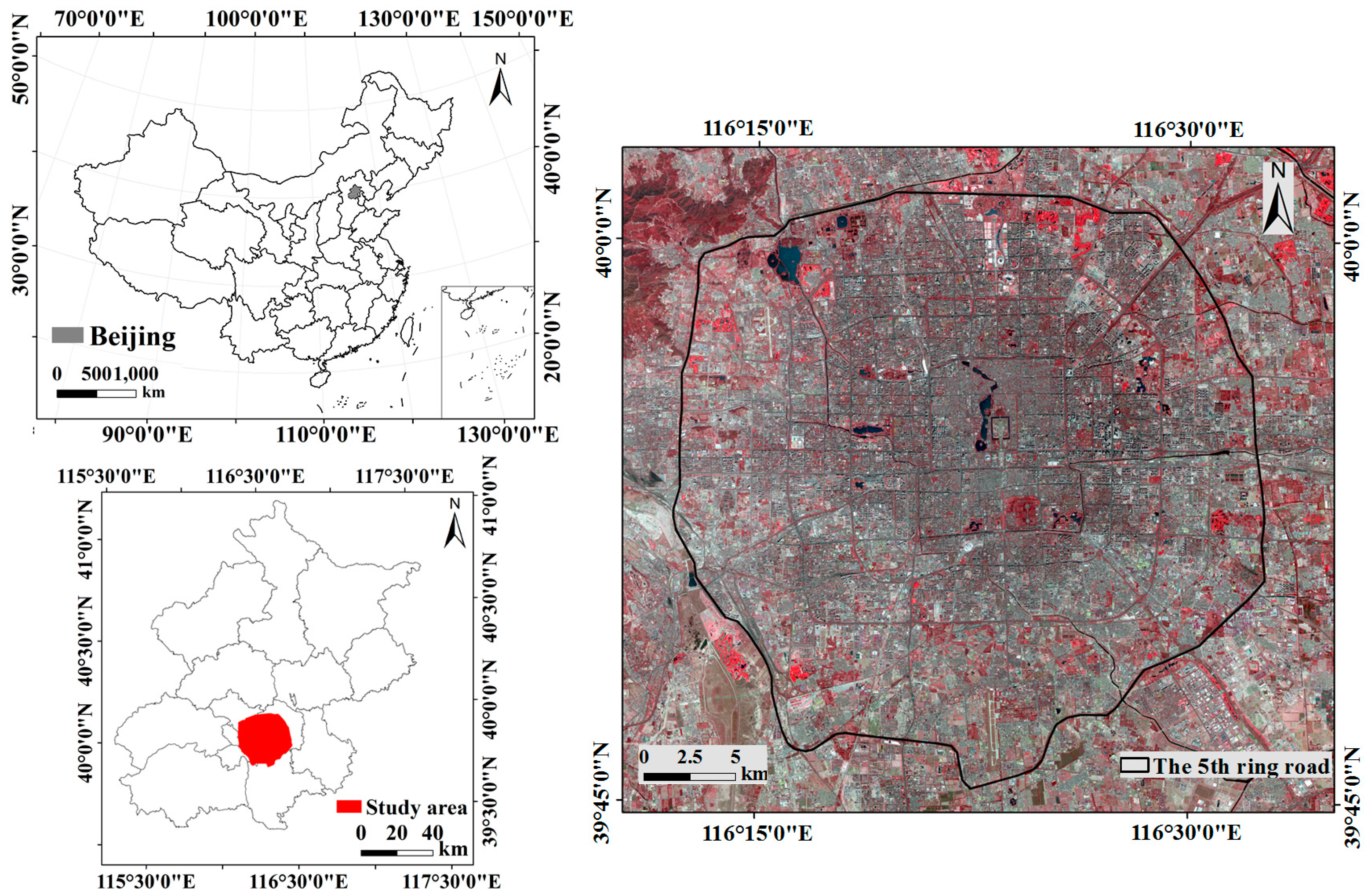
Our study focused on the area within the 5th ring road of Beijing, China (
Figure 1). Beijing is the capital of China, located in the northwestern part of the North China Plain (39°28′–41°25′N, 115°25′–117°30′E). It has an area of approximately 16,800 km
2, and a total population of more than 22 million in 2016 [
29]. In recent decades, Beijing has experienced a rapid urban expansion, with large areas of natural and agricultural land being converted into built-up areas [
20,
30].
The study area within the 5th ring road of Beijing has a size of approximately 666 km
2 and a total population of 10 million [
29]. It is the most developed region in Beijing. The study area is mixed with many different types of land use, and residential land use is one of the dominant uses, accounting for 26.28% of the total area. With the outward expansion and within-city renewal and redevelopment, residential landscape within the study area is spatial heterogeneous and diverse.
2.2. Data
2.2.1. Mapping the Residential Neighborhood
We used the residential neighborhood as the unit analysis. The first step was to map the boundaries of the residential neighborhood in the study area. We did this by visual interpretation based on 1 m spatial resolution GeoEye imagery acquired in 2009, with the aid of zoning maps from Baidu
TM map data (
map.baidu.com) circa 2010. Information from the website of a real-estate sale company, Lianjia
TM (
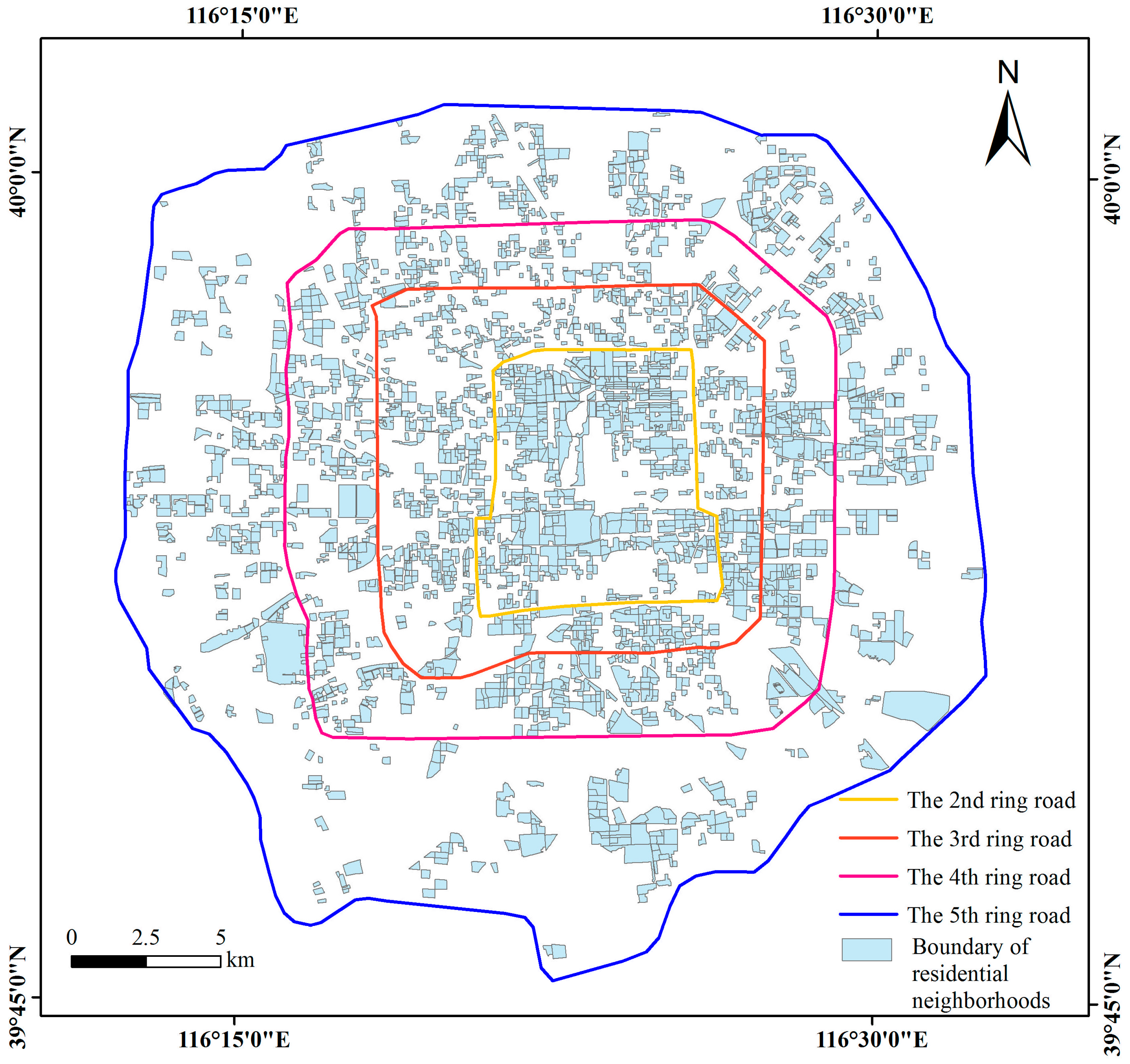
www.lianjia.com) was also used during the process of mapping. In addition, the built years (i.e., housing age) of these neighborhoods were obtained from this website. For the rebuilt neighborhood, the built time is the year in which it was rebuilt. In total, we mapped 2523 residential neighborhoods within the 5th ring road in Beijing (
Figure 2). We classified the residential neighborhoods into 5 types based on the built years, which were 1949–1978, 1978–1987, 1988–1997, 1998–2004, and 2005–2009 (
Table 1). We did this based on the years when major housing policies were implemented in China.
2.2.2. Building Footprint and Height Data
We obtained the data of building footprints and their heights of the residential neighborhoods from Baidu
TM map data circa 2010. By referring to the 1 m spatial resolution GeoEye imagery, we found most of the buildings were mapped in the building footprint dataset. The very few missing buildings were digitized by referring to the GeoEye imagery. We calculated the building density for each neighborhood (
Table 2).
The dataset also included the number of floors for each building. However, such information was missing for a considerable amount of buildings. We used the street view of Baidu
TM map to obtain the number of floors for those buildings. We further calculated the building height by multiplying the number of floors by 3 m, which is defined as the typical height of one floor by the Residential Building Code [
31].
In addition, we classified the residential neighborhoods into four categories based on the number of floors of the buildings within the neighborhoods (
Table 3), following the Chinese building classification in the Code for Design of Civil Buildings [
32].
2.2.3. High Resolution Land Cover Data
High spatial resolution land cover data were also used in this study to investigate the land cover and changes within each residential neighborhood. We used Advanced Land Observation Satellite (ALOS) imagery for land cover classification. The ALOS imagery has a panchromatic band with resolution of 2.5 m and four multispectral bands with resolution of 10 m. The imagery was acquired in 22 October 2009. We pan-sharpened the multispectral bands with the panchromatic band, resulting in multispectral bands with a spatial resolution of 2.5 m.
We used an object-based approach for land cover classification. An object-based approach first segments the imagery into objects, on which classification is then conducted [
23,
33]. An object-based approach provides a more effective and efficient means for high spatial resolution imagery classification, as it can not only use the spectral information, but also texture, context, and spatial relation [
23,
33]. We identified four land cover classes in this study, including vegetation, impervious surface (including buildings), water and bare soil. The overall accuracy of classification was 94.14%, with a Kappa statistic of 0.92. We calculated the vegetation coverage for each residential neighborhood (
Table 2).
2.3. Statistical Analysis
Our statistical analysis focused on how the 2-dimensional metrics (i.e., building density and vegetation coverage) and 3-dimensional metric (i.e., building height) changed through time. We first used Kruskal–Wallis one-way analysis of variance (ANOVA) to test whether the residential neighborhoods built in the 5 different periods had significant differences in proportional vegetation coverage, building density, and building height. We then used Pearson correlation analysis to examine the relationships between the built year of residential neighborhoods and the building density, proportional vegetation coverage, and building height.
3. Results
3.1. The Spatiotemporal Pattern of Residential Landscape in Beijing
3.1.1. Expansion of the Residential Landscape
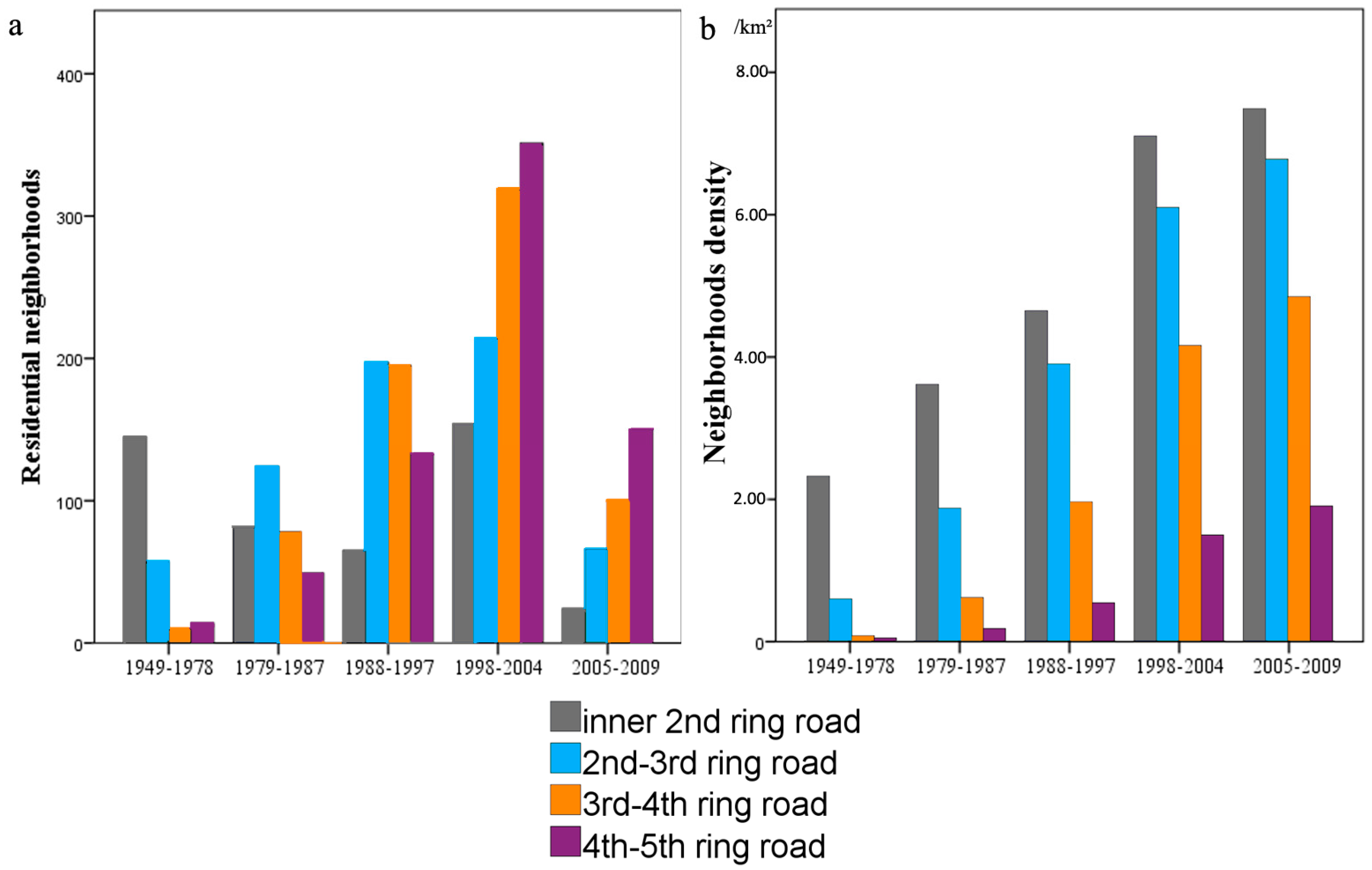
The expansion of the residential neighborhoods was dominated by outward growth, with much less within-city infilling development (
Figure 3 and
Figure 4). More than 60% of the residential neighborhoods built before 1978 were located in the urban core areas within the 2nd ring road. The residential neighborhoods built during the time period of 1979–1987 mostly occurred between the 2nd and 3rd ring road, with a percentage of 37.3%. From 1988–1997, newly built residential neighborhoods expanded outwards and were mainly located in areas between the 2nd and 3rd ring road and the 3rd ring and 4th ring road, with percentages of 33.4% and 33.1%, respectively. The residential neighborhoods expanded continuously outwards, with new neighborhoods mostly in the locations between the 4th and 5th ring road during the time period of 1998–2009. The proportion of newly built residential neighborhoods located between the 4th and 5th ring road was 33.8% in 1998–2004, and 44.1% in 2005–2009. While the development of the residential neighborhoods mainly tended to expand outwards, within-city infilling development increased through time, particularly in recent years. For example, more than 40% of the residential neighborhoods located in the area between the 2nd and 3rd ring road were built during 1998–2009 (
Figure 3 and
Figure 4a).
Although the region between the 3rd and 5th ring road had more residential neighborhoods, the region within the 3rd ring road had a higher neighborhood density (
Figure 3 and
Figure 4b). The region within the 2nd ring road had the highest density in all 5 periods, and the area between the 4th and 5th ring road always had a consistently lower neighborhood density than other regions. Neighborhood density in Beijing had a rapid growth during the period of 1998–2004 and then slowed during 2005–2009.
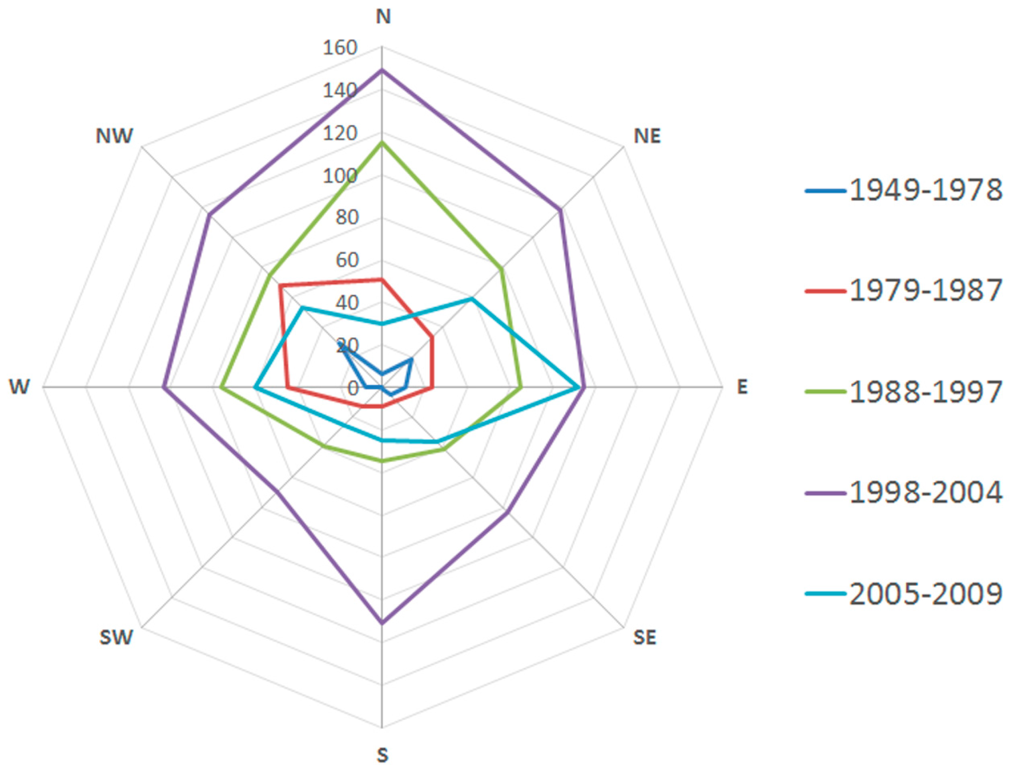
The spatial distribution of the residential neighborhoods is heterogeneous and varied by time. The majority of the residential neighborhoods is located in the northern and eastern region of Beijing, with much less in the southern part (
Figure 5). The residential neighborhoods built before 1979 are mainly located in the urban center area (64.2%). Approximately 41% of the residential neighborhoods built during 1979–1987 are located in the western and northwestern part of Beijing. The residential neighborhoods expanded towards the northern (21.9%) and northeastern (15.0%) part during 1988–1997. During 1998–2004, the residential neighborhoods expanded notably in all directions. An increased number of residential neighborhoods was built in the southern part (13.6%), but still less than that in the northern (17.7%) and northeastern (14.0%) regions of Beijing. Most of the residential neighborhoods built during 2005–2009 are located in the eastern region of Beijing (24.2%). Overall, the development of the residential neighborhoods in Beijing shifted from west to north in a clockwise direction (
Figure 5). This dramatic increase in the residential neighborhoods in all directions might be related to the housing policies in this time period, during which another round of housing institution reform was implemented (
Table 1).
The growth rate varied greatly through time, with a continuous increase from 1949–2004 and then a decrease from 2005–2009 (
Table 4). The total area of the residential neighborhoods that developed during the time period of 1949–1978 was 18.09 km
2, with the lowest annual growth rate (0.6 km
2/year). However, the mean size of the residential neighborhoods built during this time period was the largest (8 ha). The residential neighborhoods started to expand rapidly from 1979. The total area of the residential neighborhoods increased by 19.81 km
2 in 1979–1987, 35.42 km
2 in 1988–1997, and 66.82 km
2 in 1998–2004, with an annual growth rate of 2.2 km
2, 3.54 km
2, and 9.55 km
2, respectively. The size of the residential neighborhoods became smaller (6 ha) and was similar in these three time periods. The growth rate slowed to 5.02 km
2/year from 2005–2009, resulting in a total area of 25.11 km
2 in newly developed residential areas.
3.1.2. Vertical Structure of the Residential Landscape
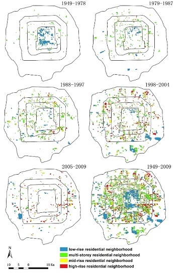
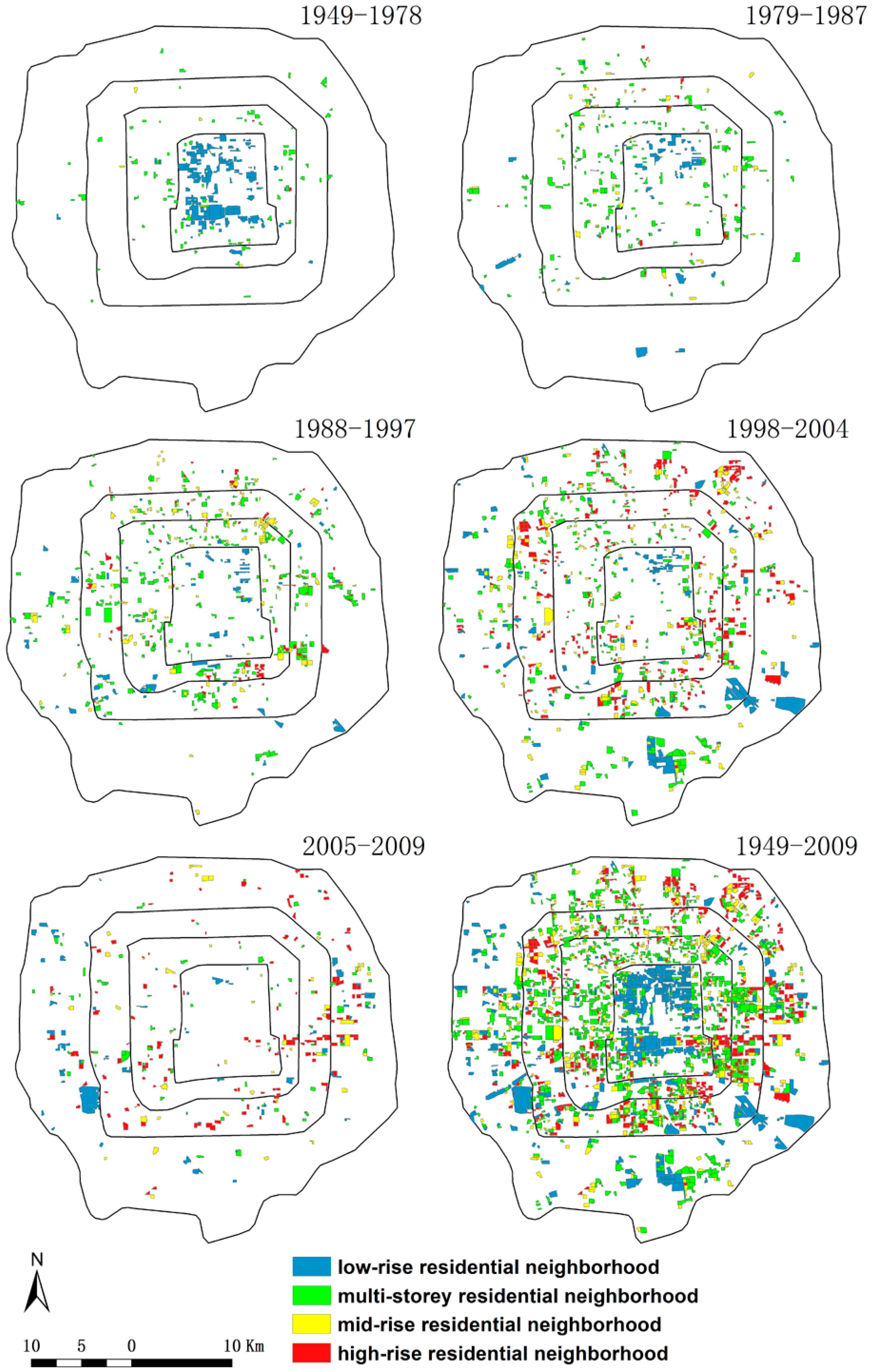
The vertical structure of the residential neighborhoods changed greatly through time from 1949–2009 (
Figure 3 and
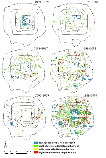
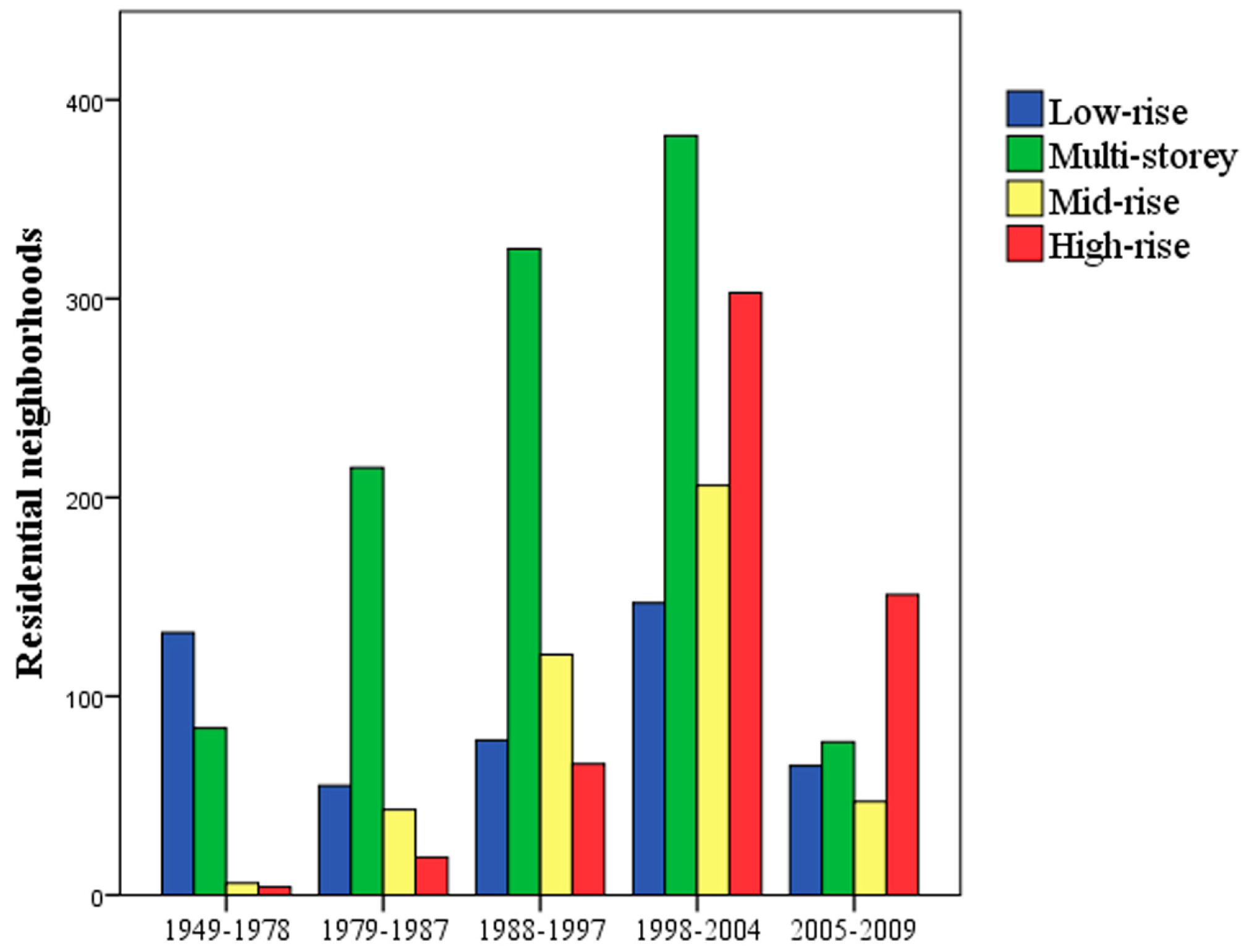
Figure 6). Most of the residential neighborhoods built before 1979 were low-rise residential neighborhoods with buildings of no more than 3 floors. There were few residential neighborhoods having buildings with more than 6 floors. The percentage of mid-rise and high-rise residential neighborhoods was only 4.5% during that time period. The residential neighborhoods built from 1979–2004 were dominated by buildings with 4–6 floors, particularly in the early years. For example, 64.8% of the buildings had 4–6 floors. Meanwhile, the proportion of high-rise buildings continued to increase, from only 5.7% in 1979–1988 to 11.2% in 1989–1997, and 29.2% in 1998–2004. During 2005–2009, high-rise apartments became the dominant building type in the residential neighborhoods, accounting for 44.4%. As discussed above, the residential neighborhoods mostly expanded outwards. Consequently, the vertical structure of the residential landscape was gradually built into a “low in the center, high at the edge” form. That is, the low-rise residential neighborhoods with a relatively long history within the 2nd ring road were surrounded by medium- and high-rise residential neighborhoods distributed between the 3rd and 5th ring road in Beijing (
Figure 3).
3.2. Changes within Residential Neighborhoods through Time
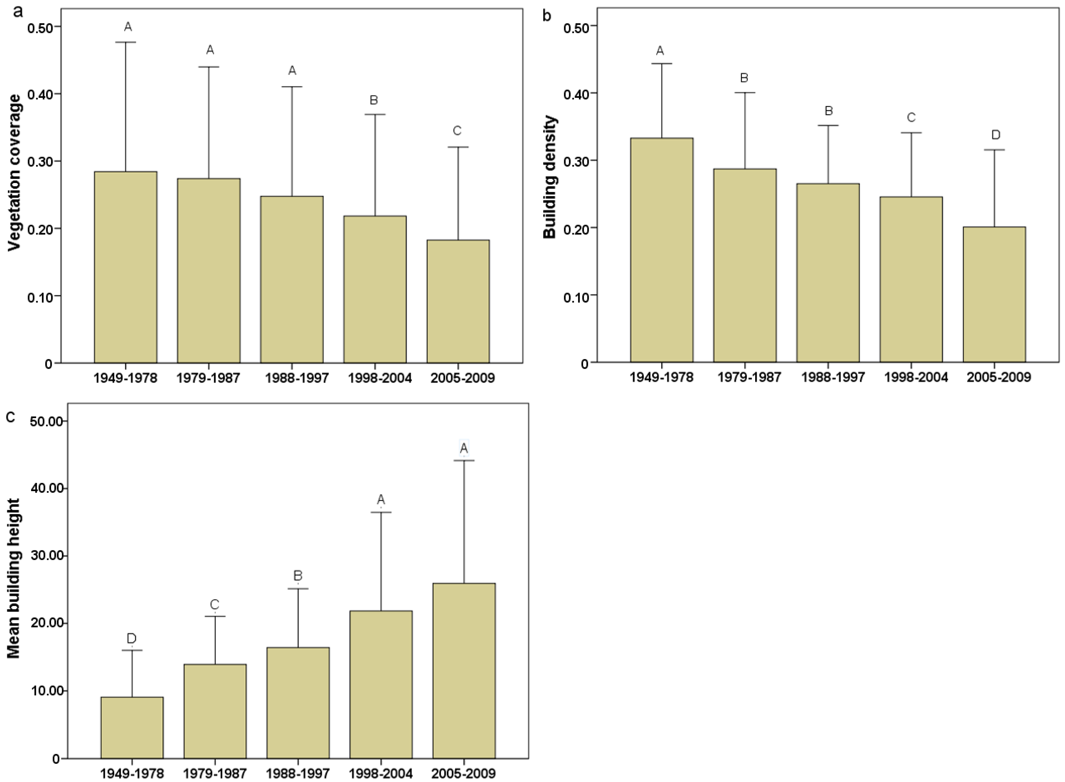
We found the residential neighborhoods built in different time periods had significant differences in vegetation coverage, building density, and building height (
Figure 7). The highest proportional vegetation coverage occurred in the residential neighborhoods built in 1979–1978 (0.28), while the lowest coverage occurred in 2005–2009 (0.20). The residential neighborhoods built in 1949–1978 had the highest building density (0.33) and the lowest average building height (9.07 m), whereas those built in 2004–2009 had the lowest building density (0.2) but the greatest height (25.93 m).
The Pearson correlation analysis results showed that vegetation coverage, building density and building height were all significantly correlated with the built year of residential neighborhoods (
Table 5). Building height had a significantly positive relationship with built year, while building density and vegetation coverage had significantly negative relationships (
Table 5). Further correlation analyses were conducted to investigate the relationship between vegetation coverage, building density and building height (
Table 5 and
Table 6). The results showed that there was a significantly negative correlation between building density and vegetation coverage, while building height had a significantly negative relationship with both of these variables from 1949–2009. In the five time periods, the vegetation coverage was negatively correlated with building density, and building height had a significantly negative relationship with building density, but building height had no significant correlation with vegetation coverage in all five time periods.
4. Discussion
Our results on the changes in the building height of the residential landscapes underscore the importance of considering the vertical dimension in spatial pattern analysis. The commonly used two-dimensional analysis may miss important changes in the residential landscapes. For example, there was no significant difference in building density and vegetation coverage between the residential neighborhoods built in the two time periods of 1979–1987 and 1988–1997 (
Figure 7a,b). However, the average building height of residential neighborhoods greatly increased from 13.9 m in 1979–1987 to 16.4 m in 1988–1997 (
Figure 7c). Previous studies have also demonstrated that the inclusion of the vertical dimension can provide better understanding of changes in landscapes (e.g., [
34,
35]).
Our results showed that building height varied greatly in the residential neighborhoods built in different years. The residential neighborhoods built in more recent years tended to have more tall buildings and thus greater average building height. These high-rise residential apartments were built to meet the need of accelerated population growth in Beijing and to improve the land use efficiency [
36,
37]. The changes in the height of the residential neighborhoods and their spatial distribution may have great social-ecological implications. On the one hand, extending “urban growth” to the vertical dimension, that is, building high-rise apartments, can greatly improve the land use efficiency, and therefore reduce the adverse impacts of urban expansion on replacing natural landscapes or agricultural lands. The increase in open space and greenspace in a residential neighborhood can also provide a variety of social and ecological benefits to its residents [
38,
39,
40,
41]. In addition, the living environment of residential neighborhoods can benefit from building high-rise apartments in some aspects [
42]. For example, the residential neighborhoods with greater average building height tend to have lower land surface temperature [
43,
44,
45]. This is likely because the residential neighborhoods with higher buildings tend to have lower building density, and higher proportional greenspace coverage (
Table 5 and
Table 6). Additionally, high-rise buildings can provide large shaded areas that also can effectively reduce the surface and air temperature [
44,
46,
47].
On the other hand, the spatial distribution of the residential neighborhoods with different building height may have some adverse social and ecological impacts. In Beijing, the downtown area is mostly dominated by the residential neighborhoods with relative low buildings, which is surrounded by high-rise apartments located from the 3rd ring road to the 5th ring road. This forms a “low-high” pattern from the central area to the edge (
Figure 3). Taking the thermal environment as an example again, these clusters of neighborhoods with high-rise buildings in the outer-rings may block urban ventilation [
48,
49] and therefore aggravate the urban heat island effects, as well as prevent the diffusion of air pollutants in the urban central areas [
24,
50,
51]. The social and ecological impacts of the vertical structure warrant further research.
Recent advances in Light Detecting and Ranging (LiDAR) and unmanned aerial vehicle technology greatly increase the availability of vertical dimensional data in an affordable way [
52,
53,
54,
55]. These advances will greatly facilitate the quantitative analysis of the vertical structure of the urban landscapes and their social and ecological impacts. Such analysis would be highly desirable, not only for urban ecologists to better understand the structure of the urban landscape, but also for urban planners and designers to better manage the urban landscape.
5. Conclusions
Quantifying the vertical structure of the urban landscape and its change is important to understand its social and ecological impacts. Our study focuses on the residential landscape to investigate how the vertical dimension of the urban landscape (i.e., building height) changes through time and how such change is related to changes in the horizontal dimension of the landscape. We found that (1) in different time periods, the spatial distribution of newly built residential neighborhoods is different. Overall, the expansion mode of the residential neighborhoods within the 5th ring road in Beijing during 1949–2009 was dominated by outward growth, with much less within-city infilling. The growth rate varied greatly through time, first increasing from 1949–2004 and then decreasing from 2005–2009. The neighborhood density is higher in center area and lower in urban edges. The expansion direction of newly built residential neighborhoods shifted from west to north in a clockwise direction. (2) The residential neighborhoods also developed in the vertical space, which formed a “low-high” pattern from the urban central area to the urban edges within the 5th ring road in Beijing. (3) The landscape pattern of the residential neighborhoods in different time periods is significantly different. The residential neighborhoods built in more recent years tend to have taller buildings, lower building density and lower vegetation coverage than other periods. There was a significantly negative correlation between building density and vegetation coverage, while building height had a significantly negative relationship with both of these variables from 1949–2009.
Our study reveals the distribution of the residential neighborhoods and the change of the residential landscape within the 5th ring road in Beijing during 1949–2009. The study aims to strengthen the understanding of residential area change and to provide a methodological basis for urban planning and policy making. This paper did not involve the study of the driving force underlying the change in residential neighborhood landscape patterns, which has great significance for urban planning. It could be studied in further research.
Acknowledgments
This research was funded by the National Natural Science Foundation of China (Grant No. 41422104 and 41590841), the project “Developing key technologies for establishing ecological security patterns at the Beijing-Tianjin-Hebei urban megaregion” of the National key research and development program (2016YFC0503004), and the Key Research Program of Frontier Sciences, CAS (QYZDB-SSW-DQC034).
Author Contributions
Weiqi Zhou designed this research. Zhong Zheng, Weiqi Zhou, Jia Wang, Xiaofang Hu and Yuguo Qian analyzed the data. Zhong Zheng and Weiqi Zhou wrote the paper.
Conflicts of Interest
The authors declare no conflict of interest.
References
- Wu, J. Urban ecology and sustainability: The state-of-the-science and future directions. Landsc. Urban Plan. 2014, 125, 209–221. [Google Scholar] [CrossRef]
- Zhou, W.; Pickett, S.T.A.; Cadenasso, M.L. Shifting concepts of urban spatial heterogeneity and their implications for sustainability. Landsc. Ecol. 2017, 32, 15–30. [Google Scholar] [CrossRef]
- Pickett, S.T.; Cadenasso, M.L.; Grove, J.M.; Boone, C.G.; Groffman, P.M.; Irwin, E.; Kaushal, S.S.; Marshall, V.; Mcgrath, B.P.; Nilon, C.H. Urban ecological systems: Scientific foundations and a decade of progress. J. Environ. Manag. 2011, 92, 331–362. [Google Scholar] [CrossRef] [PubMed]
- Zhou, W.; Huang, G.; Pickett, S.T.A.; Cadenasso, M.L. 90 years of forest cover change in an urbanizing watershed: Spatial and temporal dynamics. Landsc. Ecol. 2011, 26, 645–659. [Google Scholar] [CrossRef]
- Grimm, N.B.; Foster, D.; Groffman, P.; Grove, J.M.; Hopkinson, C.S.; Nadelhoffer, K.J.; Pataki, D.E.; Peters, D.P.C. The changing landscape: Ecosystem responses to urbanization and pollution across climatic and societal gradients. Front. Ecol. Environ. 2008, 6, 264–272. [Google Scholar] [CrossRef]
- Seto, K.C.; Güneralp, B.; Hutyra, L. Global forecasts of urban expansion to 2030 and direct impacts on biodiversity and carbon pools. Proc. Natl. Acad. Sci. USA 2012, 109, 16083–16088. [Google Scholar] [CrossRef] [PubMed]
- Grimm, N.B.; Faeth, S.H.; Golubiewski, N.E.; Redman, C.L.; Wu, J.; Bai, X.; Briggs, J.M. Global change and the ecology of cities. Science 2008, 319, 756–760. [Google Scholar] [CrossRef] [PubMed]
- Han, L.; Zhou, W.; Li, W. Increasing impact of urban fine particles (PM2.5) on areas surrounding Chinese cities. Sci. Rep. 2015, 5. [Google Scholar] [CrossRef] [PubMed]
- Huang, G. PM2.5 opened a door to public participation addressing environmental challenges in China. Environ. Pollut. 2015, 197, 313–315. [Google Scholar] [CrossRef] [PubMed]
- Peng, J.; Chen, S.; Lü, H.; Liu, Y.; Wu, J. Spatiotemporal patterns of remotely sensed PM2.5 concentration in China from 1999 to 2011. Remote Sens. Environ. 2016, 174, 109–121. [Google Scholar] [CrossRef]
- Zhou, W.; Wang, J.; Cadenasso, M.L. Remote Sensing of Environment Effects of the spatial con fi guration of trees on urban heat mitigation: A comparative study. Remote Sens. Environ. 2017, 195, 1–12. [Google Scholar] [CrossRef]
- Huang, G.; Cadenasso, M.L. People, landscape, and urban heat island: Dynamics among neighborhood social conditions, land cover and surface temperatures. Landsc. Ecol. 2016, 31, 2507–2515. [Google Scholar] [CrossRef]
- Zhou, W.; Qian, Y.; Li, X.; Li, W.; Han, L. Relationships between land cover and the surface urban heat island: Seasonal variability and effects of spatial and thematic resolution of land cover data on predicting land surface temperatures. Landsc. Ecol. 2014, 29, 153–167. [Google Scholar] [CrossRef]
- Miller, R.B.; Small, C. Cities from space: Potential applications of remote sensing in urban environmental research and policy. Environ. Sci. Policy 2003, 6, 129–137. [Google Scholar] [CrossRef]
- Bhatta, B.; Saraswati, S.; Bandyopadhyay, D. Urban sprawl measurement from remote sensing data. Appl. Geogr. 2010, 30, 731–740. [Google Scholar] [CrossRef]
- Mertes, C.M.; Schneider, A.; Sulla-Menashe, D.; Tatem, A.J.; Tan, B. Detecting change in urban areas at continental scales with modis data. Remote Sens. Environ. 2015, 158, 331–347. [Google Scholar] [CrossRef]
- Tan, K.C.; Lim, H.S.; Matjafri, M.Z.; Abdullah, K. Landsat data to evaluate urban expansion and determine land use/land cover changes in Penang Island, Malaysia. Environ. Earth Sci. 2010, 60, 1509–1521. [Google Scholar] [CrossRef]
- Lu, D.; Li, G.; Kuang, W.; Moran, E. Methods to extract impervious surface areas from satellite images. Int. J. Digit. Earth 2014, 7, 93–112. [Google Scholar] [CrossRef]
- Stow, D.A.; Chen, D.M. Sensitivity of multitemporal noaa avhrr data of an urbanizing region to land-use/land-cover changes and misregistration. Remote Sens. Environ. 2002, 80, 297–307. [Google Scholar] [CrossRef]
- Wei, S.; Pijanowski, B.C.; Tayyebi, A. Urban expansion and its consumption of high-quality farmland in Beijing, China. Ecol. Indic. 2015, 54, 60–70. [Google Scholar]
- Qian, Y.; Zhou, W.; Li, W.; Han, L. Understanding the dynamic of greenspace in the urbanized area of Beijing based on high resolution satellite images. Urban For. Urban Green. 2015, 14, 39–47. [Google Scholar] [CrossRef]
- Qian, Y.; Zhou, W.; Yu, W.; Pickett, S.T.A. Quantifying spatiotemporal pattern of urban greenspace: New insights from high resolution data. Landsc. Ecol. 2015, 30, 1165–1173. [Google Scholar] [CrossRef]
- Zhou, W.; Troy, A.; Grove, M. Object-based land cover classification and change analysis in the baltimore metropolitan area using multitemporal high resolution remote sensing data. Sensors 2008, 8, 1613–1636. [Google Scholar] [CrossRef] [PubMed]
- Edussuriya, P.; Chan, A.; Ye, A. Urban morphology and air quality in dense residential environments in hong kong. Part I: District-level analysis. Atmos. Environ. 2011, 45, 4789–4803. [Google Scholar] [CrossRef]
- Lin, J.; Huang, B.; Chen, M.; Huang, Z. Modeling urban vertical growth using cellular automata—Guangzhou as a case study. Appl. Geogr. 2014, 53, 172–186. [Google Scholar] [CrossRef]
- Unger, J. Modelling of the annual mean maximum urban heat island using 2d and 3d surface parameters. Clim. Res. 2006, 30, 215–226. [Google Scholar] [CrossRef]
- Broitman, D.; Koomen, E. Residential density change: Densification and urban expansion. Comput. Environ. Urban Syst. 2015, 54, 32–46. [Google Scholar] [CrossRef]
- An, L.; Brown, D.G.; Nassauer, J.I.; Low, B. Variations in development of exurban residential landscapes: Timing, location, and driving forces. J. Land Use Sci. 2011, 6, 13–32. [Google Scholar] [CrossRef]
- Beijing Municipal Statistical Bureau. Beijing Statistical Yearbook 2016; China Statistics Press: Beijing, China, 2016.
- Li, X.; Zhou, W.; Ouyang, Z. Forty years of urban expansion in Beijing: What is the relative importance ofphysical, socioeconomic, and neighborhood factors? Appl. Geogr. 2013, 38, 1–10. [Google Scholar] [CrossRef]
- Ministry of Construction of the People’s Republic of China. Residential Building Code; China Architecture & Building Press: Beijing, China, 2005.
- Ministry of Construction of the People’s Republic of China. Code for Design of Civil Buildings; China Architecture & Building Press: Beijing, China, 2005.
- Qian, Y.; Zhou, W.; Yan, J.; Li, W.; Han, L. Comparing machine learning classifiers for object-based land cover classification using very high resolution imagery. Remote Sens. 2014, 7, 153–168. [Google Scholar] [CrossRef]
- Chen, Z.; Xu, B.; Devereux, B. Urban landscape pattern analysis based on 3d landscape models. Appl. Geogr. 2014, 55, 82–91. [Google Scholar] [CrossRef]
- Koomen, E.; Rietveld, P.; Bacao, F. The third dimension in urban geography: The urban-volume approach. Environ. Plan. B Plan. Des. 2009, 36, 1008–1025. [Google Scholar] [CrossRef]
- Ding, C. Building height restrictions,land development and economic costs. Land Use Policy 2013, 30, 485–495. [Google Scholar] [CrossRef]
- Zhou, P.; Liu, Y.; Chen, Y.; Zeng, C.; Wang, Z. Prediction of the spatial distribution of high-rise residential buildings by the use of a geographic field based autologistic regression model. J. Hous. Built Environ. 2015, 30, 487–508. [Google Scholar] [CrossRef]
- Esbah, H.; Cook, E.A.; Ewan, J. Effects of increasing urbanization on the ecological integrity of open space preserves. Environ. Manag. 2009, 43, 846–862. [Google Scholar] [CrossRef] [PubMed]
- Wu, J.J.; Plantinga, A.J. The influence of public open space on urban spatial structure. J. Environ. Econ. Manag. 2003, 46, 288–309. [Google Scholar] [CrossRef]
- Ying, Z.; Ning, L.D.; Xin, L. Relationship between built environment, physical activity, adiposity, and health in adults aged 46–80 in Shanghai, China. J. Phys. Act. Health 2015, 12, 569. [Google Scholar] [CrossRef] [PubMed]
- Beyer, K.M.; Kaltenbach, A.; Szabo, A.; Bogar, S.; Nieto, F.J.; Malecki, K.M. Exposure to neighborhood green space and mental health: Evidence from the survey of the health of wisconsin. Int. J. Environ. Res. Public Health 2014, 11, 3453–3472. [Google Scholar] [CrossRef] [PubMed]
- Forman, R.T.T. Urban Ecology: Science of Cities; Cambridge University Press: Cambridge, UK, 2014. [Google Scholar]
- Li, J.; Song, C.; Cao, L.; Zhu, F.; Meng, X.; Wu, J. Impacts of landscape structure on surface urban heat islands: A case study of Shanghai, China. Remote Sens. Environ. 2011, 115, 3249–3263. [Google Scholar] [CrossRef]
- Lindberg, F.; Grimmond, C.S.B. The influence of vegetation and building morphology on shadow patterns and mean radiant temperatures in urban areas: Model development and evaluation. Theor. Appl. Climatol. 2011, 105, 311–323. [Google Scholar] [CrossRef]
- Yang, X.; Li, Y. The impact of building density and building height heterogeneity on average urban albedo and street surface temperature. Build. Environ. 2015, 90, 146–156. [Google Scholar] [CrossRef]
- Berardi, U.; Wang, Y. The effect of a denser city over the urban microclimate: The case of Toronto. Sustainability 2016, 8, 22. [Google Scholar] [CrossRef]
- Ali, J.M.; Marsh, S.H.; Smith, M.J. Modelling the spatiotemporal change of canopy urban heat islands. Build. Environ. 2016, 107, 64–78. [Google Scholar] [CrossRef]
- Gál, T.; Unger, J. Detection of ventilation paths using high-resolution roughness parameter mapping in a large urban area. Build. Environ. 2009, 44, 198–206. [Google Scholar] [CrossRef]
- Man, S.W.; Nichol, J.E.; To, P.H.; Wang, J. A simple method for designation of urban ventilation corridors and its application to urban heat island analysis. Build. Environ. 2010, 45, 1880–1889. [Google Scholar]
- Yuan, S.; Lau, K.L.; Ng, E. Developing street-level pm2.5 and pm10 land use regression models in high-density Hong Kong with urban morphological factors. Environ. Sci. Technol. 2016, 50, 8178–8187. [Google Scholar]
- Buccolieri, R.; Sandberg, M.; Sabatino, S.D. An application of ventilation efficiency concepts to the analysis of building density effects on urban flow and pollutant concentration. Int. J. Environ. Pollut. 2011, 47, 248–256. [Google Scholar] [CrossRef]
- Zhang, W.; Wang, H.; Chen, Y.; Yan, K.; Chen, M. 3d building roof modeling by optimizing primitive’s parameters using constraints from lidar data and aerial imagery. Remote Sens. 2014, 6, 8107–8133. [Google Scholar] [CrossRef]
- Zhou, W. An object-based approach for urban land cover classification: Integrating lidar height and intensity data. IEEE Geosci. Remote Sens. Lett. 2013, 10, 928–931. [Google Scholar] [CrossRef]
- D’Oleireoltmanns, S.; Marzolff, I.; Peter, K.D.; Ries, J.B. Unmanned aerial vehicle (uav) for monitoring soil erosion in morocco. Remote Sens. 2012, 4, 3390–3416. [Google Scholar] [CrossRef]
- Wu, B.; Yu, B.; Wu, Q.; Yao, S.; Zhao, F.; Mao, W.; Wu, J. A graph-based approach for 3d building model reconstruction from airborne lidar point clouds. Remote Sens. 2017, 9, 92. [Google Scholar] [CrossRef]
Figure 1.
Study Area: the region within the fifth ring road of Beijing, China.
Figure 1.
Study Area: the region within the fifth ring road of Beijing, China.
Figure 2.
Spatial distribution of the residential neighborhoods within the 5th ring road of Beijing.
Figure 2.
Spatial distribution of the residential neighborhoods within the 5th ring road of Beijing.
Figure 3.
Spatial distribution of the residential neighborhoods within the 5th ring road of Beijing in different time periods.
Figure 3.
Spatial distribution of the residential neighborhoods within the 5th ring road of Beijing in different time periods.
Figure 4.
Quantity changes of the residential neighborhoods in regions within the 5th ring road of Beijing in different time periods: (a) Number of newly built residential neighborhoods; (b) Variation of neighborhood density, where neighborhood density is the number of residential neighborhoods per km2.
Figure 5.
Distribution of the residential neighborhoods within the 5th ring road of Beijing in different directions.
Figure 5.
Distribution of the residential neighborhoods within the 5th ring road of Beijing in different directions.
Figure 6.
Number of different residential neighborhood types within the 5th ring road of Beijing in different time periods.
Figure 6.
Number of different residential neighborhood types within the 5th ring road of Beijing in different time periods.
Figure 7.
Results of one-way ANOVA on (a) vegetation coverage, (b) building density and (c) building height among different time periods. Superscripted letters indicate a significant difference among different time periods (p < 0.05). Different letters indicate significant differences, and the same letters indicate no significant difference.
Table 1.
The five periods when major housing policies were implemented in China.
Table 1.
The five periods when major housing policies were implemented in China.
| Periods | Year | Description |
|---|
| 1 | 1949–1978 | Before the reform and opening-up policy, with only public owned houses provided for residents. |
| 2 | 1979–1987 | The implementation of the reform and opening-up policy, with the appearance of some private residential buildings. |
| 3 | 1988–1997 | The early years of the housing institution reform and the start of real estate industry; during this time period, the availability of public owned houses decreased. |
| 4 | 1998–2004 | Starting another round of housing institution reform, with dramatic increasing of private residential buildings. The government stopped housing allocation. |
| 5 | 2005–2009 | Period in which the government controlled the real estate market to rein in property prices. |
Table 2.
Variables of characteristics of the residential neighborhood.
Table 2.
Variables of characteristics of the residential neighborhood.
| | Parameters | Unit | Formulas |
|---|
| Features | Built year | year | |
| | Area of residential neighborhood (S) | m2 | |
| | Number of annual built neighborhoods | - | |
| 2D Landscape metrics | Building density (BD) | - | |
| | Vegetation coverage (VC) | - | |
| 3D Landscape metric | Mean building height () | m | |
Table 3.
Classification of the residential neighborhoods in terms of building height.
Table 3.
Classification of the residential neighborhoods in terms of building height.
| Types | Storey | Number (Percentage) | Area (ha) (Percentage) |
|---|
| Low-rise residential neighborhood | 1–3 | 474 (18.8%) | 87.86 (40.2%) |
| Multi-storey residential neighborhood | 4–6 | 1083 (42.9%) | 75.95 (34.7%) |
| Mid-rise residential neighborhood | 7–9 | 423 (16.8%) | 23.33 (10.6%) |
| High-rise residential neighborhood | >9 | 543 (21.5%) | 31.79 (14.5%) |
Table 4.
Expansion of the residential neighborhoods in different time periods.
Table 4.
Expansion of the residential neighborhoods in different time periods.
| Classification | Built Year | Total Area of Newly Built Residential Neighborhoods (km2) | Annual Increasing Rate of Residential Neighborhoods (km2/year) | Mean Area of Residential Neighborhoods (ha) |
|---|
| 1 | 1949–1978 | 18.09 | 0.6 | 8.0 |
| 2 | 1979–1987 | 19.81 | 2.2 | 6.0 |
| 3 | 1988–1997 | 35.42 | 3.54 | 6.0 |
| 4 | 1998–2004 | 66.82 | 9.55 | 6.4 |
| 5 | 2005–2009 | 25.11 | 5.02 | 7.4 |
Table 5.
Pearson correlation coefficients between built year of residential neighborhood and building height, building density, and vegetation coverage.
Table 5.
Pearson correlation coefficients between built year of residential neighborhood and building height, building density, and vegetation coverage.
| | Built Year | | BD | VC |
|---|
| Built year | 1 | 0.347 ** | −0.322 ** | −0.158 ** |
| | 1 | −0.317 ** | −0.095 ** |
| BD | | | 1 | −0.135 ** |
| VC | | | | 1 |
Table 6.
Pearson correlation coefficients between building height, building density and vegetation coverage in the five time periods.
Table 6.
Pearson correlation coefficients between building height, building density and vegetation coverage in the five time periods.
| | | | BD | VC |
|---|
| 1949–1978 | | 1 | −0.377 ** | 0.009 |
| BD | | 1 | −0.237 ** |
| VC | | | 1 |
| 1979–1987 | | 1 | −0.387 ** | −0.072 |
| BD | | 1 | −0.132 * |
| VC | | | 1 |
| 1988–1997 | | 1 | −0.288 ** | 0.072 |
| BD | | 1 | −0.231 ** |
| VC | | | 1 |
| 1998–2004 | | 1 | −0.237 ** | −0.05 |
| BD | | 1 | −0.245 ** |
| VC | | | 1 |
| 2005–2009 | | 1 | −0.159 ** | −0.088 |
| BD | | 1 | −0.139 * |
| VC | | | 1 |
© 2017 by the authors. Licensee MDPI, Basel, Switzerland. This article is an open access article distributed under the terms and conditions of the Creative Commons Attribution (CC BY) license (http://creativecommons.org/licenses/by/4.0/).


